Chaos Removal in the $R+qR^{2}$ gravity: the Mixmaster model

Abstract

We study the asymptotic dynamics of the Mixmaster Universe, near the cosmological singularity, considering $f(R)$ gravity up to a quadratic corrections in the Ricci scalar $R$. The analysis is performed in the scalar-tensor framework and adopting Misner-Chitré-like variables to describe the Mixmaster Universe, whose dynamics resembles asymptotically a billiard-ball in a given domain of the half-Poincaré space. The form of the potential well depends on the spatial curvature of the model and on the particular form of the self-interacting scalar field potential. We demonstrate that the potential walls determine an open domain in the configuration region, allowing the point-Universe to reach the absolute of the considered Lobachevsky space. In other words, we outline the existence of a stable final Kasner regime in the Mixmaster evolution, implying the chaos removal near the cosmological singularity. The relevance of the present issue relies both on the general nature of the considered dynamics, allowing its direct extension to the BKL conjecture too, as well as the possibility to regard the considered modified theory of gravity as the first correction to the Einstein-Hilbert action as a Taylor expansion of a generic function $f(R)$ (as soon as a cut-off on the space-time curvature takes place).

Introduction

The chaotic dynamics of the Mixmaster Universe BKLref1 ,mixmastermisner ,misner is a basic prototype of the local (sub-horizon) behaviour of the generic cosmological solution (the so-called BKL conjectureBKLref2 ). Investigating the stability of such a chaotic picture with respect to the presence of matter scalar field ,montanireview ,primordial and space-time dimensions numberhennaux1 ,hennaux2 ,del1 has seen a great effort over the last four decades and the most significant issue was the proof of the chaos removal when a massless scalar field is involved in the dynamics scalar field . Such a result is a consequence of the capability manifested by the scalar field kinetic energy of affecting the second (quadratic) Kasner condition, easily restated in the Hamiltonian picture, as shown in berger . This property of the massless scalar field acquires intriguing perspectives when $f(R)$ modified theory of gravity are considered capfirst ,capozzielloreview ,odintsovreview ,odintsov ,guo . In fact, these alternative formulation of the gravitational field dynamics can be represented by an equivalent scalar-tensor picture: the scalar degree of freedom associated to the form of the function $f$ is expressed via a self-interacting scalar field, coupled to the ordinary General Relativity bar1 ,bar2 ,bar3 ,del2 . When implementing this scalar-tensor scheme to the Mixmaster Universe dynamics, a natural question arise: the kinetic term of the scalar field removes the chaotic behaviour, but the presence of a potential term could restore it? Thus we can study, for specific modified theories of gravity, if the Mixmaster chaos survives or not, simply characterizing the corresponding scalar field potential. Here we analyse the modified gravity theory corresponding to a quadratic correction in the Ricci scalar to the ordinary Einstein-Hilbert Lagrangian, both because it is the simplest viable deviation from General Relativity (apart from a cosmological constant term), as well as the first correction emerging from a Taylor expansion of a $f(R)$ theory for very small values of the space-time Ricci scalar, i.e. for very law curvatures, like we observe today in the Solar Systemstaro1 . The quadratic term in the Ricci scalar provides an exponential-like potential term for the self-interacting scalar field, when a scalar-tensor reformulation of the model is considered. This case is particularly appropriate to the analysis we pursue of the Mixmaster dynamics in terms of the Misner-Chitré-like variables primordial ,montani-kirillov ,imponente-montani ,MCthesis . In fact, the kinetic term of the scalar field is on the same footing of the anisotropy term contribution and, for the considered Lagrangian, also the potential term is isomorphic to the spatial curvature of the model, i.e. the total potential term is constituted by equivalent exponential profile. In the asymptotic limit toward the initial singularity the total potential takes the form of four potential walls, whose morphology determines if the configuration domain is closed or not. Indeed, we demonstrate how the whole domain, available in principle, is a constant negative curvature space (half-Poincarè space). We first analyse the case of the Mixmaster Universe in the presence of a massless scalar field, demonstrating the open nature of its configuration space and the implied existence of a stable Kasner regime to the initial singularity. Then, we face a detailed study of the dynamics in the presence of the total potential and the still open structure of the configuration domain. Thus, we demonstrate the non-chaotic nature of the Mixmaster Universe behaviour, as it is described by the scalar-tensor version of the $R^{2}$-gravity.

$f(R)$ gravity

The $f(R)$ theories of gravity are a direct generalization of the Einstein-Hilbert Lagrangian consisting in a replacement of the Ricci Scalar $R$ by a general function $f(R)$capozzielloreview ,odintsovreview ,odintsov ,odintsov2 :

$$S=\frac{1}{16\pi}\int d^{4}x\sqrt{-g}f(R)$$ (1)

where $g$ is the determinant of the metric. The introduction of the additional degree of freedom, related to the presence of the $f(R)$ term, can be translated into a dynamics of a self-interacting scalar field coupled with the Einstein-Hilbert Action, the so-called Scalar-Tensor framework. In this approach, a new auxiliary field $\chi$ is introduced to get the following equivalent version of the action (1):

$$S=\frac{1}{16\pi}\int d^{4}x\sqrt{-g}[f(\chi)-f^{\prime}(\chi)(R-\chi)].$$ (2)

The variation of the action (2) with respect to $\chi$ provides $f^{\prime\prime}(\chi)(R-\chi)=0$, implying $\chi=R$ if $f^{\prime\prime}(\chi)\neq 0$. By a redefinition of the auxiliary field $\chi$ in the form $\varphi=f^{\prime}(\chi)$ the action becomes

$$S=\frac{1}{16\pi}\int d^{4}x\sqrt{-g}[\varphi R-\chi(\varphi)\varphi+f(\chi(\varphi))].$$ (3)

It is now possible to perform a conformal transformation on the metric $g_{\mu\nu}\rightarrow\tilde{g_{\mu\nu}}=\varphi g_{\mu\nu}$ and a scalar field redefinition $\varphi\equiv f^{\prime}(R)\rightarrow\phi=\sqrt{\frac{3}{16\pi}}\ln f^{\prime}(R)$ in order to obtain

$$S=\int d^{4}x\sqrt{-\tilde{g}}\left[\frac{\tilde{R}}{16\pi}-\frac{1}{2}\partial^{\alpha}\phi\partial_{\alpha}\phi-U(\phi)\right],$$ (4)

where the potential term $U(\phi)$ has the form:

$$U(\phi)=\frac{Rf^{\prime}(R)-f(R)}{16\pi(f^{\prime}(R))^{2}}.$$ (5)

For small values of the Ricci scalar, the first order correction to the Einstein-Hilbert Lagrangian, is represented by a quadratic correction, i.e.

$$f(R)=R+qR^{2}.$$ (6)

By this choice, the potential term (5) takes the form

$$U(\phi)=\frac{1}{64\pi q}\left(1-2\exp^{-4\sqrt{\frac{\pi}{3}}\phi}+\exp^{-8\sqrt{\frac{\pi}{3}}\phi}\right).$$ (7)

This is the effective potential that emerges in the so called Starobinsky-inflation modelstaro1 . Such a model ensures a ”slow-rolling” face and it is an inflationary model passing the latest inflation constraintplanck .

The Mixmaster model dynamics

Following the standard representation of the Bianchi IX modelgravitation in the Misner variablesmixmastermisner ,misner the Einstein-Hilbert action takes the form:

$$S_{g}=\int dt\left[p_{\alpha}\dot{\alpha}+p_{+}\dot{\beta_{+}}+p_{-}\dot{\beta_{-}}-\frac{Ne^{-3\alpha}}{24\pi}\mathcal{H}_{IX}\right],$$ (8)

where the dynamics of the model implies the superHamiltonian constraint

$$\mathcal{H}_{IX}\equiv-p_{\alpha}^{2}+p_{+}^{2}+p_{-}^{2}+12\pi^{2}e^{4\alpha}V_{IX}(\beta_{\pm})=0.$$ (9)

Here $\alpha$ expresses the isotropic component of the Universe(i.e. the volume of the universe) and the initial singularity is reached for $\alpha\rightarrow-\infty$, while the traceless matrix $\beta_{ab}=diag(\beta_{+}+\sqrt{3}\beta_{-},\beta_{+}-\sqrt{3}\beta_{-},-2\beta_{+})$ accounts for the anisotropy of this model. Furthermore, $p_{\alpha},p_{\pm}$ are the conjugated momenta to $\alpha,\beta_{\pm}$ respectively and $V_{IX}(\beta_{\pm})$ is the potential term depending only on $\beta_{\pm}$, corresponding to the spatial curvature. If we execute an ADM reduction of the dynamicsADM , the Bianchi IX model resembles the behaviour of a two-dimensional particle, evolving with respect to the time-like variable $\alpha$ in the $\beta_{+},\beta_{-}$ plane. By other words, the system dynamics is summarized by the time-dependent hamiltonian $H_{IX}$:

$$-p_{\alpha}=H_{IX}\equiv\sqrt{p_{+}^{2}+p_{-}^{2}+12\pi^{2}e^{4\alpha}V_{IX}(\beta_{\pm})}.$$ (10)

Looking at the form of the potential term $V_{IX}(\beta_{\pm})$, it is possible, taking into account the three leading terms, to parametrize it as an infinitely steep potential wellmisner . This way, the point-Universe lives inside the triangular region of the configuration space where the potential term is negligible; such a region it is individuate when the following three conditions hold:

$$\begin{split}&\frac{1}{3}+\frac{\beta_{+}+\sqrt{3}\beta_{-}}{3\alpha}>0,\\ &\frac{1}{3}+\frac{\beta_{+}-\sqrt{3}\beta_{-}}{3\alpha}>0,\\ &\frac{1}{3}-\frac{2\beta_{+}}{3\alpha}>0.\end{split}$$ (11)

The presence of the “time” variable $\alpha$ in the relations (LABEL:anisotropyMisner) causes the outside motion of the potential walls and the corresponding time-dependence of the domain allowed to the point-Universe motion. Such a dependence can be removed in the framework of the Misner-Cithrè variables $\tau,\zeta,\theta$gravitation ,MCthesis as standing in the Poincare Half-Plane:

$$\begin{split}&\alpha-\alpha_{0}=-e^{\tau}\frac{1+u+u^{2}+v^{2}}{\sqrt{3}v},\\ &\beta_{+}=e^{\tau}\frac{-1+2u+2u^{2}+2v^{2}}{2\sqrt{3}v}\\ &\beta_{-}=e^{\tau}\frac{-1-2u}{2v}.\end{split},$$ (12)

where $-\infty<\tau<\infty$, $-\infty<u<+\infty$, $0<v<+\infty$. In this scheme the role of the hamiltonian time is assigned to $\tau$ and the singularity is approach for $\tau\rightarrow\infty$. The transformations (LABEL:MCtrans) permit to rewrite the conditions (LABEL:anisotropyMisner) as independent of the variable $\tau$ and thus the domain within which the particle lives is fixed respect to the time variable. Making use of the transformations (LABEL:MCtrans), the Hamiltonian (10 in the free-potential case rewrites as

$$-p_{\tau}=H_{IX}\equiv\sqrt{v^{2}(p_{u}^{2}+p_{v}^{2})},$$ (13)

and the point-Universe lives in the $u,v$ plane inside the region individuate when the following three conditions hold:

$$\begin{split}&\frac{-u}{1+u+u^{2}+v^{2}}>0,\\ &\frac{1+u}{1+u+u^{2}+v^{2}}>0,\\ &\frac{u(u+1)+v^{2}}{1+u+u^{2}+v^{2}}>0.\end{split}$$ (14)

As shown by imponente-montani , the asymptotic evolution towards the singularity is covariantly chaotic because it is isomorphic to a billiard on the Lobachevsky plane. This demonstration is based on three points:i)the Jacobi metric in the $u,v$ plane has a negative constant curvature; ii)the Lyapunov exponent, defined as in pesin , are greater than zero; iii)the configuration space is (dinamically) compact. The occurrence of the these three properties ensures that the geodesic trajectories cover the whole configuration space.

Mixmaster Universe in the $R^{2}$-gravity

Now we analyse the case of the gravitational Lagrangian (6) when the Bianchi IX model is considered. As starting point we consider the modified gravity model (4) in terms of the variables $\alpha,\beta_{+},\beta_{-},\phi$. Following the same procedure of the previous section we get the generalized reduced hamiltonian $-p_{\alpha}=H$ of the form

$$H\equiv\sqrt{p_{+}^{2}+p_{-}^{2}+p_{\phi}^{2}+12\pi^{2}e^{4\alpha}V_{IX}+4e^{6\alpha}U}.$$ (15)

In Eq.(15), we rescaled the zero point of $\alpha\rightarrow\alpha-\alpha_{0}$, so that the spatial metric factor $e^{3\alpha}\rightarrow\frac{1}{(6\pi)}e^{3\alpha}$, and a redefinition of the scalar field amplitude $\phi\rightarrow\sqrt{2}(6\pi)\phi$ is considered too. A natural parametrization, in the Misner-Cithrè - Poincare Half-Plane scheme, that reduces to the relations (LABEL:MCtrans) if the scalar field is turned-off, reads as follows

$$\begin{split}&\alpha-\alpha_{0}=-e^{\tau}\frac{1+u+u^{2}+v^{2}}{\sqrt{3}v},\\ &\beta_{+}=e^{\tau}\frac{-1+2u+2u^{2}+2v^{2}}{2\sqrt{3}v},\\ &\beta_{-}=e^{\tau}\frac{-1-2u}{2v}\cos\delta,\\ &\phi=e^{\tau}\frac{-1-2u}{2v}\sin\delta,\\ \end{split}$$ (16)

where $-\infty<\tau<\infty$, $-\infty<u<+\infty$ , $0<v<+\infty$ and $0<\delta<2\pi$. In this new system of variables the reduced Hamiltonian takes the form:

$$-p_{\tau}=H\equiv\sqrt{v^{2}\left[p_{u}^{2}+p_{v}^{2}+4\frac{p_{\delta}^{2}}{(1+2u)^{2}}\right]+e^{2\tau}\mathcal{V}}.$$ (17)

The introduction of the degree of freedom related to the scalar field implies that the point-Universe lives inside a 3-dimensional domain in the configuration space $u,v,\delta$ determined by the potential term:

$$e^{2\tau}\mathcal{V}=e^{2\tau}[12\pi^{2}e^{-4e^{\tau}\xi(u,v)}V_{IX}(u,v,\delta,\tau)+4e^{-6e^{\tau}\xi(u,v)}U(u,v,\delta,\tau)]=\\ =12\pi^{2}e^{2\tau}\left(e^{-\frac{12e^{\tau}}{\sqrt{3}v}(u+u^{2}+v^{2})}+e^{-\frac{6e^{\tau}}{\sqrt{3}v}(1+(1+2u)\cos\delta)}+e^{-\frac{6e^{\tau}}{\sqrt{3}v}(1-(1+2u)\cos\delta)}\right)+\\ +\frac{e^{2\tau}}{8\pi q}\left(e^{-\frac{12e^{\tau}}{\sqrt{3}v}(1+u+u^{2}+v^{2})}-2e^{-\frac{6e^{\tau}}{\sqrt{3}v}(1+u+u^{2}+v^{2}-2\sqrt{2\pi^{3}}(1+2u)\sin\delta)}+e^{-\frac{6e^{\tau}}{\sqrt{3}v}(1+u+u^{2}+v^{2}-4\sqrt{2\pi^{3}}(1+2u)\sin\delta)}\right),$$ (18)

where $\xi(u,v)=\frac{1+u+u^{2}+v^{2}}{\sqrt{3}v}$. Due to the exponential forms of the terms in Eq.(18), when the singularity is approached ($\tau\rightarrow\infty$) the point-Universe is confined to live inside a 3-dimensional domain defined as the region where all the exponents of the six terms are simultaneously greater than zero. Looking the Eq.(18), the potential term $\mathcal{V}$ behaves as an infinitely steep potential well as in the Poincarè variables (LABEL:anisotropyUV). So for the evolution of the point-Universe it is possible to neglect the potential everywhere in a suitable domain. As first step we study the case in absence of all the potential terms ($\mathcal{V}=0$), i.e. we deal with the Hamiltonian problem:

$$H=v\sqrt{p_{u}^{2}+p_{v}^{2}+4\frac{p_{\delta}^{2}}{(1+2u)^{2}}}.$$ (19)

The hamiltonian equations for this potential-free system (Bianchi I model with the massless scalar field) are

$$\begin{split}&\dot{u}=\frac{\partial H}{\partial p_{u}}=\frac{v^{2}}{\epsilon}p_{u}\quad,\quad\dot{p_{u}}=-\frac{\partial H}{\partial u}=\frac{8v^{2}}{\epsilon}\frac{p_{\delta}^{2}}{(1+2u)^{3}}\\ &\dot{v}=\frac{\partial H}{\partial p_{v}}=\frac{v^{2}}{\epsilon}p_{v}\quad,\quad\dot{p_{v}}=-\frac{\partial H}{\partial v}=-\frac{\epsilon}{v}\\ &\dot{\delta}=\frac{\partial H}{\partial p_{\delta}}=\frac{4v^{2}}{\epsilon}\frac{p_{\delta}}{(1+2u)^{2}}\quad,\quad\dot{p_{\delta}}=-\frac{\partial H}{\partial\delta}=0.\end{split}$$ (20)

It is possible to demonstrate, as we approach the singularity, that $H$ is a constant of motion with respect to the “time” variable $\tau$, following imponente-montani . Thus, we perform the substitution $H\simeq\epsilon=const.$ inside Eq’s(LABEL:MCphitrans). It is now possible, by following the Jacobi procedurearnold and using the equations of motion (LABEL:MCphitrans), to write down the line element for the three-dimensional Jacobi metric in terms of the configuration variables, i.e.

$$ds^{2}=\frac{\epsilon}{v^{2}}\left[du^{2}+dv^{2}+\frac{(1+2u)^{2}}{4}d\delta^{2}\right].$$ (21)

By a direct calculation we see that this metric has a negative constant curvature (the associated Ricci scalar is $R=-\frac{6}{\epsilon}$) and then the point-Universe moves over a negatively curved three-dimensional space. Furthermore, we can find two singular values for the metric in correspondence to $u=-\frac{1}{2}$, $v=0$. This feature allows us to restrict the domain of the configuration space in which we will study the trajectories of the point-Universe to the fundamental one identified by the inequalities $-\frac{1}{2}<u<+\infty$, $0<v<+\infty$, $0<\delta<2\pi$. Indeed there is no way for the point-Universe trajectories to cross over the two planes $u=-\frac{1}{2}$, $v=0$ (each choice of the Lobachevsky “half-space” is equivalent respect to the other one). The intermediate step toward the general case of the potential (18), corresponding to the ordinary Mixmaster model in the presence of a massless scalar field, takes place when we retain only the exponential terms due to the spatial curvature, namely $\mathcal{V}\simeq 12\pi^{2}e^{-4e^{\tau}\xi(u,v)}V_{IX}(u,v,\delta,\tau)$. Then, the point-Universe lives in the region where are simultaneously satisfied the three following conditions

$$\begin{cases}1+(1+2u)\cos\delta>0,\\ 1-(1+2u)\cos\delta>0,\\ u(u+1)+v^{2}>0.\end{cases}$$ (22)

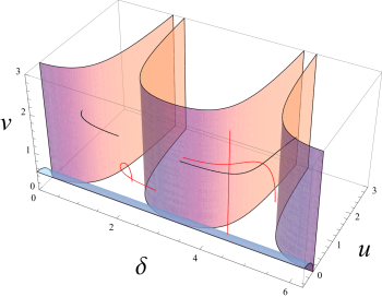
Figure 1: The black lines represent the trajectories associated to a points-Universe that bounce against the walls. Instead, the red lines describe the points-Universe witch directly approach the singularity.

We now implement a numerical integration of the system (LABEL:MCphitrans) in order to analyse the behaviour of the trajectories in the potential free region and then use this result for interpreting the effect of the scalar curvature. As we can see in the Fig.1 an opening of the domain emerges due to the presence of the scalar field and it is possible to individuate two families of trajectories: those ones corresponding to a point-Universe that bounces against the walls and turn back inside the domain (the black ones) and those corresponding to a particle that approach the so called “absolute”kirillov1997 (the red ones), for values $v\rightarrow 0,\infty$, with no other bounces until the singularity. The presence of the trajectories of the second family shows the removal of the oscillatory behavior of the Mixmaster model coupled with a massless scalar field BKLref2 ,berger . Let us see what happen if we consider the complete potential term(18). This time the restrictions on the dynamics imply that the particle is confined inside a region where all the six exponential terms in Eq.(18) are simultaneously greater than zero. We can immediately remove one of the six conditions because the first exponent related to the potential of the scalar field $1+u+u^{2}+v^{2}$ is always greater than zero for any values of $u,v$ taking in consideration. Thus, the five conditions that identify the domain are

$$\begin{cases}1+(1+2u)\cos\delta>0\\ 1-(1+2u)\cos\delta>0\\ u(u+1)+v^{2}>0\\ 1+u+u^{2}+v^{2}-2\sqrt{2\pi^{3}}(1+2u)\sin\delta>0\\ 1+u+u^{2}+v^{2}-4\sqrt{2\pi^{3}}(1+2u)\sin\delta>0\end{cases}$$ (23)

We observe that the last of the conditions above naturally implies the validity of the fourth one too. Thus, we indeed deal with four potential walls only. As we can see in the Fig.2, taking into account also the potential term $U(u,v,\delta,\tau)$ implies that the available configuration space for the point-Universe is clearly reduced with respect to the case $U=0$ (see Fig.1). However, trajectories yet exist(the red lines in the Fig.2) corresponding to a point-Universe that is able to reach the absolute for $v\rightarrow 0,\infty$. For this reason we can firmly conclude that a quadratic correction in the Ricci scalar to the Einstein-Hilbert action, that in the Scalar-Tensor theory is equivalent to the dynamics of a self-interacting scalar field (with potential terms of the form (7)), is able to remove the never-ending bounces of the point-Universe against the walls. As a result of the bounces against the infinite potential walls (which can be described by a reflection rulemontani-kirillov ,indicikasner ), soon or later the point-Universe reach a trajectory connected with the absolute. It is worth noting that the analysis above is referred to the choice $q>0$, in which case the sign of the scalar field potential is the same one of the scalar curvature. This choice is forced by the request that the additional scalar mode, associated to the quadratic modification, be a real (non-tachyonic) massive one, accordingly to the original Starobinsky approach in staro1 and demonstrated also in segnoq . However, in the case $q<0$, the scalar field potential would not contribute an infinite positive wall, but an infinite depression. Since in the region of zero potential, the point-Universe has always positive “energy”, we can easily conclude that such a case overlaps the non-chaotic potential-free one. We now observe that, in correspondence to the configuration region $v=0,\infty$ and $\delta=\frac{3\pi}{2}$, the scalar field acquires negative diverging values and its potential terms manifests a diverging behaviour. Such a profile of the scalar field is typical of a Bianchi I solution near the singularity scalar field and the diverging character of the potential term means that General Relativity can not be asymptotically recovered. Rigorously speaking, the present result on the chaos structure applies to a quadratic correction in the Ricci scalar only, because it is the first terms of the Taylor expansion of the function $f(R)$ working nearby the singularity. Nonetheless, our analysis has a general validity, as soon as, we take into account a physical cut-off at the Planck time, where classical theory starts to fail and a quantum treatment is required. In fact, the Planckian cut-off would remove the $\phi$ and $U(\phi)$ divergences, allowing the Taylor expansion for $q\lesssim\frac{(ct_{cut})^{2}}{l_{P}^{2}}$, where $t_{cut}$ being the cut-off time and $l_{P}$ the Planck length. Since $t_{cut}>\frac{l_{p}}{c}$, we deal with the (non-severe) restriction $q\lesssim 1$ for preserving the general nature of our result. This estimation follows requiring $R>qR^{2}$ and remembering that for the case of a Kasner solution, in the presence of a potential-free scalar field, the Ricci scalar behaves as $R\sim\frac{1}{t_{s}^{2}}$, where $t_{s}$ is the synchronous time. We stress that qualitatively, a similar argument is at the ground of the non-chaotic nature of the Bianchi IX Loop Quantum dynamics in the semi-classical limit boj . However, the field $\phi(t_{s})$ admits, both for $v\rightarrow 0,\infty$ and $\delta=\pi/2$, trajectories implying its positive divergence. For such behaviours, corresponding to an open region in the initial condition, the potential $U(\phi)$ approaches a constant value and $\phi$ is effectively massless. It is just the existence of these diverging profiles at the ground of the chaos removal in the present model. The massless nature of the potential along specific trajectories is a good criterion for determining the chaotic properties of the Mixmaster Universe in a specific non-expanded $f(R)$ model. In fact, The behavior of the free scalar field reads $\phi_{f}(t_{s})\propto\ln t_{s}$ and the corresponding kinetic energy density stands as $1/t_{s}^{2}$. Then, for a given $f(R)$ model, fixing the potential $U(\phi)$, the chaos removal is ensured by the validity of the condition $\lim_{t_{s}\rightarrow 0}U(\phi_{f}(t_{s}))t_{s}^{2}=0$. Clearly, the non-chaoticity is ensured if such a limit holds for a non-zero measure set of trajectories.

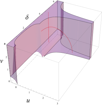
Figure 2: The point-Universe lives inside the region marked by the walls, where the conditions (23) are verified. We also sketch the trajectories reaching the absolute.

Conclusions

The analysis above demonstrated how including a quadratic correction in the Ricci scalar to the Einstein-Hilbert Lagrangian of the gravitational field gives a deep insight on the nature of the Mixmaster singularity: the evolution of the scale factors is no longer chaotic and a stable Kasner regime emerges as the final approach to the singular point.

The relevance of this result is in its generality with respect to the behaviour of the cosmological gravitational field. In fact, on one hand, the result we derived in the homogeneous cosmological setting, can be naturally extended to a generic inhomogeneous Universe, simply following the line of investigation discussed in BKLref2 ,scalar field .

The basic statement, at the ground of the BKL conjecture, is the space point decoupling in the asymptotic dynamics toward the cosmological singularity. Such a dynamical property of a generic inhomogeneous cosmological model allows to reduce the behavior of a sub-horizon spatial region BKLref2 ,M95 to the prototype offered by the homogeneous Mixmaster Universe. We are actually stating that the time derivative of the dynamical variables asymptotically dominate their spatial gradients, limiting the presence of the spatial coordinates in the Einstein equation to a pure parametrical role. We are speaking of a conjecture because the chaotic features of the point-like dynamics induce a corresponding stochastic behaviour of the spatial dependence and the statement above requires a non-trivial treatment for its proof. Nonetheless a valuable estimation of the spatial gradient behaviour, when the space-time takes the morphology of a foam, is provided in K93 . When a scalar field is present the situation is even more simple, because, after a certain number of iterations of the BKL map, in each space point, a stable Kasner regime takes place K87 and the validity of the solution is rigorously determined LK63 . Thus, we can extend our result to a generic inhomogeneous cosmological model simply considering the dynamical variables as space-time functions $u=u(\tau,x^{i})$, $v=v(\tau,x^{i})$ and $\delta=\delta(\tau,x^{i})$, which, in each space point, live in a half-Poincar space and are governed by an independent and morphologically equivalent dynamics. On the other hand, the extension of General Relativity we considered here is the most simple and natural one, widely studied in literatures in view of its implications on the primordial Universe features. Since the classical evolution is expected to be predictive up to a finite value of the Universe volume, i.e. up to a given amplitude of the space-time curvature, for sufficiently small coupling constant $q$ values, the present model can be considered as the quadratic Taylor expansion of a generic $f(R)$ theory and we can then guess that the non-chaotic feature is a very general dynamical property, at least within the classical domain of validity of the $f(R)$ theory. In this sense we traced a very general and reliable properties of the cosmological gravitational field in modified theories of gravity of significant impact on the so-called billiard representation of the generic primordial Universehennaux1 ,montani-kirillov ,indicikasner .

References

- (1) V.A. Belinskii, I.M. Khalatnikov, E.M. Lifshttz, Oscillatory approach to a singular point in the relativistic cosmology, Adv. Physics, 19(80), 525-573 (1970).
- (2) C. W. Misner, Mixmaster Universe, Phys. Rev. Letters 22, 1071, 1969).
- (3) C. W. Misner, Quantum Cosmology I, (PhysRev. 186, 1319, 1969).
- (4) V. A. Belinski, I. M. Khalatnikov and E. M. Lifshitz, A General Solution of the Einstein Equations with a Time Singularity, (Adv.Phys. 31, 639, 1982).
- (5) V. A. Belinskii, I. M. Khalatnikov, Effect of scalar and vector fields on the nature of the cosmological singularity, (Sov. Phys. JETP 36(4), 591-597 , 1973).
- (6) G. Montani, M. V. Battisti, R. Benini, G. Imponente, Classical and quantum features of the Mixmaster singularity, (International Journal of Modern Physics A 23, pp. 23532503, 2008).
- (7) G. Montani, M. V. Battisti, G. Imponente, R. Benini, Primordial cosmology, (World Scientific, 2011).
- (8) J. Demaret, M. Henneaux and P. Spindel, Phys. Lett., 164B, 27, (1985).
- (9) Y. Elskens and M. Henneaux, Nucl. Phys., B290, 111 (1987).
- (10) N. Deruelle and P. Spindel, Classical Quantum Gravity 7, 1599 (1990).
- (11) B. K. Berger, Influence of scalar fields on the approach to a cosmological singularity, (Physical Review D 61, 023508 , 1999).
- (12) Capozziello, S., Curvature Quintessence, Int. J. Mod. Phys. D 11 (2002) 483.
- (13) Capozziello, S., De Laurentis, M., Extended Theories of Gravity, Physics Reports 509 (2011) 167.
- (14) Nojiri, S., Odintsov, S.D., Unified cosmic history in modified gravity: from F(R) theory to Lorentz non-invariant models , Physics Reports 505 (2011) 59.
- (15) S. Nojiri, S. D. Odintsov, Introduction to Modified Gravity and Gravitational Alternative for Dark Energy, Int. J. Geom. Methods Mod. Phys. 04, 115 (2007)
- (16) Nojiri, S. and Odintsov, S. D. (2008). Dark energy, inflation and dark matter from modified f(r) gravity, arXiv:0807.0685
- (17) J.Q. Guo, D. Wang, and A. V. Frolov, Phys. Rev. D 90, 024017 (2014).
- (18) J. D. Barrow and S. Cotsakis, Phys. Lett. B, 232, 172-176 (1989).
- (19) J. D. Barrow and H. Sirousse-Zia, Phys. Rev. D, 39, 2187-92 (1989).
- (20) J. D. Barrow and S. Cotsakis, Phys. Lett. B, 214, 515-518 (1988).
- (21) N. Deruelle, Nucl. Phys. B327 253 (1989)
- (22) Starobinsky, A. A. (1980). A new type of isotropic cosmological models without singularity. Physics Letters B 91 99-102.
- (23) P. A. R. Ade et al. [Planck Collaboration] ,Planck 2013 results. XXII. Constraints on inflation, arXiv:1303.5082 [astro-ph.CO]
- (24) Misner, C. W., K. S. Thorne, and J. A. Wheeler, 1973, Gravitation (Freeman Press, San Francisco).
- (25) G. Montani, A. A. Kirillov, Origin of a classical space in quantum inhomogeneous models, (Zh. ksp. Teor. Fiz. 66, No. 7, 449-453 ,1997).
- (26) G. P. Imponente, G. Montani, On the covariance of the mixmaster chaoticity, (Physical Review D 63, p. 103501, 2001).
- (27) R. Arnowitt, S. Deser, C. W. Misner, Canonical variables for general relativity, (Physical Review 117, 6, pp. 1595-1602, 1959).
- (28) Pesin Ya B (1977) UMN (Russian Mathematical Surveys), Lyapunov Characteristic Numbers and Smooth Ergodic Theory 32, n.4 55-112
- (29) V. I. Arnold, Mathematical Methods of Classical Mechanics, Springer-Verlag (1989)
- (30) Chitré D. M. (1972) Ph.D. Thesis, University of Maryland
- (31) A. A. Kirillov, G. Montani (1997) Phys. Rev. D, 56, n.10, 6225.
- (32) I. M. Khalatnikov and E. M. Lifshitz, Phys. Rev. Lett. 24, 76 (1970).
- (33) T. Damour, O. M. Lecian, Statistical Properties of Cosmological Billiards, Phys. Rev. D, 83 044038, (2011).
- (34) S. Capozziello and S. Vignolo, The Cauchy problem for metric-affine f(R)-gravity in presence of perfect-fluid matter, Class. Quant. Grav. 26 (2009) 175013
- (35) Bojowald, M., Date, G. and Hossain, G. M. (2004). The Bianchi IX model in loop quantum cosmology, Class.Quant.Grav. 21, pp. 35413570
- (36) S. Capozziello and S. Vignolo, The Cauchy problem for metric-affine f(R)-gravity in presence of perfect-fluid matter, Class. Quant. Grav. 26 (2009) 175013
- (37) G.Montani On the General Behaviour of the Universe Near Cosmological Singularity, Classical and Quantum Gravity, 12, 2503, (1995).
- (38) Kirillov, A. A. On the question of the characteristics of the spatial distribution of metric inhomogeneities in a general solution to einstein equations in the vicinity of a cosmological singularity, Soviet Physics JETP 76, p. 355., (1993).
- (39) Kirillov, A. A. and Kochnev, A. A. (1987). Cellular structure of space in the vicinity of a time singularity in the einstein equations, Pis ma Zhurnal Eksperimental noi i Teoreticheskoi Fiziki 46, pp. 345?348.
- (40) E.M. Lifshitz, I.M. Khalatnikov, Investigations in relativistic cosmology, Adv. Physics, 12(46), 185-249 (1963