Looking for Integrability on the Worldsheet of Confining Strings

Patrick Cooper^a, Sergei Dubovsky^a,b, Victor Gorbenko^a,
Ali Mohsen^a, and Stefano Storace^a
aCenter for Cosmology and Particle Physics,
Department of Physics, New York University
New York, NY, 10003, USA
^bAbdus Salam International Center for Theoretical Physics,
Strada Costiera 11, 34151, Trieste, Italy

We study restrictions on scattering amplitudes on the worldvolume of branes and strings (such as confining flux tubes in QCD) implied by the target space Poincaré symmetry. We focus on exploring the conditions for the string worldsheet theory to be integrable. We prove that for a higher dimensional membrane the scattering amplitudes for the translational Goldstone modes (“branons”) are double soft. At one-loop double softness is generically violated for the string worldsheet scattering as a consequence of collinear singularities. Violation of double softness implies in turn the breakdown of integrability. We prove that if branons are the only gapless degrees of freedom then the worldsheet integrability is compatible with target space Poincaré symmetry only if the number of space-time dimensions is equal to $D=26$ (a critical bosonic string), and for $D=3$. We extend the analysis to include massless worldsheet fermions, resulting from spontaneous breakdown of the target space supersymmetry. We check that the tree-level integrability in this case is in one-to-one correspondence with the existence of a $\varkappa$-symmetric Green-Schwarz (GS) action. As a byproduct we show that at the leading order in the derivative expansion an $\mathcal{N}=1$ superstring without $\varkappa$-symmetry in $D=3,4,6,10$ dimensions exhibits an accidental enhanced supersymmetry and is equivalent to a $\varkappa$-symmetric $\mathcal{N}=2$ GS superstring.

1 Introduction

String theory was born as a model of strong interactions [1], and this is not a coincidence. The stringy nature of hadrons is convincingly proven both by linearly rising Regge trajectories (see, e.g., [2] for a recent compilation of meson spectra), and by lattice simulations. Nevertheless the theory of the QCD confining string (also known as the flux tube) still remains elusive.

Remarkable progress in this direction was achieved recently for the $\mathcal{N}=4$ supersymmetric cousin of QCD, where it turned out to be possible to find an exact integrable S-matrix on the flux tube worldsheet, allowing one to solve the theory in the planar limit (for a review, and more precise explanation of what “solve” means here, see [3]; for most recent developments and further later references see, e.g., [4]). Note, however, that $\mathcal{N}=4$ supersymmetric Yang–Mills (SYM) is a conformal theory, and as such does not possess confining flux tubes in a strict sense. Instead, in this case it is more appropriate to think about strings in the dual $AdS_{5}\times S^{5}$ space.

In addition, an approximate low energy integrability of the worldsheet theory proved to be a powerful perturbative tool for calculating the spectra of confining strings in non-supersymmetric gluodynamics [5, 6]. This new technique allowed for a solid theoretical interpretation of the available high quality lattice data [7, 8], and lead to the identification of the first massive excited state on the worldsheet of the QCD string.

Of course, there is no reason to expect the worldsheet theory of the confining string in real world QCD to be integrable. However, given the integrability of the $\mathcal{N}=4$ SYM string it is tempting to look for genuinely confining theories with less supersymmetries enjoying integrability on the flux tube worldsheet, at least in the planar limit.

The goal of the present paper is to take a small step in this direction, by identifying necessary conditions for integrability of the flux tube theory. We take a bottom up approach and study the constraints on the low energy worldsheet scattering imposed by the Poincaré symmetry of the full theory.

In section 2 we start with a few general remarks about the properties of worldvolume scattering amplitudes for branes embedded into Minkowski space-time. From an effective field theory point of view, a brane may be thought of as a system of Goldstone bosons—branons, corresponding to the spontaneous breaking of translational invariance. We prove that for a generic number of worldvolume dimensions the branons’ amplitudes are doubly soft—in the limit when one of the scattering branons is soft, the amplitude vanishes as the second power of its energy. This is a natural extension of the conventional soft pion theorems.

In section 3 we study whether worldsheet integrability is possible when branons are the only gapless worldsheet degrees of freedom. In other words, at low energies a flux tube is described by a Nambu–Goto bosonic string in this case. Then integrability is always present at the tree-level. The key observation behind our analysis is that string worldsheet amplitudes are universal not only at tree-level, but also at one-loop [9]. By direct inspection of one-loop scattering we find that integrability is broken unless the string is critical, $D=26$, or the dimensionality of the target space-time is $D=3$. This breakdown of integrability can be traced to the violation of the double softness property, as a consequence of collinear singularities contributing to the corresponding Ward identities. This proves the following no-go theorem:

Worldsheet scattering on the confining flux tube of a four-dimensional gauge theory can be integrable only in the presence of additional gapless degrees of freedom.

In section 4 we consider whether the no-go theorem may be avoided by introducing additional massless degrees of freedom on the worldsheet. Here we restrict to the simplest possibility, namely, we add goldstini—fermions which are massless as a consequence of non-linearly realized target space supersymmetry. We find that in this case even tree-level integrability is not guaranteed any longer. If all supercharges are broken, tree level integrability holds only for $\mathcal{N}=1$ supersymmetry in space-time dimensionalities $D=3,4,6,10$. These are the dimensionalities where the $\varkappa$-symmetric Green–Schwarz (GS) superstring action can be constructed [10]. The GS superstring does exhibit unbroken supercharges and is integrable at tree level both for $\mathcal{N}=1$ and $\mathcal{N}=2$.

This analysis makes slightly more precise the standard lore that classical superstrings exist only for the above special choices for the number of space-time dimensions and supercharges. This cannot be literally correct, given that at the effective field theory level one clearly can construct string actions corresponding to an arbitrary choice of supersymmetric coset. The accurate statement is that a classically integrable superstring action exists only for $\mathcal{N}=1,2$ and $D=3,4,6,10$. As for the bosonic string, the classical integrability survives at the quantum level only for the critical superstrings $D=10$, or at $D=3$.

As a byproduct of this analysis we also prove the following. In principle, for $\mathcal{N}=1,2$ and $D=3,4,6,10$ one can construct a continuous family of inequivalent superstring actions, parameterized by the coefficient $c$ in front of the Wess-Zumino (WZ) term. For the standard GS choice $c=\pm 1$ the theory enjoys an additional fermionic gauge symmetry—the famous $\varkappa$-symmetry [11]. For $\mathcal{N}=2$ and $c\neq\pm 1$ we find that the classical integrability is lost, which could have been expected. However, somewhat surprisingly, for $\mathcal{N}=1$ we find that the theory is integrable for all values of $c$. On-shell amplitudes are independent of $c$, and the model exhibits an additional hidden supersymmetry. In other words, $\mathcal{N}=1$ models without $\varkappa$-symmetry are equivalent to gauge fixed $\varkappa$-invariant $\mathcal{N}=2$ GS models. A similar observation for superparticles has been made recently in [12].

In section 5 we conclude and discuss future directions.

2 Current Algebra for Branes

The main focus of our paper is to study the consistency of integrability with the non-linearly realized target space Poincaré symmetry on the string worldsheet. However, it is instructive to start with a few general observations on the implications of the target space Poincaré symmetry for the brane worldvolume scattering.

There are two general methods to impose conditions of a non-linearly realized symmetry on scattering amplitudes. First, one may follow the coset construction [13] to build the Goldstone action invariant under the full symmetry group. Scattering amplitudes constructed from this action are guaranteed to satisfy the required Ward identities. For non-linearly realized space-time symmetries the corresponding construction has been worked out in [14, 15, 16]. At the leading order in the derivative expansion it gives rise to the Nambu–Goto (NG) action for a $p$-brane,

$$S_{NG}=-\ell_{s}^{-p-1}\int d^{p+1}\sigma\sqrt{-\det\left({\eta_{\alpha\beta}+\ell_{s}^{p+1}\partial_{\alpha}X^{i}\partial_{\beta}X^{i}}\right)}\;,$$ (1)

where $\sigma^{\alpha}$, $\alpha=0,\dots,p$ are the worldvolume coordinates, $\eta_{\alpha\beta}$ is the worldvolume Lorentz metric, and $X^{i}$, $i=p+1,\dots,D$ are physical transverse excitations of the brane (“branons”). Finally, $\ell_{s}$ is the brane width, so that the tension is equal to $\ell_{s}^{-p-1}$.

This method is very physical and constructive, but it does not make immediately manifest special properties of the scattering amplitudes following from the non-linearly realized symmetry. For example, the vanishing of the QCD scattering amplitudes in the limit when any of the external pion legs become soft (a single soft pion theorem) is not immediate to see from the pion chiral Lagrangian. The approach which allows one to directly see various soft theorems goes under the name of current algebra (see, e.g., [17] for a review). The main idea is to systematically study the Ward identities for the spontaneously broken currents.

Let us apply this method to brane worldvolume scattering and derive the analogue of the single soft pion theorem in this case. Note that, unlike for the pion chiral Lagrangian, every Goldstone field appears in (1) with a derivative acting on it. This is related to the trivial commutation relations between spontaneously broken generators of translations and makes the conventional single soft property of the branon scattering amplitudes obvious already at the level of the action. However, one may expect more. Indeed, the conventional soft pion theorems reflect the existence of a continuous family of vacua related by the action of broken symmetry generators (see, e.g., [18] for a recent discussion). For a brane the moduli space is even larger and includes the possibility of tilting the brane and moving it with a constant velocity, i.e., includes configurations like $X^{i}=v^{i}_{\alpha}\sigma^{\alpha}$. This property is also related to the fact that one branon is responsible for a few broken symmetries—shifts, rotations and boosts. This gives rise to the expectation of an even stronger softness property for branon amplitudes. This intuition can be converted into a more rigorous current algebra argument as follows.

Spontaneously broken translations of the target space give rise to conserved shift currents $S_{\alpha}^{i}$, which take the form

$$S_{\alpha}^{i}=\ell_{s}^{1-p\over 2}\partial_{\alpha}X^{i}+s_{\alpha}^{i}\;,$$ (2)

where $s_{\alpha}^{i}$ is the non-linear part of the current. In the same way as for pions, the existence of these currents implies that the scattering amplitudes for the emission of a branon are soft, i.e., they vanish in the limit $p^{\alpha}\to 0$, where $p^{\alpha}$ is the branon momentum. However, branon amplitudes have additional non-obvious softness properties following from the existence of spontaneously broken boost currents $J_{\alpha}^{i\beta}$. The general form for these is

$$J_{\alpha}^{i\beta}=\ell_{s}^{-1}(\sigma^{\beta}S^{i}_{\alpha}-K_{\alpha}^{i\beta})\;,$$ (3)

where $K_{\alpha}^{i\beta}$ have no explicit dependence on the world-volume coordinates. Conservation of the boost currents implies that the shift current is itself a total derivative on shell,

$$S^{i}_{\alpha}=\partial_{\beta}K_{\alpha}^{i\beta}$$ (4)

or, equivalently,

$$s^{i}_{\alpha}=\partial_{\beta}k_{\alpha}^{i\beta}\;,$$ (5)

where $k_{\alpha}^{i\beta}$ is again the piece of $K_{\alpha}^{i\beta}$ which depends non-linearly on the fields. To extract the consequences of non-linearly realized boosts one may either study Ward identities involving boost currents, or make use of (4) in the Ward identities for the shift current itself. We will follow the latter path.

Note that it is straightforward to check (4) for the NG action explicitly, and also to find the explicit form for the operator $K_{\alpha}^{i\beta}$ in this case. Indeed, the only dependence of the NG action on the worldvolume Lorentz metric $\eta_{\alpha\beta}$ is through the induced metric

$$\gamma_{\alpha\beta}=\eta_{\alpha\beta}+\ell_{s}^{p+1}\partial_{\alpha}X^{i}\partial_{\beta}X^{i}\;.$$

Hence, variation of the action under coordinate-dependent shifts

$$X^{i}\to X^{i}+\ell_{s}^{1-p\over 2}\epsilon(\sigma)$$

as required for deriving the Noether shift current, is equivalent to the change of the metric according to

$$\eta_{\alpha\beta}\to\eta_{\alpha\beta}+\ell_{s}^{3+p\over 2}(\partial_{\alpha}\epsilon\partial_{\beta}X^{i}+\partial_{\beta}\epsilon\partial_{\alpha}X^{i})\;.$$

As a result one obtains

$$S_{\alpha}^{i}=\ell_{s}^{3+p\over 2}\partial_{\beta}X^{i}T^{\beta}_{\alpha}\;,$$ (6)

where $T^{\beta}_{\alpha}$ is the world-volume energy-momentum tensor. As a consequence of the conservation of $T^{\beta}_{\alpha}$, the relation (4) follows from (6) on shell with

$$K_{\alpha}^{i\beta}=\ell_{s}^{3+p\over 2}X^{i}T^{\beta}_{\alpha}\;.$$ (7)

Let us now study the consequences of the non-linearly realized Poincaré symmetry by inspecting matrix elements with a single insertion of the shift current in the form (4). In this case the reasoning goes very similar to the standard pion current algebra arguments. Namely, one starts with the current conservation written in the form

$$\langle out|\partial^{\alpha}S^{i}_{\alpha}|in\rangle=0\;.$$

By performing the Fourier transform and making use of (2), (5) we obtain

$$\ell_{s}^{1-p\over 2}p^{2}\langle out|X^{i}(p)|in\rangle+p^{\alpha}p_{\beta}\langle out|k_{\alpha}^{i\beta}(p)|in\rangle=0\;.$$ (8)

The matrix element entering the first term in (8) has a one branon LSZ pole at $p^{2}=0$, while the second matrix element is in general regular at $p^{2}=0$. Consequently, restricting to the case $p_{0}>0$ and taking the limit $p^{2}\to 0$, we obtain

$$i\ell_{s}^{1-p\over 2}\langle out|in,p\rangle=-p^{\alpha}p_{\beta}\langle out|k_{\alpha}^{i\beta}(p)|in\rangle\;,$$ (9)

where $|in,p\rangle$ is the initial state with an additional branon of momentum $p$. By taking now the soft limit $p^{\alpha}\to 0$ we conclude that non-linearly realized Poincaré symmetry implies that scattering amplitudes with a single soft branon emission are double soft, i.e. they vanish as a second power of the branon momentum. Let us stress that the underlying assumption for this argument is that matrix elements of $k_{\alpha}^{i\beta}$ are regular functions of $p^{\alpha}$. For a general $p$-brane this should be the case, because $k_{\alpha}^{i\beta}$ is a non-linear operator, however, we will see later that there is an interesting subtlety in the string case, $p=1$.

3 Bosonic Strings

Let us specialize now to the $p=1$ case, i.e. consider scattering on the worldsheet of a string. Let us first consider the case when the translational Goldstones $X^{i}$ are the only massless degrees of freedom. Their $SO(D-2)$-symmetric $2\to 2$ amplitude can be conveniently parameterized in terms of three functions $A$, $B$, and $C$ called respectively annihilations, transmissions and reflections,

$${\cal M}_{ij,kl}=A\delta_{ij}\delta_{kl}+B\delta_{ik}\delta_{jl}+C\delta_{il}\delta_{jk}\>.$$ (10)

For $2\to 2$ scattering in two dimensions the momentum transfer between particles is impossible, hence one can always choose $p_{1}=-p_{3}$ and $p_{2}=-p_{4}$, which in terms of Mandelstam variables reads

$$-(p_{1}+p_{2})^{2}=s=-u,\qquad t=0$$ (11)

Thus, effectively the amplitude is a function of only one variable. In what follows we consider massless particles and it is convenient to distinguish left-movers with non-zero $p_{+}\equiv{(p_{0}+p_{1})/\sqrt{2}}$ and right-movers with non-zero $p_{-}\equiv{(p_{0}-p_{1})/\sqrt{2}}$. Crossing symmetry relates $A$, $B$ and $C$ as

$$A(s)=C(-s),\quad B(s)=B(-s).$$ (12)

In particular, the absence of reflections is equivalent to the absence of annihilations. At tree-level the worldsheet $S$-matrix of the bosonic string is integrable and reflectionless in any number of dimensions. A short proof of this statement goes as follows. Let us consider the light-cone quantization of the bosonic string. At the classical level the light-cone gauge is perfectly consistent with all the symmetries, hence tree-level worldsheet amplitudes should be correctly reproduced by this quantization for any number of space-time dimensions. The light-cone energy levels depend only on the total left- and right-moving momenta of a state (“levels” of a string state) and depend neither on how these momenta are distributed among individual particles, nor on the $SO(D-2)$ quantum numbers of the state. This implies that there is no particle production and that the scattering is reflectionless. Then, to specify the full tree-level $S$-matrix, one only needs the transmission part of the $2\to 2$ amplitude, which reads

$$B_{tree}=\frac{\ell_{s}^{2}}{2}s^{2}\ .$$ (13)

Furthermore, the non-linearly realized Poincaré symmetry forbids any term in the action that can contribute at one-loop level to the on-shell $S$-matrix elements, thus also making the one-loop $S$-matrix universal and uniquely specified by symmetries.

The one-loop calculation of $2\to 2$ scattering was performed in [9], where it was found that the reflectionless property of the S-matrix is violated due to the presence of a finite rational term in the amplitude, unless the number of dimensions is equal to 26,

$$A_{1-loop}=-C_{1-loop}=-\frac{D-26}{192\pi}\ell_{s}^{4}s^{3}\ .$$ (14)

Also the $D=3$ case is special, in this case there is only one flavor, making the notion of annihilations meaningless, and the rational term in the amplitude vanishes as a consequence of $A+C=0$.

Even though the $2\to 2$ scattering is always integrable in two dimensions due to purely kinematic reasons, this result shows that the $S$-matrix cannot be integrable already at the level of $3\to 3$ scattering in non-critical bulk dimensions larger than four. The reason is that in an integrable theory $3\to 3$ $S$-matrix elements must satisfy the Yang-Baxter equation (see, e.g., [22] for an introduction). The Yang-Baxter equation can be understood as the condition on an integrable $S$-matrix coming from the fact that the order in which the two-particle scatterings occur does not affect the multi-particle $S$-matrix,

$$S_{ij}^{kl}S_{km}^{np}=S_{im}^{kp}S_{kj}^{nl}.$$ (15)

When the number of flavors is larger than two it cannot be satisfied in the presence of reflections and annihilations. To see this, note that for three distinct flavors $i$, $j$ and $k$, the process $X^{i}(p_{-})X^{j}(q_{-})X^{j}(p_{+})\to X^{i}(p_{+})X^{k}(p_{-})X^{k}(q_{-})$ (Figure 1, left) is possible, while the $X^{j}(q_{-})X^{i}(p_{-})X^{j}(p_{+})$ state can only evolve into $X^{k}(p_{+})X^{k}(q_{-})X^{i}(p_{-})$ state if one demands that $X^{j}$ particles annihilate (Figure 1, right).

Figure 1: Yang-Baxter equation cannot be satisfied in the $SO(N)$-symmetric massless theory in the presence of reflections for $N>2$

This argument, however, does not go through for two flavors. By considering all possible 3$\to$3 processes in $SO(2)$ symmetric theories we get the following condition from the Yang–Baxter equation

$$A(s)=-C(s),$$ (16)

Note that the one-loop amplitude (14) satisfies this relation.

It is interesting to construct an example of an exact $S$-matrix satisfying this condition as well as the usual requirements of unitarity and analyticity. These conditions are more naturally formulated in terms of the $S$-matrix elements rather than amplitudes. We will denote them by

$$a(s)=i\frac{A(s)}{2s},\quad b(s)=1+i\frac{B(s)}{2s},\quad c(s)=i\frac{C(s)}{2s},$$ (17)

where denominators are coming from the relativistic normalization for scattering states. Then real analyticity requires $a(s)^{\dagger}=a(s^{\dagger})$ and the same for $b$ and $c$. All these functions have a cut going all the way along the real axis. Finally, unitarity imposes the following independent constraints

$$bb^{\dagger}+aa^{\dagger}=1,\quad ba^{\dagger}+b^{\dagger}a=0,$$ (18)

Combining real analyticity, (12), (16) and (18) we get the following equation for the ratio of $a$ and $b$

$$\frac{a(s)}{b(s)}=\frac{a(-s)}{b(-s)}=\sqrt{\frac{b(s)b(-s)-1}{b(s)b(-s)}},$$ (19)

where we now understand $a$ and $b$ to be the meromorphic functions obtained by analytic continuation from the physical sheet.

The simplest solution to this equation is

$$b = \cos 2\phi\frac{\left(s-\frac{i\rho}{\sqrt{\cos 2\phi}}\right)^{2}}{\left(s+i\rho{\rm e}^{i\phi}\right)\left(s+i\rho{\rm e}^{-i\phi}\right)},$$ (20)

$$a = i\sin 2\phi\frac{s^{2}\left(s-\frac{i\rho}{\sqrt{\cos 2\phi}}\right)^{2}}{\left(s+\frac{i\rho}{\sqrt{\cos 2\phi}}\right)\left(s+i\rho{\rm e}^{i\phi}\right)\left(s+i\rho{\rm e}^{-i\phi}\right)}$$ (21)

In order to avoid poles on the physical sheet (i.e., at ${\rm Im}\;s>0$) $\phi$ should be in the interval $\phi\in[-\pi/4,\pi/4]$. Other examples can be produced by multiplying this $S$-matrix by CDD factors (cf.,[23]).

To see whether there is a chance for a massless $O(2)$ invariant integrable theory of this kind to exhibit the full four-dimensional Poincaré symmetry, let us inspect one-loop six-particle on-shell amplitudes following from the NG action. Just like one-loop four-particle amplitudes, these are universal as long as branons are the only massless degrees of freedom. Consequently, if some one-loop six-particle amplitude does not vanish in non-integrable kinematics, integrability requires extra gapless modes on a flux tube in four dimensions.

It is a matter of a straightforward (even if a bit tedious) calculation to find out how these amplitudes look. We use dimensional regularization to preserve the non-linearly realized Poincaré invariance. As shown in Figure 2, diagrams of three different topologies contribute to the answer. For the sake of generality we explore the amplitude for a general target space dimensionality. There are two different types of kinematics allowed for the processes involving six particles: two left-movers and four right-movers (or vice-versa) and three left-movers and three right-movers. We skip the details of the calculation, and only present the results here. The most subtle part of this calculation is the treatment of the Feynmann integrals corresponding to the triangle graph in Figure 2. We present the corresponding details in the Appendix.

When the dust settles, it turns out that for non-integrable kinematics (i.e., in the presence of a non-trivial momentum redistribution between left- and/or right-movers) processes of the first type have vanishing amplitudes. However, we find that amplitudes with three right-movers and three left-movers (which necessarily violate integrability) do not vanish, unless the string is critical, $D=26$, or for $D=3$. To present the final answer in a compact form it is instructive to start with a few general remarks about the possible structure of the amplitude.

The NG theory is integrable at the classical level. Moreover, for any $D$ one can construct an integrable $S$-matrix, characterized by a two particle phase shift [20],

$${\rm e}^{2i\delta_{GGRT}(s)}={\rm e}^{is\ell_{s}^{2}/4}\;,$$ (22)

which agrees with the NG theory at the classical level. Here GGRT stands for Goddard, Goldstone, Rebbi and Thorn [24] because for any $D$ this $S$-matrix corresponds to the light-cone quantization of the bosonic string. This implies that at the leading order in the derivative expansion the difference between relativistic NG amplitudes and the GGRT amplitude (22) should be a rational term, i.e. it should be possible to write a local vertex reproducing the corresponding amplitude. Indeed, the $S$-matrix (22) satisfies all analyticity, unitarity etc. requirements and weakly coupled at low energies. Hence, one should be able to write a local Lagrangian, which perturbatively reproduces it order-by-order in the derivative expansion. At the leading order this is the NG Lagrangian. If the latter gives a different answer from (22) at a certain order, the difference can be canceled by local counterterms.

For instance, the one-loop two particle annihilation amplitude discussed above can be reproduced from the following local vertex,

$${\cal L}_{4}=\ell_{s}^{4}{D-26\over 48\pi}\partial_{+}^{2}X^{i}\partial_{-}^{2}X^{i}\partial_{+}X^{j}\partial_{-}X^{j}\;.$$ (23)

Then for the non-integrable part of the six particle amplitude we find that it corresponds to the following local vertex,

$${\cal L}_{6}=\ell_{s}^{6}{D-26\over 48\pi}\partial_{+}^{2}X^{i}\partial_{-}^{2}X^{i}\left((\partial_{+}X^{j}\partial_{-}X^{j})^{2}-{1\over 2}\partial_{+}X^{j}\partial_{+}X^{j}\partial_{-}X^{k}\partial_{-}X^{k}\right)\;.$$ (24)

Figure 2: Diagrams contributing to the one-loop branon 6-point function

Both terms in (24) encode a number of different processes related by crossing symmetry and violating integrability. For instance, the first one gives rise to $2\to 4$ scattering of the following flavor structure

$$X^{i}(p_{+}+q_{+})X^{i}(p_{-}+q_{-})\to X^{j}(p_{+})X^{j}(p_{-})X^{k}(q_{+})X^{k}(q_{-})\;,$$ (25)

the corresponding scattering amplitude is

$${\cal M}^{(1)}_{2\to 4}=\ell_{s}^{6}\frac{D-26}{24\pi}p_{-}q_{-}(p_{-}+q_{-})p_{+}q_{+}(q_{+}+p_{+})(p_{+}(2p_{-}+q_{-})+q_{+}(2q_{-}+p_{-}))\;.$$ (26)

Diagrammatically, the only non-vanishing contribution to this process comes from the triangle graphs in Figure 2.

The second term in (24) contributes, for example, into

$$X^{i}(p_{+}+q_{+})X^{i}(p_{-}+q_{-})\to X^{j}(p_{+})X^{j}(q_{+})X^{k}(p_{-})X^{k}(q_{-})\;.$$ (27)

In this case graphs of all three topologies contribute, and the result is

$${\cal M}^{(2)}_{2\to 4}=-\ell_{s}^{6}\frac{D-26}{24\pi}p_{+}q_{+}p_{-}q_{-}(p_{+}+q_{+})^{2}(p_{-}+q_{-})^{2}\;.$$ (28)

For $D=4$ the effective non-integrable vertex (24) simplifies and takes the following form

$${\cal L}_{6,4d}=\ell_{s}^{6}{D-26\over 48\pi}\left(\partial_{+}^{2}{X^{\dagger}}\partial_{-}^{2}X\left(\partial_{-}{X^{\dagger}}\partial_{+}X\right)^{2}+h.c.\right)\;,$$ (29)

where $X=(X^{1}+iX^{2})/\sqrt{2}$. This completes the proof of the no-go theorem formulated in the Introduction. The effective vertex (29) gives rise, for instance, to the following non-integrable process

$${X^{\dagger}}(p_{+}+q_{+})X(p_{-}+q_{-})\to X^{\dagger}(p_{+})X^{\dagger}(q_{+}){X}(p_{-}){X}(q_{-})\;,$$

and the corresponding amplitude is

$${\cal M}^{4d}_{2\to 4}=\ell_{s}^{6}\frac{11}{6\pi}p_{-}q_{-}p_{+}q_{+}(p_{-}+q_{-})^{2}(p_{+}+q_{+})^{2}.$$ (30)

We see that if the branons are the only massless particles on a string, the classical integrability is necessarily broken unless the string is critical, $D=26$, or there is a single branon, $D=3$, since in this case $X^{\dagger}=X$ and (29) vanishes on shell. In these two special cases we know the exact $S$-matrix describing the corresponding integrable theory, it is determined by the GGRT phase shift (22). Indeed, in both cases the light-cone quantization is compatible with nonlinearly realized Lorentz symmetry. It remains to be seen whether a consistent interacting $D=3$ string theory can be constructed. Even if this is the case, it appears unlikely that it could be realized on the worldsheet of a confining string of some conventional three-dimensional gauge theory. The reason is that the corresponding short strings (i.e., strings with zero winding), which would correspond to glueballs, are anyons with irrational spins [25] at $D=3$. It would be surprising if one could obtain such a spectrum in the large $N$ limit of some gauge theory, although it is definitely interesting to understand whether the $D=3$ free string can be promoted into an interacting theory.

3.1 Current Algebra for Strings

A peculiar and somewhat surprising property of the amplitudes (26), (28) and (30) is that they violate current algebra relations derived in Section 2. Namely, they are not double soft with respect to all external momenta. What happens is that in two dimensions the right hand side of (9) can develop a singularity when $p^{\alpha}$ goes to zero for generic values of other momenta. The basic technical reason is that collinear singularities may be present for a generic kinematics in two dimensions.

Note that one might be surprised that we did not encounter IR singularities before. Indeed, the standard lore says that “there are no Goldstone bosons in two dimensions” [26], and, more generally, massless two dimensional theories are plagued with IR singularities. However, the string worldsheet theory provides a counterexample to this statement. We just saw that on-shell worldsheet scattering amplitudes do not show any signs of IR divergencies, and the exact $S$-matrix of a critical string (22) illustrates that there is no reason to expect IR divergencies at higher loops.

Of course, technically the arguments presented in [26] are all correct, however they only prove that Goldstone fields $X^{i}$ do not give rise to well defined operators in a quantum theory. In the string action there is always at least one derivative acting on every $X^{i}$. This is enough to ensure the absence of IR divergencies in on-shell scattering amplitudes. On the other hand, the non-linear part of the boost current (7) contains a Goldstone field without a derivative acting on it, so it is not surprising that IR divergencies appear in the Ward identities for this current. In general, we expect that such singularities are related to lower order amplitudes and matrix elements of some operators through unitarity, consequently the corrected Ward identities and soft theorems can be constructed.

Let us illustrate now how this works using one-loop six particle amplitudes with all flavors $i,j,k$ different, which we already calculated by brute force, as an example. Then the most natural place for collinear singularities to appear in (9) is through the diagrams of the type shown in Figure 3. Indeed, for concreteness, let us choose the soft momentum to be left moving, $p_{-}=0$. Then if all the external legs of the operator $k_{\alpha}^{i\beta}(p)$ are right moving, the internal line connecting $k_{\alpha}^{i\beta}(p)$ to the rest of the diagram goes on-shell in the soft limit, $p_{+}\to 0$, leading to an IR singularity.

Actually, one might worry that a collinear singularity could be present even before taking the soft limit, if all the external legs of the operator $k_{\alpha}^{i\beta}(p)$ are left moving. This would invalidate the transition from the off-shell current conservation (8) to the on-shell relation (9). To see that this does not happen, note that at the order we are working we may make use of (7) and write

$$p^{\alpha}p_{\beta}k_{\alpha}^{i\beta}=p_{+}^{2}X^{i}\tau_{--}+2p_{+}p_{-}X^{i}\tau_{+-}+p_{-}^{2}X^{i}\tau_{++}\;,$$ (31)

where $\tau_{\alpha\beta}$ is the energy-momentum tensor for $(D-2)$ free bosons. In the on-shell limit $p_{-}\to 0$ the collinear singularity from the internal line in Figure 3 scales as $p_{-}^{-1}$. Then, given that $\tau_{+-}=0$ for free bosons, only the first term in (31) survives on-shell. Finally, for this term to contribute, at least one of the external legs attached to it should be right moving. We see that one can safely use (9) and, moreover, $p^{\alpha}p_{\beta}k_{\alpha}^{i\beta}(p)$ reduces just to $p_{+}^{2}k_{--}^{i}$.

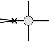
Figure 3: A collinear singularity present in the shift current Ward identity

Furthermore in the soft limit, $p_{+}\to 0$, we can write

$$\langle out|k_{--}^{i}(p_{+})|in\rangle=\sum_{j_{1},j_{2},k}i{\cal N}_{3}(p_{-j_{1}},p_{-j_{2}})\times\frac{i}{2p_{+}(p_{-j_{1}}+p_{-j_{2}})}\times i{\cal M}_{4}((p_{-j_{1}}+p_{-j_{2}})_{k})+reg.$$ (32)

Here the sum goes over all possible right-movers $j_{1},j_{2}$ entering in $|in\rangle$, $|out\rangle$ and over all possible right-movers $k$, which combined with $j_{1}$, $j_{2}$, produce a non-vanishing matrix element ${\cal N}_{3}(p_{-i},p_{-j})$ for the operator $k_{--}^{i}(0)$. ${\cal M}_{4}((p_{-j_{1}}+p_{-j_{2}})_{k})$ is a four particle scattering amplitude between the state $k$ (carrying the momentum $(p_{-j_{1}}+p_{-j_{2}})$) and the remaining particles in $|in\rangle$, $|out\rangle$. Finally, $reg.$ stands for terms non-singular in the soft limit.

Singular terms in (32) imply violation of the double softness property of the amplitude. We see that Ward identities in this case do not imply that the amplitude is double soft, but rather determine the single-soft piece of the amplitude through the amplitude with a smaller number of particles and a three-particle matrix element of $k_{--}^{i}(0)$. As follows from (7), to determine a singular piece we may replace this operator by $\ell_{s}^{2}X^{i}\partial_{-}X^{j}\partial_{-}X^{j}$. This is true also for amplitudes with a larger number of external states, since by Lorentz invariance the parts of $k_{--}^{i}$ containing more than three fields will necessarily introduce positive powers of $p_{+}$.

Furthermore, for the kinematics with three left-movers and three right-movers, which we considered in our brute force calculation, the most general effective vertex is a sum of two terms of the form present in (24). Consequently, the functional form of the amplitude is determined up to two numerical coefficients without need for any calculation. Calculating the non-double soft part of the amplitude through the relation (32) allows one to fix these coefficients and to determine the full non-integrable part of the amplitude in a much more economic way, as compared to the brute force calculation. For instance, one may take the soft $p_{+}\to 0$ limit of the scattering processes (25) and (27). In this case only the annihilation part (14) of the 4-point amplitude (10) contributes, and it is straightforward to check that the residue at the singularity in (32) agrees with the limit of (26) and (28) when $p_{+}\to 0$.

It is worthwhile to push this program further and to study the subleading soft behavior of the world sheet amplitudes when two or more momenta are taken to zero simultaneously. This limit should encode the commutation relations of the bulk Poincaré algebra [27] (see also [18]). In particular, it will be interesting to see whether this method allows to prove that (22) in $D=3,26$ is the only phase shift compatible with integrability and non-linearly realized Poincaré symmetry (in the absence of additional massless particles). This is not immediately obvious, given that there are infinitely many integrable $S$-matrices given by pure CDD factors that agree with (22) to the leading order in derivative and hence all share the same classical NG action. Our preliminary results indicate, however, that the GGRT phase is indeed the only one compatible with the Poncaré symmetry at the quantum level.

Note that, in general, other types of singularities also contribute in (9). They arise because loop diagrams leading to a cut in higher dimensions may result in a pole in 2D, similarly to what happens in the sine-Gordon model [28]. For example, the diagram represented in Figure 4 will develop such a singularity when both momenta in the loop become left-moving.

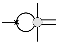
Figure 4: Coleman-Thun type singularity in the shift current Ward identity

This does not happen at one loop for the processes with different flavors that we consider though, because the shadowed part of the graph in Figure 4 vanishes as a consequence of integrability and absence of annihilations at the tree level.

4 Superstrings

Let us see now whether the no-go result presented above can be avoided in the presence of additional massless particles on the worldsheet. In this paper we restrict to the simplest possibility, namely when the additional particles are all goldstini—massless fermions arising as a consequence of non-linearly realized super-Poincaré symmetry. In addition to the bosonic fields $X^{i}$ we now have massless fermionic fields, $\theta^{A}$ which in what follows always belong to irreducible representations of the bulk Lorentz group. The Roman index $A$ runs from 1 to the total number of extended supersymmetries $\mathcal{N}$. Usually the absence of higher spin particles imposes an upper bound on $\mathcal{N}$, but from the point of view of non-linear realization any $\mathcal{N}$ is consistent.

Let us first consider the situation when all bulk supersymmetries are broken by the string. Then the infinitesimal SUSY transformations are given by

$$\delta\theta^{A}=\epsilon^{A},\;\;\;\;\;\;\;\;\delta X^{\mu}=i\ell_{s}^{2}\bar{\epsilon}^{A}\Gamma^{\mu}\theta^{A},$$ (33)

where $\Gamma^{\mu}$ are D-dimensional gamma matrices. Here we introduced

$$X^{\mu}=(\sigma^{\alpha},\ell_{s}X^{i})$$

so that SUSY transformations shift not only the fields, but also the worldsheet coordinates.

Generalizing the Nambu-Goto action to incorporate this symmetry and the new fermionic fields is done in [29] by promoting $\partial_{\alpha}X^{\mu}$ (which is trivially invariant under translations of the bosonic embedding coordinates) to

$$\Pi_{\alpha}^{\mu}\equiv\partial_{\alpha}X^{\mu}-i\ell_{s}^{2}\bar{\theta}^{A}\Gamma^{\mu}\partial_{\alpha}\theta^{A},$$

which is clearly invariant under super-translations as well. Thus the action becomes

$$S_{VA}=-\frac{1}{\ell_{s}^{2}}\int d^{2}\sigma\sqrt{-\mathrm{det}\Pi^{\mu}_{\alpha}\Pi_{\mu\beta}},$$ (34)

which is a generalization of the action first considered by Volkov and Akulov in [31, 32]. As first noticed by Green and Schwarz [10], an additional term can be added to the Volkov-Akulov lagrangian (34) at the same order in the derivative expansion for special values of $D$ and $\mathcal{N}$. This new term is SUSY invariant only up to a total derivative. Interpreting this theory as a non-linear sigma model parameterizing the coset supergroup $SISO(1,D-1)/SO(1,D-1)$, the origin of this term is the non-trivial Chevalley-Eilenberg cohomology of the corresponding Lie superalgebra [33, 34]. This term, which is analogous to the Wess-Zumino term of the pion lagrangian [35], can only be written for $\mathcal{N}=1$ or $2$ and $D=3,4,6$ and $10$ which will be referred to as “special” dimensions. It takes the following form

$$S_{WZ}=ic\int d^{2}\sigma\left(\epsilon^{\alpha\beta}\partial_{\alpha}X^{\mu}(\bar{\theta^{1}}\Gamma_{\mu}\partial_{\beta}\theta^{1}-\bar{\theta^{2}}\Gamma_{\mu}\partial_{\beta}\theta^{2})+i\ell_{s}^{2}\bar{\theta^{1}}\Gamma^{\mu}\theta^{1}\bar{\theta^{2}}\Gamma_{\mu}\theta^{2}\right).$$ (35)

The full action that we are going to study is then

$$S=S_{VA}+S_{WZ}\;.$$ (36)

Unlike for the pion Lagrangian, the corresponding coupling constant $c$ does not have to be quantized and can be arbitrary. The choice $c=\pm 1$ corresponds to the GS superstring, which enjoys a non-obvious fermonic gauge symmetry ($\varkappa$-symmetry). In many respects, this case is similar to the bosonic string. Namely, one can solve the theory exactly by using the light-cone gauge quantization. Using the same arguments as in [20], one finds that the resulting finite volume spectrum corresponds to integrable reflectionless scattering with $S$-matrix determined by the phase shift (22). Famously, this quantization is consistent with non-linearly realized Poincaré symmetry only at $D=10$ (critical superstrings) and $D=3$ [36] .

Here we first concentrate on the remaining “non-special” choices of dimensions, and $c\neq\pm 1$ superstring in special dimensions. Later we will discuss the relation to the GS superstring as well. The formulas below are presented for the $N=2$ superstring with a WZ term. To obtain the results for the $N=1$ superstring, one needs to set one of the spinors to zero. To obtain the results for non-special dimensions, one needs to set $c=0$.

Since the unbroken linearly realized symmetry subgroup is $SO(1,1)\times SO(D-2)$, the following representation of the gamma matrices is convenient

$$\Gamma^{\alpha} =\rho^{\alpha}\otimes\mathbb{1}$$

$$\Gamma^{j} =\rho^{*}\otimes\gamma^{j}\;,$$ (37)

where $\gamma^{j}$ are $(D-2)$-dimensional gamma matrices, and $\rho^{\alpha}$ are two dimensional gamma matrices, which will be chosen in the Weyl basis,

$$\rho^{0}=\left(\begin{array}[]{cc}0&-1\\ 1&0\end{array}\right),\;\rho^{1}=\left(\begin{array}[]{cc}0&1\\ 1&0\end{array}\right),\;\rho^{*}=\rho^{0}\rho^{1}.$$

4.1 The Quartic Vertex

We expand the Lagrangian in $\ell_{s}$ and canonically normalize the spinors as

$$\theta^{A}\rightarrow\left(\left(2(\mathbb{1}+(-)^{A}c\rho^{*})\right)^{-1/2}\otimes\mathbb{1}\right)\theta^{A}$$

to obtain

$$\mathcal{L}=-\tfrac{1}{2}\partial_{\alpha}X^{j}\partial^{\alpha}X_{j}+i\frac{1}{2}\bar{\theta}^{A}\not{\partial}\theta^{A}+i\ell_{s}\frac{\left(\eta^{\alpha\beta}+(-)^{A}c\epsilon^{\alpha\beta}\right)}{2\sqrt{1-c^{2}}}\left(\bar{\theta}^{A}\rho^{*}\gamma^{j}\partial_{\alpha}\theta^{A}\right)\partial_{\beta}X_{j}+\ldots$$ (38)

Since all cubic vertices vanish on-shell for any value of $c$ it is convenient to perform the following field redefinitions, which remove them altogether,

$$\theta^{A}\rightarrow \theta^{A}+\ell_{s}\lambda_{A}\partial_{\alpha}X^{i}\rho^{*}\rho^{\alpha}\otimes\gamma_{i}\theta^{A}$$

$$X^{i}\rightarrow X^{i}+\ell_{s}\eta_{A}\bar{\theta}^{A}\rho^{*}\otimes\gamma^{i}\theta^{A}\;.$$ (39)

Here $A$ runs from 1 to 2 and summation is implied for the bosonic field redefinition. Notice that $X^{i}$ shifts by a pseudoscalar quantity, because the Wess-Zumino contribution to the Lagrangian (35) is a pseudoscalar with respect to the worldsheet Lorentz group, $SO(1,1)$.

The coefficients of the field redefinitions that cancel the three point vertices of the lagrangian are universal (i.e., the same for every $D$) and take the form

$$\lambda_{A}= -\frac{1-(-)^{A}c}{\sqrt{1-c^{2}}}$$

$$\eta_{A}= \ \ \ (-)^{A}\frac{-c}{\sqrt{2-2c^{2}}}$$

First, we restrict our attention to the case of $\mathcal{N}=1$ and special dimensions. The results for the $2\to 2$ scattering are presented in Figure 5. Just like for a bosonic string, we find that the amplitude describes pure transmission. Moreover, the corresponding phase shift is independent of $c$ and the same for all processes (the relative minus sign for the fermions comes from the ordering of in and out states, that is for a free fermion the $S$-matrix would be $-1$). In other words, to the leading order the $S$-matrix is proportional to the identity operator and is given by (13), as before.

Let us now turn to the case of $\mathcal{N}=2$. Naturally, as long as the processes involving only $A=1$ or $A=2$ fermions are considered, all properties of $\mathcal{N}=1$ amplitudes remain. However, processes involving both types of fermions are present, and for them the $S$-matrix is no longer proportional to the identity. It exhibits both annihilations in the flavor $A$-space, and non-trivial structure in $SO(D-2)$ spinor space. Moreover, some of the amplitudes now depend on $c$, and become divergent at $c=\pm 1$. Several examples of amplitudes (with spinor structure suppressed) are presented on Figure 6.

$$\frac{1}{4E_{1}E_{2}}\cdot\left(\begin{array}[]{c}\includegraphics[height=62.59596pt]{2p2pdashed.pdf}\end{array}\right)= \frac{1}{2E_{2}}\cdot\left(\begin{array}[]{c}\includegraphics[height=62.59596pt]{2p2pdashed_solid.pdf}\end{array}\right)=-1\cdot\left(\begin{array}[]{c}\includegraphics[height=62.59596pt]{2p2p.pdf}\end{array}\right)=\frac{is\ell_{s}^{2}}{2}\ .$$

Figure 5: 4-point interactions between branons and goldstini. The solid line represents a goldstino corresponding to one broken supercharge. Time is flowing upwards (also in all later Figures). The amplitudes containing bosons need to be divided by the norm of the bosonic states to obtain the corresponding $S$-matrix element.

$$\begin{array}[]{c}\includegraphics[height=62.59596pt]{2p2pdouble_single.pdf}\end{array}=-i\frac{s\ell_{s}^{2}}{1+c}\ ,\begin{array}[]{c}\includegraphics[height=62.59596pt]{2p2psingle_double.pdf}\end{array}=-i\frac{s\ell_{s}^{2}}{1-c}\ ,\begin{array}[]{c}\includegraphics[height=62.59596pt]{2to2production.pdf}\end{array}=-i\frac{s\ell_{s}^{2}}{2}\ .$$

Figure 6: 4-point interactions among fermions corresponding to different broken supercharges, which are labeled by single and double lines.

4.2 The Quintic Vertex

From the previous experience with a bosonic string, one may expect that a non-trivial structure of the $2\to 2$ amplitudes indicates the breakdown of integrability for processes with a larger number of particles. To check this, let us inspect five-particle processes. This is rather straightforward because, after the field redefinition (4.1), only the quintic vertices in the Lagrangian contributes to this processes. One finds that the only quintic vertex which remains is the one with four fermions and one boson. For non-special number of dimensions it does not vanish on shell. The same is true for ${\cal N}=2$, $c\neq\pm 1$, for processes involving fermions of different flavors. This proves that superstrings are not integrable for these choices of the parameters. However, somewhat surprisingly, all quintic vertices vanish on shell for the ${\cal N}=1$ superstring in special dimensions, independently of the value of $c$. We will discuss the reason and implications of this cancellation in the next subsection. Before doing that, it is instructive to discuss in some more detail the structure of the quintic vertex when it does not vanish.

An example of a non-vanishing $\mathcal{N}=2$ quintic amplitude is shown in Figure 7, where $p_{-}$ is the momentum of one of the $A=2$ fermions, and we suppressed the spinor indices. Values $c=\pm 1$ are special again due to the emergence of $\kappa$-symmetry at these points.

$$\begin{array}[]{c}\includegraphics[height=62.59596pt]{5point.pdf}\end{array}=i\ell_{s}^{3}\sqrt{\frac{1+c}{1-c}}p_{+}p_{-}^{2}\ .$$

Figure 7: The 5-point vertex does not vanish for $\mathcal{N}=2$ away from $c=\pm 1$ for processes involving both $A=1$ (single line) and $A=2$ (double line) goldstini.

Even though all our fermions are goldstinos of spontaneously broken SUSY generators, the non-vanishing quintic amplitudes are not soft with respect to the momenta of some of the fermions. This implies that singular terms must be present in the SUSY Ward identities similarly to the bosonic case of section 3.1. These singularities, however, are not specific to 2 dimensions, rather they are analogous to the contributions present in the case of pion-nucleon scattering and related to the terms quadratic in fields present in the non-linear currents [17].

Indeed, after canonically normalizing the fields, the SUSY transformations (33) become

$$\delta_{\epsilon^{A}}\theta^{A^{\prime}} =\delta^{A^{\prime}}_{A}\left(\mathbb{1}+(-)^{A}c\rho^{*}\right)^{+1/2}\epsilon^{A}+i\ell_{s}\bar{\theta}^{A}\left(\mathbb{1}-(-)^{A}c\rho^{*}\right)^{-1/2}\rho^{\alpha}\epsilon^{A}\partial_{\alpha}\theta^{A^{\prime}}/2$$

$$\delta_{\epsilon^{A}}X^{j} =-i\bar{\theta}^{A}\left(\mathbb{1}-(-)^{A}c\rho^{*}\right)^{-1/2}\rho^{*}\gamma^{j}\epsilon^{A}/2+i\ell_{s}\bar{\theta}^{A}\left(\mathbb{1}-(-)^{A}c\rho^{*}\right)^{-1/2}\rho^{\alpha}\epsilon^{A}\partial_{\alpha}X^{j}/2\ ,$$ (40)

and the conserved fermionic current corresponding to this symmetry is

$$\mathcal{J}^{\alpha A}=\left(\mathbb{1}-(-)^{A}c\rho^{*}\right)^{1/2}\rho^{\alpha}\theta^{A}+\ell_{s}\left(\mathbb{1}+(-)^{A}c\rho^{*}\right)^{-1/2}\rho^{*}\gamma^{j}\theta^{A}\left(\eta^{\alpha\beta}-(-)^{A}c\epsilon^{\alpha\beta}\right)\partial_{\beta}X_{j}+\ldots\ ,$$ (41)

which gives the following Ward identity

$$\not{\partial}\left\langle out|\theta^{A}|in\right\rangle=-\frac{\eta^{\alpha\beta}-(-)^{A}c\epsilon^{\alpha\beta}}{\sqrt{1-c^{2}}}\ell_{s}\left\langle out|\rho^{*}\gamma^{j}\partial_{\alpha}\left(\theta^{A}\partial_{\beta}X_{j}\right)|in\right\rangle+\ldots\ .$$ (42)

To see how this formula works in detail, we will consider a particular example in $\mathcal{N}=2$, $D=4$. In the basis (37) the Majorana fermion can be parametrized as

$$\Theta^{A}=\left(\left(\begin{array}[]{c}\alpha_{A}\\ \alpha_{A}^{\dagger}\end{array}\right),\left(\begin{array}[]{c}\beta_{A}\\ \beta_{A}^{\dagger}\end{array}\right)\right)$$ (43)

where the $\alpha$’s are right-moving and $\beta$’s are left-moving, and both have positive $SO(2)$ helicities. In this notation the kinetic term reads

$$-i\sqrt{2}\alpha_{A}\partial_{+}\alpha_{A}^{\dagger}-i\sqrt{2}\beta_{A}\partial_{-}\beta^{\dagger}_{A}\;.$$ (44)

Since the quintic vertex that we consider has three derivatives, the worldsheet Lorentz invariance requires that the process involving, say, a left-moving boson always has one left-moving and three right-moving fermions.

First, let us consider a process where all fermions are of the same flavor and demonstrate that it has a vanishing amplitude as a consequence of Ward identities. To be specific, let us take the following initial and final states:

$$\alpha_{1}(p_{-})\beta_{1}(p_{+})\rightarrow\alpha_{1}^{\dagger}(k_{-})\alpha_{1}(p_{-}\!-k_{-})X(p_{+})\ .$$ (45)

The only vertex that can contribute to this amplitude is

$$\partial_{-}\alpha_{1}\alpha_{1}\alpha_{1}^{\dagger}\partial_{+}\beta\partial_{+}X^{\dagger}\;.$$ (46)

The corresponding amplitude is not soft with respect to both $k_{-}$ and $q_{-}=p_{-}\!-k_{-}$. Let us check whether this is consistent with the Ward identity (42) applied to the process (45) in the limit $k_{-}\to 0$. The diagrams that can develop a singularity are shown in Figure 8.

$$\begin{array}[]{c}\includegraphics[height=62.59596pt]{5pointward.pdf}\end{array}=\begin{array}[]{c}\includegraphics[height=62.59596pt]{Wardferm2.pdf}\end{array}+\begin{array}[]{c}\includegraphics[height=62.59596pt]{Wardferm1.pdf}\end{array}+\ldots$$

Figure 8: Singular diagrams in Ward identities for a 5-particle process involving one branon and goldstini of one supercharge. Arrows show the flow of the $SO(2)$ helicity.

In the soft limit, the internal propagators of both diagrams go on shell, and the matrix element factorizes into the product of the 4-point amplitude, the propagator, and the matrix element of the operator in the right hand side of (42) between a boson and a fermion analogously to (32). Since we found that the corresponding $S$-matrices are equal in magnitudes but have opposite signs (see Figure 5) the sum of these two diagrams vanish. We conclude then that the vertex (46) should vanish, in agreement with what we found by a brute force calculation.

On the other hand, let us consider the process

$$\alpha_{1}(p_{-})\beta_{1}(p_{+})\rightarrow\alpha_{2}^{\dagger}(k_{-})\alpha_{2}(q_{-})X^{\dagger}(p_{+})\ .$$ (47)

As a result of our field redefinition, there is a single vertex which contributes to this process, which is

$$\ell_{s}^{3}\sqrt{\frac{1+c}{1-c}}\partial_{-}\alpha_{2}^{\dagger}\alpha_{2}\alpha_{1}\partial_{+}\beta_{1}\partial_{+}X^{\dagger}\ ,$$ (48)

and the corresponding amplitude is

$$\mathcal{M}_{(5)}=i\ell_{s}^{3}\sqrt{\frac{1+c}{1-c}}q_{-}p_{+}^{2}\;,$$ (49)

which is not soft with respect to $k_{-}$. To see whether this behavior is consistent with the Ward identities we again inspect the right-hand side of (42) in the limit $k_{-}\rightarrow 0$. This time there is only one singular contribution as shown in Figure 9,

$$\begin{array}[]{c}\includegraphics[height=62.59596pt]{5pointwardN2.pdf}\end{array} =\begin{array}[]{c}\includegraphics[height=62.59596pt]{Wardferm1N2.pdf}\end{array}+\ldots$$

Figure 9: Singular diagram in Ward identities for a 5-particle process involving one boson and two different flavors of fermions.

$$\mathcal{M}_{(5)}=k_{-}\left(-p_{+}\frac{1+c}{\sqrt{1-c^{2}}}\ell_{s}\right)\frac{-i}{k_{-}}i\mathcal{M}_{(4)}\left(s\right)+O(k_{-})$$ (50)

where $s=2p_{-}p_{+}$ and $\mathcal{M}_{(4)}$ is the third amplitude in Figure 6. This illustrates that the Ward identities indeed fix the quintic amplitude.

Note that $\mathcal{M}_{(5)}$ is soft with respect to $q_{-}$. It also follows immediately from the Ward identity argument since the singular contribution in the $q_{-}\to 0$ limit would require the $\alpha_{1}\beta_{1}\to\alpha_{2}^{\dagger}\beta_{2}^{\dagger}$ part of $\mathcal{M}_{(4)}$ which is zero due to $SO(2)$ helicity conservation.

To summarize this section, we see that in addition to the conventional GS superstring, only $\mathcal{N}=1$ theories in $D=3,4,6,10$ with arbitrary value of $c$ stay as viable candidates to be integrable. Let us take now a closer look at this remaining set of models.

4.3 $\mathcal{N}=1$: A Closer Look

Interestingly, all $\mathcal{N}=1$, $D=3,4,6,10$ amplitudes, which we calculated so far, are independent of the Wess–Zumino coupling constant $c$. Furthermore, the set of physical degrees of freedom in these theories is equivalent to the $\mathcal{N}=2$ Green-Schwarz superstring after all gauge degrees of freedom are removed. This suggests that these models are all equivalent to $\mathcal{N}=2$ GS superstrings at the same number of dimensions. In fact, this observation has already been made for $c=0$ [37] (see also [38] for a detailed analysis of the $D=3$, $c=0$ case). In this case, one can start with $\mathcal{N}=2$ GS superstring and fix the $\varkappa$-symmetry, by imposing the condition $\theta^{1}=\theta^{2}$. The resulting action is $\mathcal{N}=1$, $c=0$ superstring, which proves the equivalence at $c=0$. To extend the prove for all values of $c\neq\pm 1$ we will show now that the WZ term can be removed by a field redefinition, and hence the theories are indeed equivalent for all values of $c$.

To do this, we need to look in some detail at the full classical field equations for $\mathcal{N}=1$ theory. For this purpose it is convenient to introduce $X^{0}$ and $X^{1}$ as dynamical fields and rewrite the action in the Polyakov form

$$S=\int d^{2}\sigma\left(-\frac{1}{2}\sqrt{-h}h^{\alpha\beta}\Pi^{\mu}_{\alpha}\Pi_{\beta\mu}-ic\epsilon^{\alpha\beta}\bar{\theta}\hat{\Pi}_{\alpha}\partial_{\beta}\theta\right)$$ (51)

where $\ell_{s}$ is set to unity since it is no longer needed as an expansion parameter and $\hat{\Pi}_{\alpha}\equiv\Gamma_{\mu}\Pi^{\mu}_{\alpha}$. Here $\theta$ satisfies the following identities

$$\bar{\theta}_{1}\Gamma^{\mu}\theta_{2}=-\bar{\theta}_{2}\Gamma^{\mu}\theta_{1}$$ (52)

$$\Gamma^{\mu}\theta_{[1}\bar{\theta}_{2}\Gamma_{\mu}\theta_{3]}=0\;,$$ (53)

which are specific to the GS choices of $D$ and $\theta$-representations, and ensure that the WZ term is invariant under SUSY transformations. At $c\not=\pm 1$ this action has no local fermonic symmetry and explicitly has only $\mathcal{N}=1$ supersymmetry.

Let us show now that for any $c\neq\pm 1$ the WZ term in the action vanishes on shell (i.e., as a consequence of the exact field equations). This will imply, that the parameter $c\neq\pm 1$ can indeed be changed arbitrarily by a field redefinition and that this whole one parameter family of theories is equivalent to the $\mathcal{N}=2$ Green-Schwarz action at $c=\pm 1$.

The variation of the action with respect to the auxiliary metric yields the following constraints

$$T_{\alpha\beta}\equiv-\frac{2}{\sqrt{-h}}\frac{\delta S}{\delta h^{\alpha\beta}}=\Pi^{\mu}_{\alpha}\Pi_{\beta\mu}-\frac{1}{2}h_{\alpha\beta}h^{\gamma\delta}\Pi^{\mu}_{\gamma}\Pi_{\delta\mu}.$$ (54)

Note that as a consequence of Weyl invariance the energy momentum tensor is traceless.

The Euler–Lagrange equations for scalars and fermions are

$$\frac{\delta S}{\delta X^{\mu}}=\partial_{\alpha}\left(\sqrt{-h}h^{\alpha\beta}\Pi_{\beta\mu}+ic\epsilon^{\alpha\beta}\bar{\theta}\Gamma_{\mu}\partial_{\beta}\theta\right)=0$$ (55)

$$\frac{1}{2}\frac{\delta S}{\delta\bar{\theta}}=i(\sqrt{-h}h^{\alpha\beta}-c\epsilon^{\alpha\beta})\hat{\Pi}_{\alpha}\partial_{\beta}\theta+\frac{i}{2}\partial_{\alpha}\left(\sqrt{-h}h^{\alpha\beta}\hat{\Pi}_{\beta}\right)\theta+c\epsilon^{\alpha\beta}\Gamma^{\mu}\partial_{\beta}\theta\bar{\theta}\Gamma_{\mu}\partial_{\alpha}\theta=0.$$ (56)

The Fierz identities (52) and (53) imply

$$\epsilon^{\alpha\beta}\Gamma^{\mu}\partial_{\beta}\theta(\bar{\theta}\Gamma_{\mu}\partial_{\alpha}\theta)=-\frac{1}{2}\epsilon^{\alpha\beta}\Gamma^{\mu}\theta(\partial_{\alpha}\bar{\theta}\Gamma_{\mu}\partial_{\beta}\theta),$$

which allows one to show that the last two terms of (56) vanish due to the scalar field equations (55). To further simplify the field equations, we choose the orthogonal gauge

$$h^{\alpha\beta}\sim\eta^{\alpha\beta}=\left(\begin{array}[]{cc}0&1\\ 1&0\end{array}\right).$$

In this gauge, labeling the coordinates as $``+"$ and $``-"$, the field equations become

$$\Pi_{+}^{2}=\Pi_{-}^{2}=0$$ (57)

$$(1+c)\partial_{-}\Pi_{+}+(1-c)\partial_{+}\Pi_{-}=0$$ (58)

$$(1+c)\hat{\Pi}_{-}\partial_{+}\theta+(1-c)\hat{\Pi}_{+}\partial_{-}\theta=0.$$ (59)

Note that as a consequence of (57) the operators

$$\hat{\Pi}_{\pm}\equiv\Gamma^{\mu}\Pi_{\mu\pm},$$

are nilpotent, $\hat{\Pi}^{2}_{\pm}=0$. Then from (59) it follows that

$$\hat{\Pi}_{+}\hat{\Pi}_{-}\partial_{+}\theta=\hat{\Pi}_{-}\hat{\Pi}_{+}\partial_{-}\theta=0\;.$$ (60)

We will restrict ourselves to configurations in which the operator $\hat{P}\equiv\hat{\Pi}_{-}+\hat{\Pi}_{+}$ has no null vectors. Then (60) implies that

$$\hat{P}(\hat{\Pi}_{-}\partial_{+}\theta)=\hat{P}(\hat{\Pi}_{+}\partial_{-}\theta)=0,$$

hence

$$\hat{\Pi}_{-}\partial_{+}\theta=\hat{\Pi}_{+}\partial_{-}\theta=0,$$ (61)

on the equations of motion for any $c\neq\pm 1$. This implies that the WZ action, which can be written as

$$S_{WZ}=ic\int d^{2}\sigma(\bar{\theta}\hat{\Pi}_{+}\partial_{-}\theta-\bar{\theta}\hat{\Pi}_{-}\partial_{+}\theta),$$

vanishes as a consequence of field equations for all $c\neq\pm 1$, so that this term can be removed by a field redefinition and theories with different values of $c$ are equivalent. At the end of the next section we will present an explicit form for the corresponding infinitesimal field redefinition connecting different values of $c$.

4.4 Hidden Symmetry

The arguments above explain why $c\neq\pm 1$, $\mathcal{N}=1$ theories are all equivalent to $\mathcal{N}=2$ GS superstrings. This equivalence implies that $\mathcal{N}=1$ theories should have an additional hidden supersymmetry, corresponding to the second supercharge of the $\mathcal{N}=2$ GS theory. This supersymmetry should be realized linearly. Given that $\mathcal{N}=1$ theories have enhanced infinite dimensional fermionic symmetries at $c=\pm 1$ ($\varkappa$-symmetries), to identify the hidden symmetry it is natural to inspect whether any combination of $\varkappa$-symmetry transformations survives at $c\neq\pm 1$ as well. The most general combination of two infinitesimal $\varkappa$-symmetry transformations can be written as

$$\delta\theta=\hat{\Pi}_{\alpha}(e^{\alpha}_{-}\kappa_{+}+e^{\alpha}_{+}\kappa_{-})$$

$$\delta X^{\mu}=i\bar{\theta}\Gamma^{\mu}\delta\theta$$

$$\delta\Pi^{\mu}_{\alpha}=2i\partial_{\alpha}\bar{\theta}\Gamma^{\mu}\delta\theta$$

$$\delta e^{\alpha}_{+}=4ie^{\alpha}_{-}e^{\beta}_{+}\bar{\kappa}_{-}\partial_{\beta}\theta$$

$$\delta e^{\alpha}_{-}=4ie^{\alpha}_{+}e^{\beta}_{-}\bar{\kappa}_{+}\partial_{\beta}\theta$$

$$\delta\left(\sqrt{-h}h^{\alpha\beta}\right)=8i\sqrt{-h}(e^{\alpha}_{-}e^{\gamma}_{+}e^{\beta}_{-}\bar{\kappa}_{+}+e^{\alpha}_{+}e^{\gamma}_{-}e^{\beta}_{+}\bar{\kappa}_{-})\partial_{\gamma}\theta\;,$$ (62)

where we introduced the “zweibein” fields, $e_{\pm}^{\alpha}$, such that $h^{\alpha\beta}=e_{+}^{\alpha}e_{-}^{\beta}+e_{+}^{\beta}e_{-}^{\alpha}$. One can check that these transformations leave the action invariant when one picks $c=\pm 1,\kappa_{\mp}=0$ and arbitrary $\kappa_{\pm}$. For a general $c$, the action variation under a general combination of $\kappa$-transformations takes the following form

$$\delta S=-2i\int d^{2}\sigma\epsilon^{\alpha\beta}\partial_{\alpha}\bar{\theta}\hat{\Pi}_{\beta}\left((c-1)\hat{\Pi}_{-}\kappa_{+}+(c+1)\hat{\Pi}_{+}\kappa_{-}\right),$$ (63)

where operators $\hat{\Pi}_{\pm}\equiv\hat{\Pi}_{\alpha}e^{\alpha}_{\pm}$ coincide in the conformal gauge with $\hat{\Pi}_{\pm}$ used in the previous section. For this variation to be zero, we need to chose spinors $\kappa_{\pm}$ in such a way that

$$(c-1)\hat{\Pi}_{-}\kappa_{+}+(c+1)\hat{\Pi}_{+}\kappa_{-}=0.$$ (64)

For a generic off-shell configuration $\hat{\Pi}_{\pm}$ are non-degenerate, so one can use (64) to express $\kappa_{+}$ through $\kappa_{-}$ and naively one is left with a local symmetry for any $c$. However, for all on-shell configurations $\hat{\Pi}_{\pm}$ are nilpotent and the only way to solve (64) is to set separetly

$$\hat{\Pi}_{-}\kappa_{+}=\hat{\Pi}_{+}\kappa_{-}=0.$$ (65)

Unfortunately, transformations of this form act trivially on-shell and do not lead to any interesting symmetry. The way out is to note the following consequence of the Fierz identities (57) and (58),

$$\epsilon^{\alpha\beta}\Gamma^{\mu}\theta(\partial_{\alpha}\bar{\theta}\Gamma_{\mu}\partial_{\beta}\theta)=\frac{2}{3}\epsilon^{\alpha\beta}\partial_{\alpha}(\Gamma^{\mu}\theta(\bar{\theta}\Gamma_{\mu}\partial_{\beta}\theta)),$$

implying that $\epsilon^{\alpha\beta}\partial_{\alpha}\bar{\theta}\hat{\Pi}_{\beta}$ is a total derivative,

$$\epsilon^{\alpha\beta}\partial_{\alpha}\bar{\theta}\hat{\Pi}_{\beta}=\epsilon^{\alpha\beta}\partial_{\alpha}\left(\bar{\theta}\Gamma_{\mu}\left(\partial_{\beta}X^{\mu}-\frac{i}{3}\bar{\theta}\Gamma^{\mu}\partial_{\beta}\theta\right)\right).$$

This means that we can integrate (63) by parts and the variation of the action will vanish under a weaker condition, as compared to (64),

$$(c-1)\hat{\Pi}_{-}\kappa_{+}+(c+1)\hat{\Pi}_{+}\kappa_{-}=const.$$

This weaker condition allows us to solve for a new non-trivial symmetry of the action, namely

$$\kappa_{\pm}=\frac{\hat{\Pi}_{\pm}}{2(c\mp 1)\Pi^{\mu}_{+}\Pi_{-\mu}}\kappa,$$ (66)

where $\kappa$ is a constant spinor. On a long string background this generator is spontaneously broken. However, one can choose a linear combination of the hidden SUSY transformation and of the conventional one (33) which is realized linearly.

To complete the discussion of this new symmetry, we derive the associated conserved Nöether current via the usual prescription. Take the parameter of the transformation $\kappa$ to be an arbitrary function on the worldsheet. Then the variation of the action (51) takes the following form

$$\delta S=-2i\int d^{2}\sigma\epsilon^{\alpha\beta}\partial_{\alpha}\bar{\kappa}\left(\partial_{\beta}X^{\mu}-\frac{i}{3}\bar{\theta}\Gamma^{\mu}\partial_{\beta}\theta\right)\Gamma_{\mu}\theta,$$

which yields the supercurrent

$$j^{\alpha}_{\kappa}=2i\frac{\epsilon^{\alpha\beta}}{\sqrt{-h}}\left(\partial_{\beta}X^{\mu}-\frac{i}{3}\bar{\theta}\Gamma^{\mu}\partial_{\beta}\theta\right)\Gamma_{\mu}\theta.$$

On the other hand, the conventional supercurrent corresponding to transformations (33) is

$$j^{\alpha}_{\epsilon}=2ih^{\alpha\beta}\hat{\Pi}_{\beta}\theta+2ic\frac{\epsilon^{\alpha\beta}}{\sqrt{-h}}\left(\partial_{\beta}X^{\mu}+\frac{i}{3}\bar{\theta}\Gamma^{\mu}\partial_{\beta}\theta\right)\Gamma_{\mu}\theta.$$

The existence of a hidden linearly realized SUSY confirms the equivalence of the model to the standard $\mathcal{N}=2$ GS supersting. Since both currents have the same chirality our construction corresponds to the chiral IIB theory.

Finally, to present the field redefinition, which shifts the coefficient of the WZ term in the action, let us modify the hidden symmetry (66) to

$$\kappa_{\pm}=\epsilon\frac{\hat{\Pi}_{\pm}}{4(c\mp 1)\Pi^{\mu}_{+}\Pi_{-\mu}}\theta,$$ (67)

where $\epsilon$ is some infinitesimal c-number. When these choices are made for the infinitesimal spinors in a general $\kappa$ transformation (62), from (63) it is straightforward to demonstrate that

$$\delta_{\epsilon}S=i\epsilon\int(\bar{\theta}\hat{\Pi}_{+}\partial_{-}\theta-\bar{\theta}\hat{\Pi}_{-}\partial_{+}\theta)=\epsilon S_{WZ},$$ (68)

which is exactly what required for a field redefinition which changes the value of $c$.

5 Conclusions

To summarize, we feel that the presented analysis elucidates the relation between integrability on the fluxtube worldsheet and the conventional condition for the string to be critical. As our results show, if the only gapless degrees of freedom on the flux tube are Goldstones and Goldstini of spontaneously broken flat space-time (super)symmetries, then in addition to conventional critical strings, the only other case when the worldsheet theory may be integrable is $D=3$. It will be interesting to understand whether these $D=3$ theories (which were studied recently in [25, 39]) may be obtained from a consistent interacting bulk theory. One puzzle related to them is that $D=3$ case does not appear special neither in the Polchinski–Strominger description, nor in the conventional Liouville approach to non-critical strings.

Coming back to the initial question which motivated our analysis, namely the search for integrable confining strings in four dimensional large $N$ gauge theories, we see that theories of this kind necessarily need to carry additional gapless degrees of freedom. Of course, this still leaves a room for many interesting possibilities. It appears likely that answering this question will require using more sophisticated field/string theory tools. The approach of this paper, based on universality of worldsheet scattering at (several) leading orders in the derivative expansion, will hopefully serve as a useful cross-check and/or guideline in this search.

For example, the integrability condition can be satisfied by adding massless fermions, which are not related to spontaneously broken supersymmetry. We checked, for instance, the behavior of the one-loop bosonic $2\to 2$ amplitude in the presence of $N$ worldsheet Dirac (or $4N$ Majorana-Weyl) fermions, that trivially transform under $SO(D-2)$. The result is equal to (14) with $(D-26)$ replaced with $(D+2N-26)$. This gives the same counting as in the case of the heterotic string where one fermionic degree of freedom contributes to the central charge as half of a boson.

6 Acknowledgements

We would like to thank Nima Arkani-Hamed, Raphael Flauger, Matthew Kleban, Mehrdad Mirbabayi, Arkady Tseytlin and Luke Underwood for useful discussions. This work is supported in part by the NSF under grants PHY-1068438 and PHY-1316452, and by the NSF CAREER award PHY-1352119. The work of SS was supported in part by Fondazione Angelo della Riccia.

7 Appendix: Scalar Triangle

After the numerators of triangle diagrams are reduced by the usual procedure we are left with the scalar triangle integral:

$$I_{3}=\int\frac{d^{d}q}{(2\pi)^{d}}\frac{1}{q^{2}(q+p_{1})^{2}(q+p_{1}+p_{2})^{2}}\;.$$ (69)

It was computed in arbitrary dimension in [40],

$$I_{3}=\frac{i}{2}(4\pi)^{-\frac{d}{2}}\frac{r}{(2-d/2)}\alpha_{1}\alpha_{2}\alpha_{3}\Delta^{\frac{3-d}{2}}\left(f(\delta_{1})+f(\delta_{2})+f(\delta_{3})+c\right),$$ (70)

where the following notations are introduced

$$s_{ij}=(p_{i}+p_{j})^{2},\quad p_{3}=-p_{1}-p_{2},\quad s_{12}=\frac{-1}{\alpha_{1}\alpha_{3}},\quad s_{23}=\frac{-1}{\alpha_{1}\alpha_{2}},\quad s_{31}=\frac{-1}{\alpha_{2}\alpha_{3}}\;,$$ (71)

$$\gamma_{i}=\sum_{j=1,3}\alpha_{j}-2\alpha_{i}\;,$$ (72)

$$\Delta=\sum_{i>j}\gamma_{i}\gamma_{j}\;,$$ (73)

$$\delta_{i}=\gamma_{i}/\sqrt{\Delta}\;,$$ (74)

$$f(\delta)=4^{\frac{d}{2}-1}\delta_{\,2}F_{1}\left(\frac{d}{2}-1,\frac{1}{2};\frac{3}{2};-\delta^{2}\right)\;,$$ (75)

$$c=-2\pi\frac{\Gamma(d-3)}{\Gamma\left(\frac{d}{2}-1\right)^{2}}\;,$$ (76)

$$r=\frac{\Gamma\left(3-\frac{d}{2}\right)\Gamma\left(\frac{d}{2}-1\right)^{2}}{\Gamma\left(d-3\right)}.$$ (77)

Since (70) has a pole at $d=2$ we need to know the taylor expansion of the hypergeometric function with respect to its first parameter. In our case it takes the following simple form [41],

$${}_{2}F_{1}(\epsilon,\frac{1}{2};\frac{3}{2};z)=1+\epsilon\left(-2\frac{\operatorname{arctanh}\sqrt{z}}{\sqrt{z}}-\log(1-z)+2\right)+O(\epsilon^{2})\;.$$ (78)

References

- [1] G. Veneziano, “Construction of a crossing - symmetric, Regge behaved amplitude for linearly rising trajectories,” Nuovo Cim. A57 (1968) 190–197.
- [2] M. Shifman and A. Vainshtein, “Highly Excited Mesons, Linear Regge Trajectories and the Pattern of the Chiral Symmetry Realization,” Phys.Rev. D77 (2008) 034002, 0710.0863.
- [3] N. Beisert, C. Ahn, L. F. Alday, Z. Bajnok, J. M. Drummond, et al., “Review of AdS/CFT Integrability: An Overview,” Lett.Math.Phys. 99 (2012) 3–32, 1012.3982.
- [4] N. Gromov, V. Kazakov, S. Leurent, and D. Volin, “Quantum spectral curve for arbitrary state/operator in AdS5/CFT4,” 1405.4857.
- [5] S. Dubovsky, R. Flauger, and V. Gorbenko, “Evidence from Lattice Data for a New Particle on the Worldsheet of the QCD Flux Tube,” Phys.Rev.Lett. 111 (2013), no. 6, 062006, 1301.2325.
- [6] S. Dubovsky, R. Flauger, and V. Gorbenko, “Flux Tube Spectra from Approximate Integrability at Low Energies,” 1404.0037.
- [7] A. Athenodorou, B. Bringoltz, and M. Teper, “Closed flux tubes and their string description in D=3+1 SU(N) gauge theories,” JHEP 1102 (2011) 030, 1007.4720.
- [8] A. Athenodorou and M. Teper, “Closed flux tubes in higher representations and their string description in gauge theories,” JHEP 1306 (2013) 053, 1303.5946.
- [9] S. Dubovsky, R. Flauger, and V. Gorbenko, “Effective String Theory Revisited,” JHEP 1209 (2012) 044, 1203.1054.
- [10] M. B. Green and J. H. Schwarz, “Covariant Description of Superstrings,” Phys.Lett. B136 (1984) 367–370.
- [11] W. Siegel, “Hidden Local Supersymmetry in the Supersymmetric Particle Action,” Phys.Lett. B128 (1983) 397.
- [12] L. Mezincescu, A. J. Routh, and P. K. Townsend, “All Superparticles are BPS,” J.Phys. A47 (2014) 175401, 1401.5116.
- [13] C. G. J. Callan, S. R. Coleman, J. Wess, and B. Zumino, “Structure of phenomenological Lagrangians. 2.,” Phys.Rev. 177 (1969) 2247–2250.
- [14] C. Isham, A. Salam, and J. Strathdee, “Nonlinear realizations of space-time symmetries. Scalar and tensor gravity,” Annals Phys. 62 (1971) 98–119.
- [15] D. V. Volkov, “Phenomenological Lagrangians,” Fiz.Elem.Chast.Atom.Yadra 4 (1973) 3–41.
- [16] E. Ivanov and V. Ogievetsky, “The Inverse Higgs Phenomenon in Nonlinear Realizations,” Teor.Mat.Fiz. 25 (1975) 164–177.
- [17] M. Bando, T. Kugo, and K. Yamawaki, “Nonlinear Realization and Hidden Local Symmetries,” Phys.Rept. 164 (1988) 217–314.
- [18] N. Arkani-Hamed, F. Cachazo, and J. Kaplan, “What is the Simplest Quantum Field Theory?,” JHEP 1009 (2010) 016, 0808.1446.
- [19] D. Kapec, V. Lysov, S. Pasterski, and A. Strominger, “Semiclassical Virasoro symmetry of the quantum gravity -matrix,” JHEP 1408 (2014) 058, 1406.3312.
- [20] S. Dubovsky, R. Flauger, and V. Gorbenko, “Solving the Simplest Theory of Quantum Gravity,” JHEP 1209 (2012) 133, 1205.6805.
- [21] J. Polchinski and A. Strominger, “Effective string theory,” Phys.Rev.Lett. 67 (1991) 1681–1684.
- [22] P. Dorey, “Exact S matrices,” hep-th/9810026.
- [23] A. B. Zamolodchikov and A. B. Zamolodchikov, “Factorized s Matrices in Two-Dimensions as the Exact Solutions of Certain Relativistic Quantum Field Models,” Annals Phys. 120 (1979) 253–291.
- [24] P. Goddard, J. Goldstone, C. Rebbi, and C. B. Thorn, “Quantum dynamics of a massless relativistic string,” Nucl.Phys. B56 (1973) 109–135.
- [25] L. Mezincescu and P. K. Townsend, “Anyons from Strings,” Phys.Rev.Lett. 105 (2010) 191601, 1008.2334.
- [26] S. R. Coleman, “There are no Goldstone bosons in two-dimensions,” Commun.Math.Phys. 31 (1973) 259–264.
- [27] S. Weinberg, “Current-commutator theory of multiple pion production,” Phys. Rev. Lett. 16 (May, 1966) 879–883.
- [28] S. R. Coleman and H. Thun, “On the Prosaic Origin of the Double Poles in the Sine-Gordon S Matrix,” Commun.Math.Phys. 61 (1978) 31.
- [29] J. Hughes and J. Polchinski, “Partially Broken Global Supersymmetry and the Superstring,” Nucl.Phys. B278 (1986) 147.
- [30] E. Ivanov and S. Krivonos, “N=1 D = 4 supermembrane in the coset approach,” Phys.Lett. B453 (1999) 237–244, hep-th/9901003.
- [31] D. Volkov and V. Akulov, “Possible universal neutrino interaction,” JETP Lett. 16 (1972) 438–440.
- [32] D. Volkov and V. Akulov, “Is the Neutrino a Goldstone Particle?,” Phys.Lett. B46 (1973) 109–110.
- [33] J. M. Rabin, “Supermanifold Cohomology and the Wess-Zumino Term of the Covariant Superstring Action,” Commun.Math.Phys. 108 (1987) 375.
- [34] M. Henneaux and L. Mezincescu, “A Sigma Model Interpretation of Green-Schwarz Covariant Superstring Action,” Phys.Lett. B152 (1985) 340.
- [35] J. Wess and B. Zumino, “Consequences of anomalous Ward identities,” Phys.Lett. B37 (1971) 95.
- [36] L. Mezincescu, A. J. Routh, and P. K. Townsend, “Equivalence of 3D Spinning String and Superstring,” JHEP 1307 (2013) 024, 1305.5049.
- [37] A. R. Kavalov and A. G. Sedrakyan, “Quantum geometry of the covariant superstring with N = 1 global supersymmetry,” Physics Letters B 182 (Dec., 1986) 33–36.
- [38] W. Siegel, “Light Cone Analysis of Covariant Superstring,” Nucl.Phys. B236 (1984) 311.
- [39] L. Mezincescu and P. K. Townsend, “Quantum 3D Superstrings,” Phys.Rev. D84 (2011) 106006, 1106.1374.
- [40] Z. Bern, L. J. Dixon, and D. A. Kosower, “Dimensionally regulated pentagon integrals,” Nucl.Phys. B412 (1994) 751–816, hep-ph/9306240.
- [41] L. Ancarani and G. Gasaneo, “Derivatives of any order of the Gaussian hypergeometric function (2)F1(a, b, c z) with respect to the parameters a, b and c,” J.Phys. A42 (2009) 395208.