Chaotic Dynamics of Stellar Spin Driven by Planets Undergoing Lidov-Kozai Oscillations: Resonances and Origin of Chaos

Abstract

Many exoplanetary systems containing hot Jupiters are found to possess significant misalignment between the spin axis of the host star and the planet’s orbital angular momentum axis. A possible channel for producing such misaligned hot Jupiters involves Lidov-Kozai oscillations of the planet’s orbital eccentricity and inclination driven by a distant binary companion. In a recent work (Storch, Anderson & Lai 2014), we have shown that a proto-hot Jupiter undergoing Lidov-Kozai oscillations can induce complex, and often chaotic, evolution of the spin axis of its host star. Here we explore the origin of the chaotic spin behavior and its various features in an idealized non-dissipative system where the secular oscillations of the planet’s orbit are strictly periodic. Using Hamiltonian perturbation theory, we identify a set of secular spin-orbit resonances in the system, and show that overlaps of these resonances are responsible for the onset of wide-spread chaos in the evolution of stellar spin axis. The degree of chaos in the system depends on the adiabaticity parameter $\epsilon$, proportional to the ratio of the Lidov-Kozai nodal precession rate and the stellar spin precession rate, and thus depends on the planet mass, semi-major axis and the stellar rotation rate. For systems with zero initial spin-orbit misalignment, our theory explains the occurrence (as a function of $\epsilon$) of “periodic islands” in the middle of a “chaotic ocean” of spin evolution, and the occurrence of restricted chaos in middle of regular/periodic spin evolution. Finally, we discuss a novel “adiabatic resonance advection” phenomenon, in which the spin-orbit misalignment, trapped in a resonance, gradually evolves as the adiabaticity parameter slowly changes. This phenomenon can occur for certain parameter regimes when tidal decay of the planetary orbit is included.

1 Introduction

A major surprise in exoplanetary astrophysics in recent years is the discovery of the misalignment between the orbital axis of the planet and the spin axis of the host star in systems containing “hot Jupiters”, giant planets with orbital periods $\mathrel{\raise 1.29167pt\hbox{$<$}\mkern-14.0mu\lower 2.58334pt\hbox{$\sim$}}5$ days (e.g. Hebrard et al. 2008, Narita et al. 2009, Winn et al. 2009, Triaud et al. 2010, Hebrard et al. 2010, Albrecht et al. 2012). These planets cannot form in-situ, and must have migrated from a few AU’s distance from their host star to their current locations. Planet migration in protoplanetary disks is usually expected to produce aligned orbital and spin axes (however, see Bate, Lodato & Pringle 2010; Lai, Foucart & Lin 2011; Batygin 2012; Batygin & Adams 2013; Lai 2014; Spalding & Batygin 2014). So the observed misalignments suggest that dynamical interaction between planets and/or companion star may play an important role in the planet’s inward migration.

One of the dynamical channels for the migration of giant planets involves Lidov-Kozai oscillations (Lidov 1962; Kozai 1962) of the planet’s orbit induced by a distant companion (star or planet). When the companion’s orbit is sufficiently inclined relative to the planetary orbit, the planet’s eccentricity undergoes excursions to large values while the orbital axis precesses with varying inclination. Tidal dissipation in the planet at periastron reduces the orbital energy, leading to inward migration and circularization of the planet’s orbit (Wu & Murray 2003; Fabrycky & Tremaine 2007; Correia et al. 2011; Naoz et al. 2012; Petrovich 2014). A number of recent works have focused on the extreme evolution of the planetary orbit (such as orbital flip) when the octupole perturbing potential from the binary companion is included (Katz, Dong & Malhotra 2011; Naoz et al. 2011, 2013; Petrovich 2014; see also Ford et al. 2000; Li et al. 2014; Liu, Munoz & Lai 2014).

In a recent paper (Storch, Anderson & Lai 2014; hereafter SAL), we have shown that during the Lidov-Kozai cycle, gravitational interaction between the planet and its oblate host star can lead to complex and chaotic evolution of the stellar spin axis, depending on the planet mass and the stellar rotation rate. In many cases, the variation of the stellar spin direction is much larger than the variation of the planet’s orbital axis. Moreover, in the presence of tidal dissipation, the complex spin evolution can leave an imprint on the final spin-orbit misalignment angle.

SAL discussed three qualitatively different regimes for the evolution of the spin-orbit misalignment angle $\theta_{\rm{sl}}$. These regimes depend on the ratio of the precession rate $\Omega_{\rm{pl}}$ of the planetary orbital axis ($\hat{{\bf L}}$) around the (fixed) binary axis $\hat{{\bf L}}_{b}$, and the stellar precession rate $\Omega_{\rm{ps}}$ driven by the planet (see Section 2): (i) For $|\Omega_{\rm{pl}}|\gg|\Omega_{\rm{ps}}|$ (“nonadiabatic” regime), the spin axis $\hat{{\bf S}}$ effectively precesses around $\hat{{\bf L}}_{b}$, maintaining a constant angle $\theta_{\rm sb}$ between $\hat{{\bf S}}$ and $\hat{{\bf L}}_{b}$. (ii) For $|\Omega_{\rm{ps}}|\gg|\Omega_{\rm{pl}}|$ (“adiabatic” regime), the spin axis $\hat{{\bf S}}$ follows $\hat{{\bf L}}$ adiabatically as the latter evolves, maintaining an approximately constant $\theta_{\rm{sl}}$. (iii) For $|\Omega_{\rm{ps}}|\sim|\Omega_{\rm{pl}}|$ (“trans-adiabatic” regime), the evolution of $\hat{{\bf S}}$ is chaotic. However, the precise transitions between these regimes are fuzzy.

Since both $\Omega_{\rm{ps}}$ and $\Omega_{\rm{pl}}$ depend on eccentricity ($\Omega_{\rm{ps}}$ also depends on $\theta_{\rm sl}$) and thus vary strongly during the Lidov-Kozai cycle, a useful dimensionless ratio that characterizes the evolution of $\hat{{\bf S}}$ is the “adiabaticity parameter”,

$$\epsilon=\left|{\Omega_{\rm{pl}}\over\Omega_{\rm{ps}}}\right|_{e,\theta_{\rm{sl}}=0},$$ (1)

where the subscript implies that the quantity is evaluated at $e=0$ and $\theta_{\rm{sl}}=0$. So $\epsilon$ is constant during the Lidov-Kozai cycle. For a planet of mass $M_{p}$ initially in a nearly circular orbit around a star of mass $M_{\star}$ and radius $R_{\star}$ at a semimajor axis $a$, with a binary companion of mass $M_{b}$, semimajor axis $a_{b}$ (and eccentricity $e_{b}=0$), the adiabaticity parameter is given by

$$\epsilon = 1.17\left({k_{\star}\over 2k_{q}}\right)\!\left({R_{\star}\over 1\,R_{\odot}}\right)^{\!\!-3/2}\!\!\left({\hat{\Omega}_{\star}\over 0.1}\right)^{\!\!-1}\!\!\left({M_{b}\over 10^{3}M_{p}}\right)\times$$ (2)

$$\times\!\left({a\over 1\,{\rm AU}}\right)^{9/2}\!\left({a_{b}\over 300\,{\rm AU}}\right)^{\!-3}\!\left|\cos\theta_{\rm{lb}}^{0}\right|,$$

where $\Omega_{\star}=(GM_{\star}/R_{\star}^{3})^{1/2}\hat{\Omega}_{\star}$ is the rotation rate of the star, $k_{\star}/(2k_{q})\sim 1$, and $\theta_{\rm{lb}}^{0}$ is the initial (at $e=0$) planetary orbital inclination relative to the binary. Figure 1 shows a “bifurcation” diagram that illustrates the complex dynamics of the spin-orbit misalignment angle $\theta_{\rm{sb}}$ as $\epsilon$ is varied (by changing $M_{p}$ while keeping other parameters fixed). We see that in this example, wide-spread chaos occurs for $\epsilon\mathrel{\raise 1.29167pt\hbox{$>$}\mkern-14.0mu\lower 2.58334pt\hbox{$\sim$}}0.14$, while the evolution of $\theta_{\rm{sl}}$ is largely regular for $\epsilon\mathrel{\raise 1.29167pt\hbox{$<$}\mkern-14.0mu\lower 2.58334pt\hbox{$\sim$}}0.14$. However, in the chaotic regime, there exist multiple periodic islands in which $\theta_{\rm{sl}}$ evolves regularly. Interestingly, even in the “adiabatic” regime, there exist regions of “restricted chaos”, in which $\theta_{\rm{sl}}$ evolves chaotically but with a restricted range.

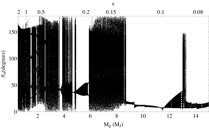
Figure 1: “Bifurcation” diagram of the spin-orbit misalignment angle versus planet mass and the adiabaticity parameter $\epsilon$. For each planet mass $M_{p}$, we evolve the secular orbital evolution equations including the effects of short-range forces (periastron advances due to General Relativity, the stellar quadrupole, and the planet’s rotational bulge and tidal distortion) together with the stellar spin precession equation, starting with $\theta_{\rm{sl}}=0$, for $\sim\!1500$ Lidov-Kozai cycles, and record $\theta_{\rm{sl}}$ every time the orbital eccentricity reaches a maximum. The parameters for this plot are $a=1$ AU, $a_{b}=200$ AU, $e_{0}=0.01$, $\theta^{0}_{\rm lb}=85^{\circ}$, $\hat{\Omega}_{\star}=0.03$. This figure is an extended version of Fig. 4 of Storch, Anderson & Lai (2014), demonstrating the complexity of the trans-adiabatic and even the adiabatic regimes of the spin dynamics.

Widespread chaos in dynamical systems can be understood as arising from overlaps of resonances in the phase space (Chirikov 1979). What are the resonances underlying the chaotic spin behaviour found in SAL and Fig. 1? Since $\Omega_{\rm{pl}}$ and $\Omega_{\rm{ps}}$ are both strong functions of time, the answer to this question is not obvious a priori, even in the ideal case when the planetary orbit undergoes strictly periodic Lidov-Kozai oscillations. Using Hamiltonian perturbation theory, we show in this paper that a spin-orbit resonance occurs when the time-averaged spin precession frequency equals an integer multiple of the Lidov-Kozai oscillation frequency. We then demonstrate that overlapping resonances can indeed explain the onset of chaos in the dynamics of stellar spin, more specifically the “adiabatic” to “trans-adiabatic” transition. We also show that many of the intricate “quasi-chaotic” features found numerically in the “adiabatic” regime can be understood from overlapping resonances. Finally we show that the consideration of resonances can lead to a novel “adiabatic resonance advection” phenomenon when tidal decay of the planetary orbit is included.

The chaotic dynamics of stellar spin studied in this paper has some resemblance to the well-known problem of obliquity dynamics of Mars and other terrestrial planets (Laskar & Robutel 1993; Touma & Wisdom 1993; see Li & Batygin 2014). In that problem, a spin-orbit resonance arises when the spin precession frequency $\Omega_{\rm{ps}}$ of Mars around its orbital axis $\hat{{\bf L}}$ driven by the Sun matches one of the eigen-frequencies ($\Omega_{\rm{pl}}$’s) for the variation of $\hat{{\bf L}}$ due to interactions with other planets. Only a small number of $\Omega_{\rm{pl}}$’s are relevant in the Solar System, and except for the $\cos\theta_{\rm{sl}}$ factor, $\Omega_{\rm{ps}}$ is approximately constant in time. Thus the analysis of overlapping resonances is relatively straightforward. For the problem studied in this paper, by contrast, both $(\Omega_{\rm{ps}}/\cos\theta_{\rm{sl}})$ and $\Omega_{\rm{pl}}$ are strong functions of time, so the dynamics of the stellar spin axis exhibits a much richer set of behaviors.

Our paper is organized as follows. In Section 2, we review the physical system and its ingredients. In Section 3, we develop a Hamiltonian formulation of the problem, and derive the resonance condition for spin-orbit coupling. In Section 4, we discuss the behaviour of the system under the influence of a single resonance. In Section 5, we demonstrate the onset of chaos in the presence of two or more overlapping resonances, and derive the overlap criterion. In Section 6, we consider the full Lidov-Kozai driven spin precession problem, and demonstrate that resonance overlaps can explain the onset of chaos, as well as other “quasi-chaotic” features in the spin evolution. In Section 7, we consider the effect of a slowly evolving adiabaticity parameter, as a simplified model of tidal dissipation, and present a proof of concept for understanding the novel “adiabatic resonance advection” phenomenon. We summarize our key findings in Section 8.

2 Review of the Physical System and Ingredients

2.1 Lidov-Kozai (LK) Oscillations

We consider a planet of mass $M_{p}$ in orbit around a host star of mass $M_{\star}$ (with $M_{\star}\gg M_{p}$), and a distant companion of mass $M_{b}$. The host star and companion are in a static orbit with semi-major axis $a_{b}$, eccentricity $e_{b}$, and angular momentum axis $\hat{{\bf L}}_{b}$, which defines the invariant plane of the system. The planet’s orbit has semi-major axis $a$, eccentricity $e$, angular momentum axis $\hat{{\bf L}}$ and inclination $\theta_{\rm{lb}}$ (the angle between $\hat{{\bf L}}$ and $\hat{{\bf L}}_{b}$). In the Lidov-Kozai (LK) mechanism, the quadrupole potential of the companion causes the orbit of the planet to undergo oscillations of both $e$ and $\theta_{\rm{lb}}$, as well as nodal precession ($\dot{\Omega}$) and pericenter advance ($\dot{\omega}$), while conserving ${\bf L}\cdot\hat{{\bf L}}_{b}$. The equations governing these oscillations are given by

$${de\over dt} = t_{k}^{-1}{15\over 8}e\sqrt{1-e^{2}}\sin 2\omega\sin^{2}\theta_{\rm{lb}},$$ (3)

$${d\Omega\over dt} = t_{k}^{-1}{3\over 4}{\cos\theta_{\rm{lb}}\left(5e^{2}\cos^{2}\omega-4e^{2}-1\right)\over\sqrt{1-e^{2}}},$$ (4)

$${d\theta_{\rm{lb}}\over dt} = -t_{k}^{-1}{15\over 16}{e^{2}\sin 2\omega\sin 2\theta_{\rm{lb}}\over\sqrt{1-e^{2}}},$$ (5)

$${d\omega\over dt} = t_{k}^{-1}{3\left[2(1-e^{2})+5\sin^{2}\omega(e^{2}-\sin^{2}\theta_{\rm{lb}})\right]\over 4\sqrt{1-e^{2}}},$$ (6)

where $t_{k}^{-1}$ is the characteristic frequency of oscillation, given by

$$t_{k}^{-1}={n\over(1-e_{b}^{2})^{3/2}}\left(\frac{M_{b}}{M_{\star}}\right)\left(\frac{a}{a_{b}}\right)^{3},$$ (7)

where $n=\sqrt{GM_{\star}/a^{3}}$ is the planet’s mean motion. In this paper, we neglect all effects associated with short-range forces (General Relativity, tidal interaction, etc) and the octupole potential from the binary.

Equations (3)-(6) admit two types of analytical solutions, distinguished by whether the argument of pericenter $\omega$ circulates or librates. In the present work we will consider only the circulating case by taking $\omega=0$ at $t=0$. The conservation of the projected angular momentum ${\bf L}\cdot\hat{{\bf L}}_{b}$ gives

$$x\cos^{2}\theta_{\rm{lb}}=x_{0}\cos^{2}\theta_{\rm{lb}}^{0}\equiv h,$$ (8)

where

$$x\equiv 1-e^{2},$$ (9)

and energy conservation gives

$$e^{2}(5\sin^{2}\theta_{\rm{lb}}\sin^{2}\omega-2)=-2e_{0}^{2}.$$ (10)

For the initial eccentricity $e_{0}\approx 0$, the above equations imply that the maximum eccentricity occurs at $\omega=\pi/2,\,3\pi/2$, where $\sin^{2}\theta_{\rm{lb}}=2/5$ and

$$e_{\rm max}\simeq\left(1-{5\over 3}\cos^{2}\theta_{\rm{lb}}^{0}\right)^{1/2}.$$ (11)

Combining eqs. (8)-(10) with eq. (3), the time evolution of eccentricity can be solved explicitly (Kinoshita & Nakai 1999):

$$x=x_{0}+(x_{1}-x_{0}){\rm cn}^{2}(\theta,k^{2}),$$ (12)

where

$$\theta = \frac{K}{\pi}\left(n_{e}t+\pi\right),$$ (13)

$$n_{e} = t_{k}^{-1}\frac{6\pi\sqrt{6}}{8K}\sqrt{x_{2}-x_{1}},$$ (14)

$$k^{2} = \frac{x_{0}-x_{1}}{x_{2}-x_{1}}.$$ (15)

In the above expressions ${\rm cn}(\theta,k^{2})$ is the Jacobi elliptic ${\rm cn}$ function with modulus $k^{2}$, $n_{e}$ is the “mean motion” for the eccentricity variation (i.e. $2\pi/n_{e}$ is the period of the eccentricity oscillations), $K$ is the complete elliptic integral of the first kind with modulus $k^{2}$, $x_{0}$ is the value of $x$ at $t=0$, and $x_{1}$ and $x_{2}$ ($x_{1}<x_{2}$) are solutions to the quadratic equation

$$x_{1,2}^{2}-\frac{1}{3}\left(5+5h-2x_{0}\right)x_{1,2}+\frac{5}{3}h=0,$$ (16)

obtained from eqs. (8)-(10) with $\sin^{2}\omega=1$. The other orbital elements can be expressed as a function of $x$. Note that the period of $\omega$ circulation ($\omega$ goes from 0 to $2\pi$) is $4\pi/n_{e}$.

For the remainder of this work, we use a single $x(t)$ solution in our analysis, corresponding to $e_{0}=0.01$ (so $x_{0}=1-(0.01)^{2}$) and $\theta^{0}_{\mathrm{lb}}=85^{\circ}$.

2.2 Stellar spin precession

Because of the rotation-induced oblateness, the star is torqued by the planet, causing its spin axis $\hat{{\bf S}}$ to precess around the planet’s orbital axis $\hat{{\bf L}}$ according to the equation

$$\frac{d\hat{{\bf S}}}{dt}=\Omega_{\rm{ps}}\hat{{\bf L}}\times\hat{{\bf S}},$$ (17)

where the precession frequency $\Omega_{\rm{ps}}$ is given by

$$\Omega_{\rm{ps}}=-\frac{3GM_{p}(I_{3}-I_{1})}{2a^{3}(1-e^{2})^{3/2}}\frac{\cos\theta_{\rm{sl}}}{S}.$$ (18)

Here $I_{3}$ and $I_{1}$ are the principal moments of inertia of the star, $S$ is the magnitude of the spin angular momentum, and $\theta_{\rm{sl}}$ is the angle between $\hat{{\bf S}}$ and $\hat{{\bf L}}$. Our goal is to characterize how $\theta_{\rm{sl}}$ changes as a function of time as the planet’s orbit undergoes LK oscillations. Since $e$ changes during the LK cycle, we write the spin precession frequency as

$$\Omega_{\rm{ps}}(t)\equiv-\alpha(t)\cos\theta_{\rm{sl}}=-\frac{\alpha_{0}}{x^{3/2}}\cos\theta_{\rm{sl}},$$ (19)

where

$$\alpha_{0} = {3GM_{p}(I_{3}-I_{1})\over 2a^{3}I_{3}\Omega_{\star}}$$ (20)

$$= 1.19\times 10^{-8}\left({2\pi\over 1\mathrm{yr}}\right)\left({2k_{q}\over k_{\star}}\right)\left({10^{3}M_{p}\over M_{\star}}\right)\left({\hat{\Omega}_{\star}\over 0.05}\right)\times$$

$$\times\left({a\over 1\mathrm{AU}}\right)^{-3}\left({M_{\star}\over M_{\odot}}\right)^{1/2}\left({R_{\star}\over R_{\odot}}\right)^{3/2}.$$

Here we have used $(I_{3}-I_{1})\equiv k_{q}M_{\star}R_{\star}^{2}\hat{\Omega}_{\star}^{2}$, with $\hat{\Omega}_{\star}=\Omega_{\star}/(GM_{\star}/R_{\star}^{3})^{1/2}$ the dimensionless stellar rotation rate, and $S=I_{3}\Omega_{s}\equiv k_{\star}M_{\star}R_{\star}^{2}\Omega_{\star}$. For a solar-type star, $k_{q}\approx 0.05$, and $k_{\star}\approx 0.1$ (Claret 1992).

During the LK cycle, the planet’s orbital axis $\hat{{\bf L}}$ changes in two distinct ways: nodal precession around $\hat{{\bf L}}_{b}$ at the rate $\Omega_{\rm{pl}}(t)=\dot{\Omega}$, and nutation at the rate $\dot{\theta}_{\rm lb}(t)$. Each of these acts as a driving force for the stellar spin. The variation of $\theta_{\rm{lb}}(t)$ plays an important role as well since it affects $\hat{{\bf L}}(t)$ directly [see Eq. (30) below]. Note that the back-reaction torque from the stellar quadrupole on the orbit also acts to make $\hat{{\bf L}}$ precess around $\hat{{\bf S}}$; we neglect this back-reaction throughout this paper in order to focus on the spin dynamics with “pure” orbital LK cycles. Based on the analytical LK solution given in the previous sub-section, we find $\Omega_{\rm{pl}}$ is given by

$$\Omega_{\rm{pl}}=\dot{\Omega}=\Omega_{\rm pl,0}\left[1-\frac{2(x_{0}-h)}{x-h}\right],$$ (21)

with $x$ is given by Eq. (12) and

$$\Omega_{\rm pl,0}=\frac{3}{4t_{k}}\sqrt{h}\simeq\frac{3}{4t_{k}}\left|\cos\theta^{0}_{\rm lb}\right|,$$ (22)

where the second equality assumes $e_{0}\simeq 0$. The angle $\theta_{\rm{lb}}$ and its derivative are given by $\cos\theta_{\rm{lb}}=\sqrt{h/x}$ and $\dot{\theta}_{\rm lb}=\dot{x}\cos\theta_{\rm{lb}}/(2x\sin\theta_{\rm{lb}})$. Note that $\Omega_{\rm{pl}}(t)<0$. The quantity $\Omega_{\rm pl,0}$ specifies the value of $\left|\Omega_{\rm{pl}}\right|$ at $e=e_{0}\simeq 0$, and is explicitly given by

$$\Omega_{\rm pl,0} \simeq \frac{3}{4}\left({2\pi\over 10^{6}\mathrm{yr}}\right)\left({M_{b}\over M_{\star}}\right)\left({M_{\star}\over M_{\odot}}\right)^{1/2}\left({a\over 1\mathrm{AU}}\right)^{3/2}\times$$ (23)

$$\times\left({a_{b}\over 100\mathrm{AU}}\right)^{-3}{\left|\cos\theta^{0}_{\rm lb}\right|\over(1-e_{b}^{2})^{3/2}},$$

for $x_{0}=1-e_{0}^{2}\simeq 1$. Taking the ratio of this and Eq. (20) yields the adiabaticity parameter

$$\epsilon={\Omega_{\rm pl,0}\over\alpha_{0}},$$ (24)

as given in Section 1 [see Eq. (2)].

3 Hamiltonian Formulation of Spin Dynamics and Resonances

3.1 The Spin Hamiltonian

In the inertial frame, the Hamiltonian governing the dynamics of stellar spin ${\bf S}=S\hat{{\bf S}}$ is

$$H={S^{2}\over 2I_{3}}+{GM_{p}(I_{3}-I_{1})\over 4a^{3}(1-e^{2})^{3/2}}\left[1-3(\hat{{\bf S}}\cdot\hat{{\bf L}})^{2}\right].$$ (25)

The first term is the (constant) rotational kinetic energy and will be dropped henceforth, and the second term is the orbital-averaged interaction energy between the planet and stellar quadrupole. Since the evolution of the orbital eccentricity $e(t)$ is fixed, we only need to consider the last term in Eq. (25):

$$H_{0}\equiv-{1\over 2}\alpha(t)S\left(\hat{{\bf S}}\cdot\hat{{\bf L}}\right)^{2}.$$ (26)

Noting that $\hat{{\bf S}}\cdot\hat{{\bf L}}_{b}$ and $\phi_{s}$ (the precessional phase of $\hat{{\bf S}}$ around $\hat{{\bf L}}_{b}$) are conjugate variables, we can check that the Hamiltonian equations for $H_{0}$ lead to Eq. (17).

Since we are interested in the variation of $\theta_{\rm{sl}}$, it is convenient to work in the rotating frame in which $\hat{{\bf L}}$ is a constant. In this frame, the Hamiltonian takes the form (cf. Kinoshita 1993)

$$H_{\rm rot}=H-{\bf R}\cdot{\bf S},$$ (27)

where the rotation “matrix” is

$${\bf R}=\Omega_{\rm{pl}}\hat{{\bf L}}_{b}+{\dot{\theta}}_{\rm lb}\left({\hat{{\bf L}}_{b}\times\hat{{\bf L}}\over\sin\theta_{\rm{lb}}}\right).$$ (28)

To write down the explicit expression for $H_{\rm rot}$, we set up a Cartesian coordinate system with the $z$-axis along $\hat{{\bf L}}$, and the $x$-axis pointing to the ascending node of the planet’s orbit in the invariant plane (the plane perpendicular to $\hat{{\bf L}}_{b}$). The spin axis is characterized by $\theta_{\rm{sl}}$ and the precessional phase $\phi$ (the longitude of the node of the star’s rotational equator in the $xy$-plane), such that

$$\hat{{\bf S}}=\sin\theta_{\rm{sl}}\left(\sin\phi\,{\hat{x}}-\cos\phi\,{\hat{y}}\right)+\cos\theta_{\rm{sl}}\,{\hat{z}}.$$ (29)

Setting $S=1$ and suppressing the subscript “rot”, we have

$$H=-{1\over 2}\alpha(t)\left(\cos\theta_{\rm{sl}}\right)^{2}-\dot{\theta}_{\rm lb}(t)\sin\theta_{\rm{sl}}\sin\phi$$

$$\quad-\Omega_{\rm{pl}}(t)\Bigl{[}\cos\theta_{\rm{lb}}(t)\cos\theta_{\rm{sl}}-\sin\theta_{\rm{lb}}(t)\sin\theta_{\rm{sl}}\cos\phi\Bigr{]},$$ (30)

Note that $\phi$ and $\cos\theta_{\rm{sl}}$ are the conjugate pair of variables we wish to solve for. Since in this work we focus on the behavior of the system close to the adiabatic regime, in general the first term in the Hamiltonian dominates, while the others can be treated as perturbations. In the limit of no perturbation, the zeroth order Hamiltonian $H_{0}\equiv-{1\over 2}\alpha(t)\cos^{2}\theta_{\rm{sl}}$ indeed conserves $\cos\theta_{\rm{sl}}$, as it should based on the arguments given in Section 1.

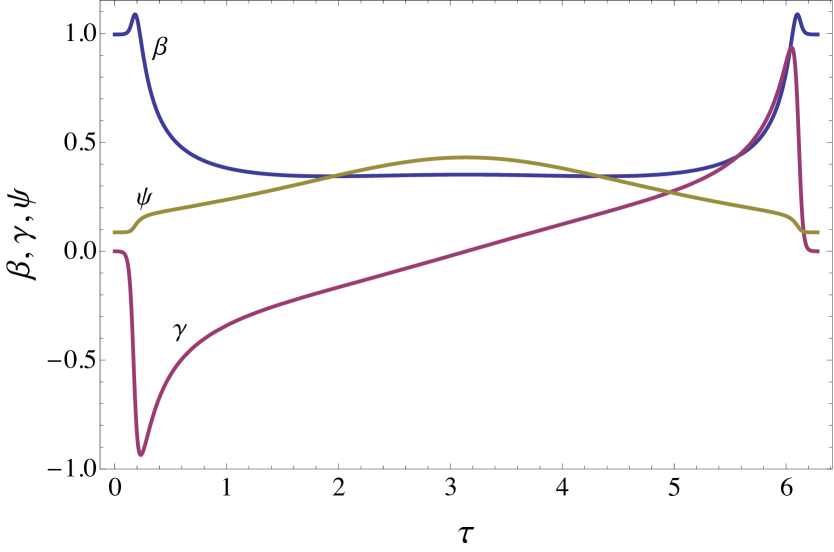
Figure 2: Plots of the “shape” functions $\beta(\tau)$ (blue), $\gamma(\tau)$ (red), and $\psi(\tau)$ (brown), for $x_{0}=1-0.01^{2}$ and $\cos\theta^{0}_{\rm lb}=85^{\circ}$.

3.2 The Renormalized Hamiltonian

The equations of motion for $\phi$ and $\cos\theta_{\rm{sl}}$ can be derived from the Hamiltonian (30), and are given by

$$\frac{d\phi}{dt}=-\alpha(t)\cos\theta_{\rm{sl}}+\dot{\theta}_{\rm lb}(t)\frac{\cos\theta_{\rm{sl}}}{\sin\theta_{\rm{sl}}}\sin\phi$$

$$\qquad\quad-\Omega_{\rm{pl}}(t)\left[\cos\theta_{\rm{lb}}(t)+\sin\theta_{\rm{lb}}(t)\frac{\cos\theta_{\rm{sl}}}{\sin\theta_{\rm{sl}}}\cos\phi\right],$$ (31)

$$\frac{d\cos\theta_{\rm{sl}}}{dt}=\Omega_{\rm{pl}}(t)\sin\theta_{\rm{lb}}(t)\sin\theta_{\rm{sl}}\sin\phi$$

$$\qquad\quad+\dot{\theta}_{\rm lb}(t)\sin\theta_{\rm{sl}}\cos\phi.$$ (32)

These equations can be simplified by introducing a rescaled time variable $\tau$ such that $d\tau\propto\alpha(t)dt$, i.e.,

$$\tau(t)=\frac{n_{e}}{\bar{\alpha}}\int_{0}^{t}\alpha(t^{\prime})dt^{\prime},$$ (33)

where

$$\bar{\alpha}\equiv\frac{n_{e}}{2\pi}\int_{0}^{2\pi/n_{e}}\!\alpha(t)dt.$$ (34)

Here the factor of $n_{e}/\bar{\alpha}$ is used to ensure that all of the time-dependent forcing functions introduced in Section 2 have a period of $2\pi$ in $\tau$-space, for convenience. The equations of motion in $\tau$ space are then given by

$$\frac{d\phi}{d\tau}=\frac{\bar{\alpha}}{n_{e}}\biggl{\{}-\cos\theta_{\rm{sl}}+\frac{\dot{\theta}_{\rm lb}(\tau)}{\alpha(\tau)}\frac{\cos\theta_{\rm{sl}}}{\sin\theta_{\rm{sl}}}\sin\phi$$

$$\quad~{}~{}-\frac{\Omega_{\rm{pl}}(\tau)}{\alpha(\tau)}\Bigl{[}\cos\theta_{\rm{lb}}(\tau)+\sin\theta_{\rm{lb}}(\tau)\frac{\cos\theta_{\rm{sl}}}{\sin\theta_{\rm{sl}}}\cos\phi\Bigr{]}\!\biggr{\}},$$ (35)

$$\frac{d\cos\theta_{\rm{sl}}}{d\tau}=\frac{\bar{\alpha}}{n_{e}}\biggl{\{}\frac{\Omega_{\rm{pl}}(\tau)}{\alpha(\tau)}\sin\theta_{\rm{lb}}(\tau)\sin\theta_{\rm{sl}}\sin\phi$$

$$\quad~{}~{}+\frac{\dot{\theta}_{\rm lb}(\tau)}{\alpha(\tau)}\sin\theta_{\rm{sl}}\cos\phi\biggr{\}}.$$ (36)

The corresponding Hamiltonian is

$$H^{\prime}(p,\phi,\tau)=\frac{\bar{\alpha}}{n_{e}}\biggl{\{}-\frac{1}{2}p^{2}+\epsilon\psi(\tau)\,p$$

$$\qquad~{}~{}-\epsilon\sqrt{1-p^{2}}\,\Bigl{[}\beta(\tau)\cos\phi+\gamma(\tau)\sin\phi\Bigr{]}\biggr{\}},$$ (37)

where we have defined $p\equiv\cos\theta_{\rm{sl}}$, and

$$\epsilon\beta(\tau)=-\frac{\Omega_{\rm{pl}}(\tau)}{\alpha(\tau)}\sin\theta_{\rm{lb}}(\tau),$$ (38)

$$\epsilon\gamma(\tau)=\frac{\dot{\theta}_{\rm lb}(\tau)}{\alpha(\tau)},$$ (39)

$$\epsilon\psi(\tau)=-\frac{\Omega_{\rm{pl}}(\tau)}{\alpha(\tau)}\cos\theta_{\rm{lb}}(\tau).$$ (40)

Since $\epsilon={\Omega_{\rm pl,0}/\alpha_{0}}$ [see Eq. (24)], the functions $\beta(\tau)$, $\gamma(\tau)$ and $\psi(\tau)$ depend only on the “shape” of the orbit, i.e., on $e(\tau)$ (with $\tau$ varying from 0 to $2\pi$). For a given $\theta_{\rm{lb}}^{0}$ (and $e_{0}\simeq 0$), these functions are fixed and do not depend on any other parameters. Figure 2 depicts these functions for $\theta_{\rm{lb}}^{0}=85^{\circ}$.

3.3 Fourier Decomposition and Resonances

Figure 3: Sum of the Fourier coefficients as a function of the resonance number $N$. Filled circles are for positive $\beta_{N}+\gamma_{N}$, and open circles are for negative $\beta_{N}+\gamma_{N}$. Note that $\beta_{-N}=\beta_{N}$, while $\gamma_{-N}=-\gamma_{N}$, which accounts for the lack of symmetry across $N=0$.

We now expand $\beta(\tau),\gamma(\tau)$, and $\psi(\tau)$ in Fourier series. Since $\beta$ and $\psi$ are symmetric with respect to $\tau=\pi$, while $\gamma$ is anti-symmetric (see Fig. 2), we have

$$\beta(\tau)=\sum_{M=0}^{\infty}\beta_{M}\cos M\tau,$$ (41)

$$\gamma(\tau)=\sum_{M=1}^{\infty}\gamma_{M}\sin M\tau,$$ (42)

$$\psi(\tau)=\sum_{M=0}^{\infty}\psi_{M}\cos M\tau.$$ (43)

Obviously, $\beta_{M}$, $\gamma_{M}$ and $\psi_{M}$ depend only on the “shape” of the orbit $e(\tau)$. The Hamiltonian (37) becomes

$$H^{\prime}=\frac{\bar{\alpha}}{n_{e}}\biggl{\{}-\frac{1}{2}p^{2}+\epsilon\,\psi_{0}\,p+\epsilon\,p\sum_{M=1}^{\infty}\psi_{M}\cos Mt$$

$$\qquad~{}-\frac{\epsilon}{2}\sqrt{1-p^{2}}\sum_{M=0}^{\infty}\Bigl{[}(\beta_{M}+\gamma_{M})\cos(\phi-M\tau)$$

$$\qquad\quad\quad\quad\quad+(\beta_{M}-\gamma_{M})\cos(\phi+M\tau)\Bigr{]}\biggr{\}}.$$ (44)

Note that $\gamma_{0}$ is not defined in Eq. (42). For convenience of notation, we will set $\gamma_{0}=\beta_{0}$ [see discussion following Eq. (53)].

A resonance occurs when the argument of the cosine function, $(\phi\pm M\tau)$, in the Hamiltonian (44) is slowly varying, i.e., when ${d\phi}/{d\tau}=N$, where $N$ is a positive or negative integer. In the perturbative regime ($\epsilon\ll 1$) of interest in this paper, the Hamiltonian is dominated by $H_{0}=(\bar{\alpha}/n_{e})(-p^{2}/2)$, and we have ${d\phi}/{d\tau}\simeq-\bar{\alpha}p/n_{e}$. So the resonance condition becomes

$${\bar{\Omega}}_{\rm ps}=-\bar{\alpha}\cos\theta_{\rm{sl}}=Nn_{e},\qquad{\rm with}~{}~{}N=0,\pm 1,\pm 2,\pm 3,\cdots$$ (45)

i.e. the averaged stellar precession frequency ${\bar{\Omega}}_{\rm ps}$ equals an integer multiple of the mean eccentricity oscillation frequency in the LK cycle. Note that, since $\cos\theta_{\rm{sl}}$ spans the range $\{-1,1\}$, this means that for any given value of $\bar{\alpha}$ and of $n_{e}$ there exist multiple resonances. We may then define the zeroth-order resonant momentum corresponding to each resonance as

$$p_{N}=\left(\cos\theta_{\rm sl}\right)_{N}=-\frac{Nn_{e}}{\bar{\alpha}}.$$ (46)

Since $|p_{N}|$ cannot exceed $1$, we also see that there exists a “maximum resonance order”,

$$N_{\rm max}=\left\lfloor\frac{\bar{\alpha}}{n_{e}}\right\rfloor=\left\lfloor\frac{1}{\epsilon}\mathcal{N}\left(\cos\theta^{0}_{\rm lb};e_{0}\right)\right\rfloor,$$ (47)

such that $N=N_{\rm max}$ is the maximum allowed positive resonance, and $N=-N_{\rm max}$ is the maximum allowed negative resonance. Note that the resonant momentum $p_{N}$ can be written as

$$p_{N}\simeq-{N\over N_{\rm max}}.$$ (48)

Thus, the stellar spin evolution is perturbed by a set of $(2N_{\rm max}+1)$ resonances. The function $\mathcal{N}$ depends mainly on $\cos\theta^{0}_{\rm lb}$, and weakly on $e_{0}$ (assuming $e_{0}\ll 1$). For $\theta^{0}_{\rm lb}=85^{\circ}$ (adopted for our numerical examples in this paper), we find $\mathcal{N}=0.98$.

The $N=-N_{\rm max}$ resonance is of particular interest, as it is the closest resonance to $p_{N}=1$, the aligned configuration. Thus, if a star-planet system is born with the stellar spin axis and the planet orbital axis aligned, this resonance is the one that most directly influences the stellar spin evolution This will be discussed in detail in Section 6.

We may now ask what happens if the resonance condition is satisfied: how are the dynamics of stellar spin precession affected by one - or more - resonances? To make the solution tractable analytically, we must make some simplifying assumptions. We assume $\epsilon$ is small, i.e. the system is in or close to the adiabatic regime. As a corollary, we assume that individual resonances do not affect each other significantly, i.e., that we may analyze the resonances one at a time rather than consider the coupling between them.

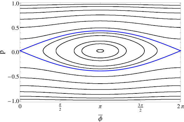
Figure 4: Sample constant-energy curves for the $N=0$ single-resonance Hamiltonian [given by Eq. (53)], constructed by starting with a variety of initial conditions (corresponding to unique values of E) and evolving the equations of motion derived from the Hamiltonian. The blue line shows the analytical prediction for the separatrix. The adiabaticity parameter is $\epsilon=0.1$, i.e. $\alpha_{0}=10\Omega_{\rm pl,0}$.

4 Dynamics of a Single Resonance

To examine the dynamics of a particular single resonance (labeled by $N$, which can be either positive or negative), it is useful to transform the Hamiltonian into the frame of reference in which that resonance is stationary. To this end, we perform a canonical transformation to the new coordinates $(\bar{\phi},\bar{p})$ such that $\bar{\phi}=\phi-N\tau$. Using the generating function $F_{2}=(\phi-N\tau)\bar{p}$, we then find

$$\bar{p}=p,\quad\bar{\phi}=\phi-N\tau,$$ (49)

$$\bar{H^{\prime}}=H^{\prime}\left[\phi(\bar{\phi}),p(\bar{p});\tau\right]-N\bar{p}.$$ (50)

Thus the transformed Hamiltonian is

$$\bar{H^{\prime}}=\frac{\bar{\alpha}}{n_{e}}\biggl{\{}-\frac{1}{2}p^{2}-\frac{n_{e}}{\bar{\alpha}}Np+\epsilon\,p\sum_{M=0}^{\infty}\psi_{M}\cos M\tau$$

$$\qquad-\frac{\epsilon}{2}\sqrt{1-p^{2}}\sum_{M=0}^{\infty}\Bigl{[}(\beta_{M}+\gamma_{M})\cos\left[\bar{\phi}-(M-N)\tau\right]$$

$$\quad\quad\quad\quad\quad+(\beta_{M}-\gamma_{M})\cos\left[\bar{\phi}+(M+N)\tau\right]\Bigr{]}\biggr{\}},$$ (51)

where we have dropped the bar over $p$, since $\bar{p}=p$. We now take the average

$$\tilde{H}_{N}=\frac{1}{2\pi}\int_{0}^{2\pi}\bar{H^{\prime}}d\tau.$$ (52)

Note that all the terms in the sums are rapidly varying and are averaged out except the $M=0$ term in the first sum, the $M=N$ term (when $N>0$) in the second sum, and/or the $M=-N$ term (when $N<0$) in the third sum. We then have

$$\bar{H}_{N}=\frac{\bar{\alpha}}{n_{e}}\biggl{[}-\frac{1}{2}p^{2}-\frac{n_{e}}{\bar{\alpha}}Np$$

$$\qquad+\epsilon\,\psi_{0}\,p-\frac{\epsilon}{2}\sqrt{1-p^{2}}\,(\beta_{N}+\gamma_{N})\cos\bar{\phi}\biggr{]},$$ (53)

where we have used $\beta_{-N}=\beta_{N}$ and $\gamma_{-N}=-\gamma_{N}$. In order to ensure that this expression is valid for all $N$’s (including $N=0$), we set $\gamma_{0}=\beta_{0}$.

The Hamiltonian (53) shows that the sum of Fourier coefficients $(\beta_{N}+\gamma_{N})$ plays a key role in determining the property of the $N$-resonance. Figure 3 plots $\left(\beta_{N}+\gamma_{N}\right)$ versus $N$, showing that it oscillates from positive to negative in a ringdown fashion. This oscillatory behaviour arises from individual ringdowns in $\beta_{N}$ and $\gamma_{N}$, as well as from interference between the $\beta_{N}$ and $\gamma_{N}$ terms.

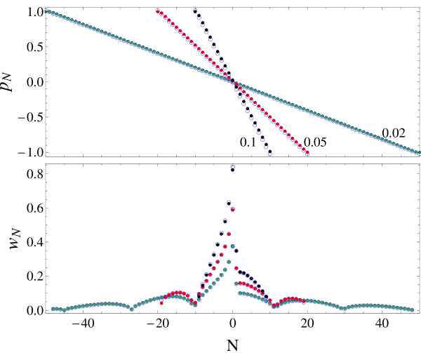
Figure 5: Comparison of the exact resonance locations (upper panel) and widths (bottom panel) obtained by solving Eq. (53) (filled circles) with simple analytical estimates (open circles). Three different values of $\epsilon$ are considered: $\epsilon=0.1$ (blue points), $\epsilon=0.05$ (red points), and $\epsilon=0.02$ (green points). The agreement between the exact calculation and simple estimates is quite good, and gets better with smaller $\epsilon$.

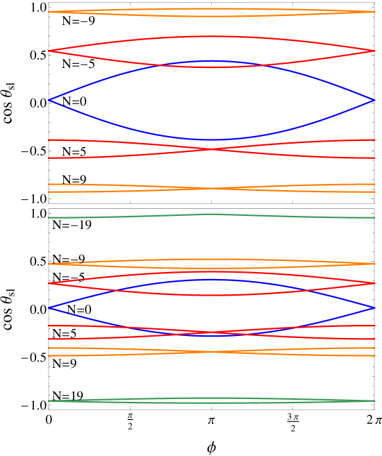
Figure 6: Sample separatrices for resonances of different $N$’s, for $\epsilon=0.1$ (top) and $\epsilon=0.05$ (bottom). The top panel has $N_{\rm max}=9$, and the bottom panel has $N_{\rm max}=19$.

Since the Hamiltonian (53) is not explicitly dependent on time, energy conservation holds, i.e.

$$\bar{H}_{N}(\bar{\phi},p)=\bar{H}_{N}(\bar{\phi}_{0},p_{0})\equiv E,$$ (54)

for a trajectory that starts at $(\bar{\phi}_{0},p_{0})$. This equation is quartic which can be solved for $p(\bar{\phi};E)$. Figure 4 shows the constant-energy curves in the phase space for $N=0$, illustrating the major features of the solution. The trajectories come in two distinct flavors: those that circulate, i.e. cover the entire range of $\bar{\phi}$ and do not cross $p=p_{N}$ [see Eq. (46)], and those that librate, i.e. are confined to some limited range of $\bar{\phi}$. The center of the librating island is the true location of the resonance, which is a stable fixed point of the equations of motion. Separating the librating and circulating regions of the phase space is a special curve known as the separatrix, which connects two saddle fixed points. The width of the separatrix (in the $p$ axis) defines the width of the resonance.

To derive a simple expression for the resonance width, we may simplify the Hamiltonian (53) further by expanding it around $p=p_{N}$, where $p_{N}$ is the zeroth-order resonant momentum given by Eq. (46). We take $p=p_{N}+\delta p$, assume the terms proportional to $\epsilon$ are already small, and expand Eq. (53) to second order in $\delta p$:

$$\bar{H}_{N}\simeq\frac{\bar{\alpha}}{n_{e}}\biggl{[}-\frac{1}{2}\delta p^{2}-\frac{\epsilon}{2}\sqrt{1-p_{N}^{2}}\,(\beta_{N}+\gamma_{N})\cos\bar{\phi}\biggr{]},$$ (55)

where constant terms (which do not depend on $\delta p$) have been dropped. Equation (55) is the Hamiltonian of a simple Harmonic oscillator. The resonance width is given by

$$w_{N}\simeq 2\left[2\,\epsilon\,|\beta_{N}+\gamma_{N}|\sqrt{1-p_{N}^{2}}\right]^{1/2}.$$ (56)

Figure 5 shows a comparison of the exact locations of the resonances (the fixed points of Eq. 53) with the unperturbed value $p_{N}$ [see Eq. (46)], as well as a comparison of the exact widths of the resonances with Eq. (56). We see that the approximate Hamiltonian (55) reproduces the resonance properties of the full Hamiltonian (53) accurately. Note that the resonance width depends on the sum of fourier coefficients $|\beta_{N}+\gamma_{N}|$, and since $\beta$ is symmetric while $\gamma$ is antisymmetric with respect to $N$, the positive and negative resonances do not have the same widths. Furthermore, since $\left(\beta_{N}+\gamma_{N}\right)$ goes through zero several times in the interval $N\in\{-100,100\}$, the resonance width is non-monotonic as a function of $N$.

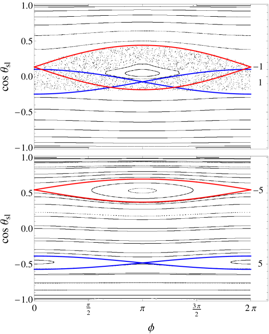
Figure 7: Surfaces of section for two different pairs of resonances. Top panel : $N=1,\,M=-1$. Bottom panel : $N=5,\,M=-5$. The adiabaticity parameter is $\epsilon=0.1$. The red and blue curves in each panel show the analytically computed separatrices for each of the resonances, using the method of Section 4 (i.e. each resonance is analyzed separately).

Figure 6 shows several separatrices for resonances of different orders (i.e. different $N$s) obtained by solving the full Hamiltonian (53), for two different values of $\epsilon$. (Note we vary $\epsilon$ by varying $\alpha_{0}$ while keeping $\Omega_{\rm pl,0}$ fixed; this means that the “shape” functions are unchanged.) Figure 6 illustrates several different features of the separatrices. First, decreasing $\epsilon$ tends to decrease the displacement of individual resonances from $p=0$. Each resonance is centered at $p\simeq p_{N}\simeq-N/N_{\rm max}$. Since the maximum order of resonance, $N_{\rm max}$ (recall that no resonance is possible for $|N|>N_{\rm max}$; see Section 3.3), is inversely proportional to $\epsilon$ (Eq. 47), we have $|p_{N}|\propto\epsilon$. Second, the general trend is that at smaller $\epsilon$ all the resonances are narrower, though this is not precisely true because $p_{N}$ also depends on $\epsilon$ [see Eq. (56)]. Finally, the position of the resonance in the $\phi$ coordinate depends on the sign of $(\beta_{N}+\gamma_{N})$: if $(\beta_{N}+\gamma_{N})<0$, the resonance is located at $\phi=\pi$, and if $(\beta_{N}+\gamma_{N})>0$ – at $\phi=0$. Since $\gamma_{-N}=-\gamma_{N}$, this usually implies that there are significant differences between resonances with $N>0$ and those with $N<0$.

To summarize, given a particular value of the adiabaticity parameter $\epsilon$, the stellar spin is perturbed by a set of resonances $d\phi/d\tau=N$ with $N\in\{-N_{\rm max},N_{\rm max}\}$, where $N_{\rm max}$ is given by Eq. (47). Each resonance governs the stellar spin evolution in the vicinity of $\cos\theta_{\rm{sl}}=p_{N}$, with $p_{N}$ approximately given by Eq. (46), and the width of the governed region approximately given by Eq. (56). As $\epsilon$ decreases (the system becomes more adiabatic), $N_{\rm max}$ increases, $|p_{N}|\simeq|N|/N_{\rm max}$ (for a given $N$) decreases (the resonance locations move closer to $p=0$), and the width of the resonance generally decreases. For a given $\epsilon$, the width of the resonance is a non-monotonic function of $N$ because of its dependence on $(\beta_{N}+\gamma_{N})$.

5 Onset of Chaos: Two or More Resonances

We now consider a Hamiltonian of the form

$$H=\frac{\bar{\alpha}}{n_{e}}\biggl{\{}-\frac{1}{2}p^{2}+\epsilon\,\psi_{0}\,p$$

$$\qquad-\frac{\epsilon}{2}\sqrt{1-p^{2}}\Bigl{[}(\beta_{N}+\gamma_{N})\cos(\phi-N\tau)$$

$$\quad\quad\quad\quad\quad\quad+(\beta_{M}+\gamma_{M})\cos(\phi-M\tau)\Bigr{]}\biggr{\}},$$ (57)

where $M$ and $N$ are (positive or negative) integers. The system is driven by two harmonics, each with its own resonant frequency. What will happen? If the resonances are distinct enough, meaning they affect motion in different parts of the phase space, they can coexist peacefully. But supposing the resonances overlap - meaning there exist initial conditions for which the motion in the phase space is sensitive to both - what will the spin do? It does not know which resonance to “obey”, and hence its motion goes chaotic. This is the essence of the Chirikov criterion for the onset of wide-spread chaos (Chirikov 1979; Lichtenberg & Lieberman 1992).

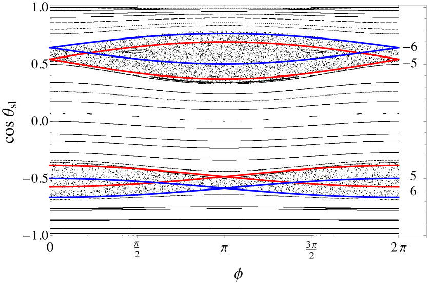
Figure 8: Surfaces of section for two pairs of resonances put together, with their respective analytically computed separatrices. Red: $N=5,\,M=-5$; blue: $N=6,\,M=-6$. The adiabaticity parameter is $\epsilon=0.1$.

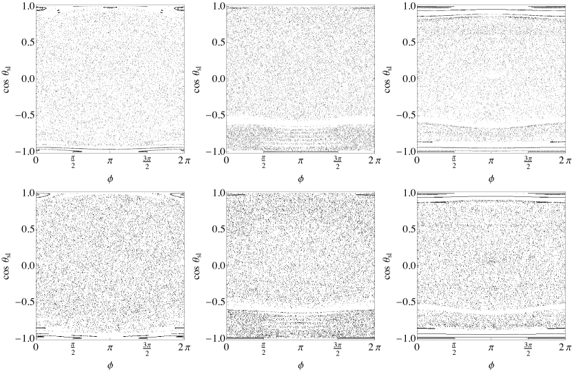
Figure 9: Surfaces of section computed using the exact Hamiltonian (top panels) and using the approximate Hamiltonian with only the $\{-N_{\rm max},N_{\rm max}\}$ Fourier harmonics included in the forcing function (bottom panels). The panels from left to right correspond to $\epsilon=0.1$, $0.05$, $0.02$. Note the agreement between top and bottom panels becomes better with smaller values of $\epsilon$.

Figure 7 illustrates the onset of chaos due to overlapping resonances. Note that the separatrix of each of these resonances is time-independent only in its own frame of reference. Thus, to visualize the combined effect of both resonances and be able to interpret them using resonance overlaps, we construct surfaces of section. Specifically, we record $p$ and $\phi$ only once per eccentricity cycle at $\tau=0,2\pi,4\pi,\cdots$, because in this case we have $H(\bar{\phi})=H(\phi)$ for any harmonic. This enables us to overlay analytic calculations of the separatrices on top of the surface of section in a meaningful way. By doing this, we can say that Figure 7 indeed demonstrates that, approximately, given two resonances $N$ and $M$ separated by a distance $\Delta p$, chaotic evolution of $p=\cos\theta_{\rm{sl}}$ is induced when

$$\Delta p\mathrel{\raise 1.29167pt\hbox{$<$}\mkern-14.0mu\lower 2.58334pt\hbox{$\sim$}}\frac{1}{2}\left(w_{N}+w_{M}\right).$$ (58)

When this occurs, the region of chaotic evolution approximately spans the areas of both separatrices.

Figure 8 shows an example when four resonances are included in the Hamiltonian. In practice, a particular resonance likely only overlaps with the resonance nearest to it. Thus it is possible to observe features such as those depicted in Figure 8: multiple isolated regions of chaos separated by a large domain of periodic space.

6 Application to the Full Problem of Lidov-Kozai driven Spin Precession

We now examine the full problem of stellar spin dynamics driven by a planet undergoing LK cycles, with the Hamiltonian given by Eq. (37). If the chaotic behaviour of this full system is indeed determined by resonances and their overlaps, and, as discussed in Section 3.3, there exists a maximum resonance order $N_{\rm max}$, we expect that approximating this full system with one consisting only of all harmonics with $|N|<N_{\rm max}$ should reproduce the key features of the system. Thus we consider the approximate Hamiltonian

$$H^{\prime}_{\rm app}\simeq\frac{\bar{\alpha}}{n_{e}}\biggl{[}-\frac{1}{2}p^{2}+\epsilon\,\psi_{0}\,p$$

$$\qquad-\frac{\epsilon}{2}\sqrt{1-p^{2}}\!\!\sum_{N=-N_{\rm max}}^{N_{\rm max}}\!\!\!\left(\beta_{N}+\gamma_{N}\right)\cos(\phi-N\tau)\biggr{]}.$$ (59)

We evolve equations of motion obtained from both Eq. (37) and Eq. (59). Figure 9 compares the resulting surfaces of section for several values of $\epsilon$. It is apparent that taking only the innermost $2N_{\rm max}+1$ harmonics in the perturbing functions adequately reproduces the behavior of the full system, with better agreement for smaller $\epsilon$.

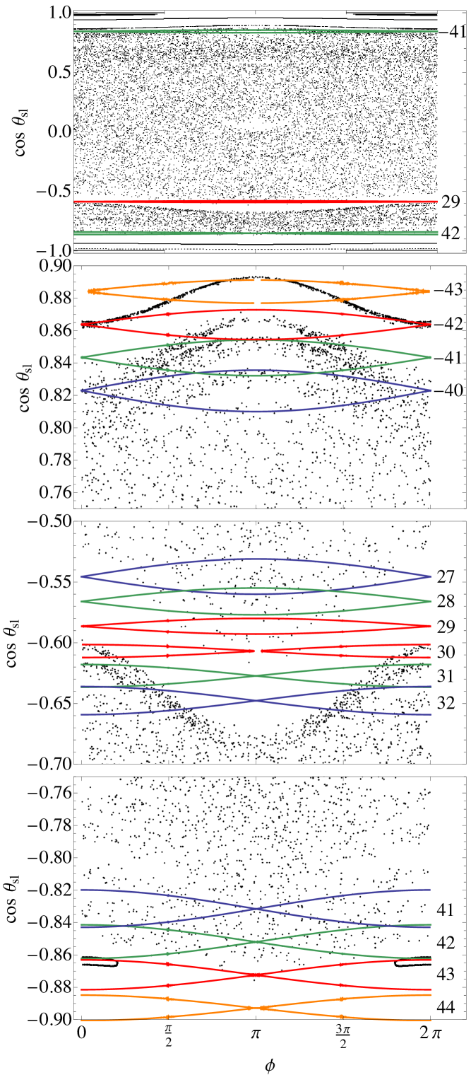
Figure 10: Demonstration of how overlapping resonances can explain several features of the $\epsilon=0.02$ surface of section shown in the right panels of Fig. 9. Top panel : The entire surface of section, with the separatrices for the N=$42$ (bottom green), $29$ (red), and $-41$ (top green) resonances overlaid. Second panel : Zoom-in on the top portion of the surface of section; the separatrices for resonances with $N=-40$ (blue), $-41$ (green), $-42$ (red), and $-43$ (orange) are overlaid. Third panel : Zoom-in on the gap located at $p\approx-0.6$; from top to bottom, the separatrices for the $N=27$ (blue), $28$ (green), $29$ (red), $30$ (red), $31$ (green), and $32$ (blue) resonances are overlaid. Bottom panel : Zoom-in on the bottom portion of the surface of section; the separatrices for $N=41$ (blue), $42$ (green), $43$ (red), and $44$ (orange) are overlaid.

We may now consider whether the overlap of these resonances can explain the width of the chaotic region as a function of $\epsilon$. Figure 10 shows that this is indeed the case. Given a value of $\epsilon$, there exists a positive “outermost” resonance $N=N^{+}_{\rm out}$ ($>0$) which overlaps with the “previous” resonance ($N^{+}_{\rm out}-1$) but not with the “next” one ($N^{+}_{\rm out}+1$). Since the separation (in $p$) of two neighboring resonances is $\Delta p\simeq 1/N_{\rm max}$ [see Eq. (48)], this “outermost” resonance is determined by the conditions

$${1\over 2}\left(w_{N^{+}_{\rm out}}+w_{N^{+}_{\rm out}-1}\right)>{1\over N_{\rm max}},$$ (60)

and

$${1\over 2}\left(w_{N^{+}_{\rm out}}+w_{N^{+}_{\rm out}+1}\right)<{1\over N_{\rm max}}.$$ (61)

Likewise, there exists a negative “outermost” resonance $N^{-}_{\rm out}$ ($<0$) which is the last to overlap with the “previous” one ($N^{-}_{\rm out}+1$). The locations of these two “outermost” resonances, as determined by the resonant momenta $p^{\pm}_{\rm N,out}\simeq-N^{\pm}_{\rm out}/N_{\rm max}$, bound the chaotic region in the $p$-space .

As $\epsilon$ is varied, $N^{\pm}_{\rm out}$ and $p^{\pm}_{\rm N,out}$ vary as well. Thus we may analytically compute the extent (i.e. the outermost boundaries in the $p$-space) of wide-spread chaos as a function of $\epsilon$. The result is shown in Figure 11 (note that winthin the chaotic zone in $p$-space, there can still exist periodic islands; see below).

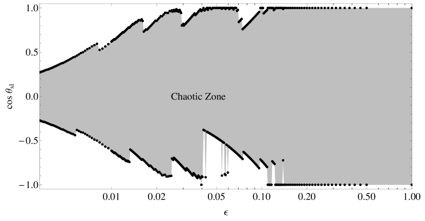
Figure 11: Outermost boundaries of the chaotic region as a function of $\epsilon$, calculated by determining the outermost resonance $N^{\pm}_{\rm out}$ which still overlaps with the previous one. The non-monotonic nature of the width of the chaotic region is due to the non-monotonic behavior of the Fourier coefficients of the resonant forcing terms ($\beta_{N}+\gamma_{N}$; see Fig. 3). Note that while the spin evolution is strictly non-chaotic outside the chaotic zone (the shaded region), there could be periodic windows inside the chaotic zone.

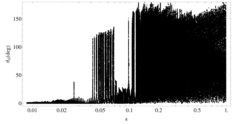
Figure 12: “Bifurcation” diagram of spin-orbit misalignment angle versus the adiabaticity parameter $\epsilon$. For each $\epsilon$, we evolve the equations of motion starting with $\theta_{\rm{sl}}=0$, for $\sim\!500$ LK orbital eccentricity cycles, and record $\theta_{\rm{sl}}$ every time the eccentricity reaches a minimum. This diagram is similar to Fig. 1, except that all short-range force effects and the back-reaction of the stellar spin on the orbit are turned off.

Figure 10 brings to light another interesting feature of this dynamical system: the existence of narrow regions of non-chaotic behavior, spanning the entire $\{0,2\pi\}$ range in the $\phi$ coordinate and thus effectively splitting the phase space into chaotic regions that cannot communicate with each other. This feature arises from the strongly nonlinear variation of the Fourier coefficient ($\beta_{N}+\gamma_{N}$), and therefore the widths, of the various resonances involved: resonances that are very narrow are isolated from the surrounding ones, and quasiperiodic behavior becomes possible in their vicinity. For example, from Figure 5 we see that for $\epsilon=0.05$, the resonances of order $N=11$ and $12$ are particularly narrow, and indeed they are the ones that cause the narrow band in the middle panels of Fig. 9. Likewise, as demonstrated in the third panel of Fig. 10, for $\epsilon=0.02$, the resonances $N=29$ and $30$ are isolated from the rest and result in a band of quasi-periodicity.

We now focus on systems which start out with aligned stellar spin and planetary angular momentum axes (i.e. $\cos\theta_{\rm{sl}}=1$) – such systems are very relevant in the standard picture where planets form in protoplanetary disks aligned with the central stars. Two questions are of interest: first, given a specific value of $\epsilon$, will such an initially aligned state experience chaotic or quasiperiodic evolution, and second, if the evolution is chaotic, how much of the available phase space will it span, i.e. how much will $\cos\theta_{\rm{sl}}$ vary? (A third question may also be asked - what happens if $\epsilon$ slowly evolves as a function of time, as it might in a physical system due to tidal dissipation? We address this issue in Section 7 below).

To address these questions, we numerically construct a “bifurcation diagram” (Fig. 12), using the equations of motion of the full Hamiltonian (Eq. 37). For each value of $\epsilon$ we compute the spin evolution trajectory starting from the initial condition $\cos\theta_{\rm{sl}}=1$. We record on the $y$-axis the spin-orbit misalignment angle at every eccentricity minimum (at $\tau=0,2\pi,4\pi$…). The result is, effectively, a 1D surface of section, for a single initial condition. We then repeat the calculation for a fine grid of $\epsilon$ values. Figure 12 shows the result. Large spread in $\theta_{\rm{sl}}$ indicates chaotic behavior, while small spread with well-defined edges indicates quasiperiodicity. We see from Fig. 12 that, in general, the spread of $\theta_{\rm{sl}}$ as a function of $\epsilon$ follows the trend analytically predicted in Fig. 11. For example, Figure 11 shows that for $\epsilon\mathrel{\raise 1.29167pt\hbox{$>$}\mkern-14.0mu\lower 2.58334pt\hbox{$\sim$}}0.1$, the spin-orbit misalignment of an initially aligned state will evolve chaotically; this is consistent with Fig. 12, which shows that $\theta_{\rm{sl}}$ undergoes large excusion for $\epsilon\mathrel{\raise 1.29167pt\hbox{$>$}\mkern-14.0mu\lower 2.58334pt\hbox{$\sim$}}0.1$. Figure 11 also shows that only for $\epsilon\mathrel{\raise 1.29167pt\hbox{$<$}\mkern-14.0mu\lower 2.58334pt\hbox{$\sim$}}0.02$, the aligned initial state will not evolve into the chaotic zone; this is also reflected in Fig. 12, where for $\epsilon\mathrel{\raise 1.29167pt\hbox{$<$}\mkern-14.0mu\lower 2.58334pt\hbox{$\sim$}}0.02$ the spread in $\theta_{\rm{sl}}$ is confined to a narrow region around $\theta_{\rm{sl}}=0$.

However, the transition between adiabatic evolution and chaotic evolution of stellar spin for an initially aligned state is fuzzy. As seen in Fig. 12, for $\epsilon$ between $\sim 0.02$ and $\sim 0.1$, the regular (periodic) regions (with small spread in $\theta_{\rm{sl}}$) are interspersed with the chaotic zones (with large spread in $\theta_{\rm{sl}}$). In particular, for $\epsilon\sim 0.04-0.07$, the spin evolution is mostly chaotic but with somewhat regularly spaced periodic regions – “periodic islands in an ocean of chaos” (see Fig. 13). Toward smaller $\epsilon$, the periodic islands expand and the chaotic regions shrink, so that for $\epsilon\mathrel{\raise 1.29167pt\hbox{$<$}\mkern-14.0mu\lower 2.58334pt\hbox{$\sim$}}0.04$ the spin evolution becomes mostly periodic, with small finely tuned chaotic domains that are shown in Fig. 14 to be linearly spaced in $1/\epsilon$ – “chaotic zones in a calm sea”. To illustrate how the theory of overlapping resonances can explain these features, Figure 15 takes a closer look at the resonances near $\cos\theta_{\rm{sl}}=1$ for three closely spaced values of $\epsilon$. Naturally, as discussed in Section 3.3, the resonance that determines the evolutionary behavior of the initially-aligned system is $N=-N_{\rm max}$, since it has $p_{N}\simeq 1$. As $\epsilon$ is varied, the trajectory of the system falls either inside the $N=-N_{\rm max}$ resonance, or outside it, or right on its separatrix. The proximity of the $N=-N_{\rm max}$ resonance to the $N=-N_{\rm max}+1$ resonance then determines the evolutionary trajectory of the system. If the two resonances overlap strongly, then all trajectories in the vicinity will be chaotic, but this is not the case in Fig. 15. Instead, for small values of $\epsilon$, the $N=-N_{\rm max}$ separatrix appears to be close to, but not quite touching, its neighbor. This, in principle, does not completely preclude chaos, since the Chirikov criterion is, in fact, too strict and chaos can still exist when two resonances are sufficiently close to each other and the trajectories are close to one of the separatrices (Chirikov 1979; Lichtenberg & Lieberman 1992). This is the case in Fig. 15: the chaotic trajectory of the middle panel falls right on the separatrix and effectively “rides” it out and onto the neighboring resonance. Thus, the series of peaks at small values of $\epsilon$ in Fig. 12 are due to the varying proximity of the $N=-N_{\rm max}$ resonance to $\cos\theta_{\rm{sl}}=1$ and to its neighboring resonances.

7 Adiabatic Resonance Advection

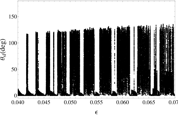
Figure 13: Zoom in on Fig. 12 in the region $0.04<\epsilon<0.07$. Here the spin evolution is mostly chaotic (with large scatter in $\theta_{\rm{sl}}$), with periodic regions (with $\theta_{\rm{sl}}$ close to zero) appearing in the middle of the chaos. The range of chaotic excursion is limited to be less than $\sim 130^{\circ}$ due to a periodic island at $\cos\theta_{\rm{sl}}\sim-0.5$ caused by the narrow width of the $N=11$ and $12$ resonances (see Fig. 5 and middle panels of Fig. 9).

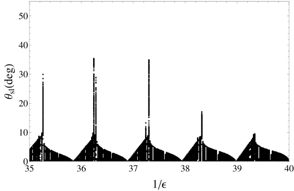
Figure 14: Zoom in on Fig. 12 in the region $0.025<\epsilon<0.0286$, plotted against $1/\epsilon$. Here the spin evolution is mostly regular or periodic (with small scatter in $\theta_{\rm{sl}}$), but chaotic zones (with large scatter in $\theta_{\rm{sl}}$) appear in the middle of the “calm sea”. The occurrence of the chaotic zones is approximately evenly spaced in $1/\epsilon$.

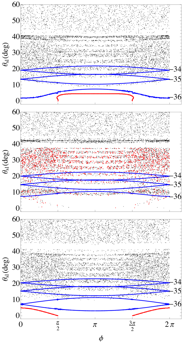
Figure 15: Demonstration of how the variation of resonances with $\epsilon$ leads to the peculiar oscillatory behavior seen in Fig. 14. The evolution of an initially aligned system is shown in red, and the analytical resonance separatrices are shown in blue. Top panel:  $1/\epsilon=37.1$; the initially aligned system is trapped within the $N=-36$ resonance, which is sufficiently far removed from the $N=-35$ resonance, so the trajectory is non-chaotic. Middle panel:  $1/\epsilon=37.3$; the $N=-36$ and $N=-35$ resonances are close, so the trajectory becomes chaotic; $\theta_{\rm{sl}}$ is confined to $<35^{\circ}$ because of the gap which separates the two chaotic zones. Bottom panel:  $1/\epsilon=37.4$; the $N=-36$ resonance has moved up sufficiently so that it no longer traps the initially aligned system, and the trajectory is regular again.

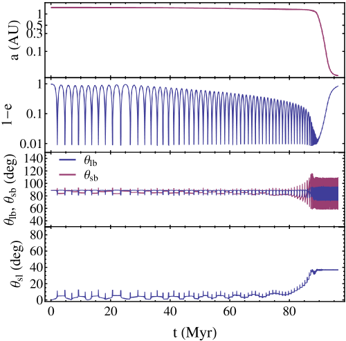
Figure 16: Sample time evolution demonstrating non-chaotic drift of an initially aligned system toward higher misalignment angles. The top panel shows the orbital semi-major axis, the second panel shows the eccentricity, the third panel shows the orbital inclination angle $\theta_{\rm lb}$ and the angle $\theta_{\rm sb}$ between $\hat{{\bf S}}$ and $\hat{{\bf L}}_{b}$, and the bottom panel shows the spin-orbit misalignment angle $\theta_{\rm{sl}}$. The parameters are $M_{p}=5M_{J}$, $\hat{\Omega}_{\star}=0.05$, $a_{0}=1.5$AU, $a_{b}=200$AU, $\theta^{0}_{\rm lb}=89^{\circ}$, and we have included all short-range effects (cf. Fig. 1). See SAL for details.

For a non-dissipative system, the adiabaticity parameter $\epsilon$ is a constant. In the previous sections we have demonstrated that the dynamical behavior of the stellar spin axis for different values of $\epsilon$ can be understood using secular spin-orbit resonances. Here we discuss the phenomenon of “adiabatic resonance advection”, and demonstrate the importance of resonances when dissipation is introduced in our system.

As noted in Section 1, in the “Lidov-Kozai + tide” scenario for the formation of hot Jupiters (Wu & Murray 2003; Fabrycky & Tremaine 2007; Correia et al. 2011; Naoz et al. 2012; Petrovich 2014; SAL), tidal dissipation in the planet at periastron reduces the orbital energy, and leads to gradual decrease in the orbital semi-major axis and eccentricity. In this process, $\epsilon$ slowly decreases in time. In SAL, we have considered various sample evolutionary tracks and shown that the complex spin evolution can leave an imprint on the final spin-orbit misalignment angle. A more systematic study will be presented in a future paper (Anderson, Storch & Lai 2015).

In Fig. 16, we show a particular evolutionary track of our system, obtained by integrating the full equations of motion for the LK oscillations, including the effects of all short-range forces (General Relativity, distortion of the planet due to rotation and tide, and rotational bulge of the host star) and tidal dissipation in the planet (see SAL for details). In this example, the adiabatic parameter $\epsilon\simeq 0.17$ initially and decreases as the orbit decays. So the spin evolution is always in the non-chaotic, adiabatic regime. Interestingly, we see that as $a$ decreases, the initially aligned state gradually drifts toward a higher misalignment angle in a well-ordered manner.

To explain this intriguing behavior, we consider a simplified version of the problem, in which we gradually increase $\alpha_{0}$ (thereby decreasing $\epsilon$) while keeping the forcing due to the planet unchanged. If the evolution of $\epsilon$ is sufficiently gradual, then given an initial state there exists an adiabatic invariant that is conserved as $\epsilon$ changes:

$$J=\oint p\,d\phi,$$ (62)

where the integration covers a complete cycle in the $\phi$-space. This quantity is equivalent to the area enclosed by the trajectory in phase space. Since, as discussed previously, the $N=-N_{\rm max}$ resonance is the one that most strongly influences the initially-aligned system, we consider the single-resonance Hamiltonian (Eq. 53) for this resonance. Since this Hamiltonian is independent of time, it is conserved, i.e. $E=H(\phi_{0},p_{0})$ is a constant so long as $\epsilon$ is constant. Conversely, a single value of $E$ corresponds to a unique phase space trajectory $p(\phi;E,\epsilon)$. It follows that the adiabatic invariant can be expressed as a function of $E$ and $\epsilon$, i.e., $J=J(E,\epsilon)$.

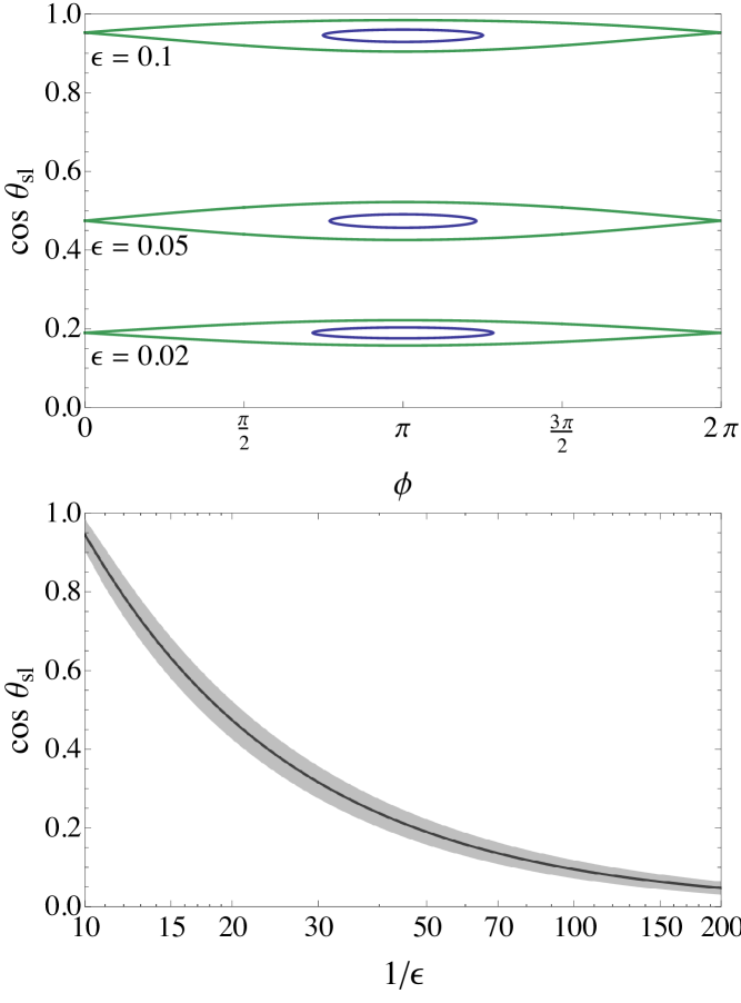
Figure 17: Proof of concept for “adiabatic resonance advection”. Top panel:  Sample spin evolution trajectories (constant-energy curves in the $\cos\theta_{\rm{sl}}$-$\phi$ phase space) for several values of $\epsilon$. The system initially has $\epsilon=0.1$ and is contained within the $N=-9$ resonance with $p_{N}\simeq 1$. As $\epsilon$ slowly decreases due to dissipation, the resonance center $p_{N}$ moves to smaller values, with the sample trajectory’s area remaining constant. Bottom panel:  Location (solid black line) and width (grey area) of the $N=-9$ resonance as a function of $1/\epsilon$, demonstrating that $p_{N}$ moves toward $p=0$ and the resonance width (in $\cos\theta_{\rm{sl}}$) narrows with decreasing $\epsilon$. The sample trajectory trapped inside the resonance must follow the resonance in accordance with the principle of adiabatic invariance.

As the system evolves ($\epsilon$ slowly changes), $J(E,\epsilon)$ is kept constant, so $E$ must change. These changes in $\epsilon$ and $E$ lead to changes in the phase space trajectory. For an initially circulating trajectory that spans the entire $\{0,2\pi\}$ range in $\phi$, to conserve the area under the curve the most that can happen is that an initially curved trajectory must flatten, approaching $p={\rm const}$, where the constant is roughly the average of $p$ over the initial trajectory. However, if a trajectory is librating and only encloses a small area, it can be a lot more mobile as $\epsilon$ evolves. As demonstrated in Fig. 15, one way for the initially-aligned trajectory to be librating is for it to be trapped inside the $-N_{\rm max}$ resonance. We also know that as $\epsilon$ decreases the resonance must move toward $p=0$ [see Eqs. (47)-(48)]. We therefore posit that it is possible that the initially-aligned trajectory can be advected with the resonance, and gradually taken to higher misalignment angles. A proof of concept of this process is shown in Fig. 17. While a detailed study of this process (such as the condition for resonance trapping) is beyond the scope of this paper, we note that it has many well-known parallels in other physical systems, such as the trapping of mean-motion resonances when multiple planets undergo convergent migration.

8 Conclusion

In this work we have continued our exploration of Lidov-Kozai driven chaotic stellar spin evolution, initially discussed in Storch, Anderson & Lai (2014), by developing a theoretical explanation for the onset of chaos in the “adiabatic” to “trans-adiabatic” regime transition. The behaviour of the stellar spin evolution depends on the adiabaticity parameter $\epsilon$ [see Eq. (1) or (24)]. Using Hamiltonian perturbation theory, we have identified a set of spin-orbit resonances [see Eq. (45)] that determine the dynamical behaviour of the system. The resonance condition is satisfied when the averaged spin precession frequency of the star is an integer multiple of the Lidov-Kozai precession frequency of the planet’s orbit. We have shown that overlaps of these resonances lead to the onset of chaos, and the degree of overlap determines how wide-spread the chaos is in phase space. Some key properties of the system include the facts that the width of an individual resonance is a non-monotonic function of the resonance order $N$ (see Fig. 5), and that there exists a maximum order $N_{\rm max}$ [see Eq. (47)] that influences the spin dynamics. These properties lead to several unusual features (such as “periodic islands in an ocean of chaos”) when the system transitions (as $\epsilon$ decreases) from the fully chaotic regime to the fully adiabatic regime (see Fig. 12). Focusing on the systems with zero initial spin-orbit misalignment angle, our theory fully predicts the region of chaotic spin evolution as a function of $\epsilon$ (see Fig. 11) and explains the non-trivial features found in the numerical bifurcation diagram (Fig. 12). Finally, we use the spin-orbit resonance and the principle of adiabatic invariance to explain the phenomenon of “adiabatic resonance advection”, in which the spin-orbit misalignment accumulates in a slow, non-chaotic way as $\epsilon$ gradually decreases as a result of dissipation (see Section 7).

The system we considered in this paper is idealized. We have not included the effects of short-range forces, such as periastron advances due to General Relativity, and the planet’s rotational bulge and tidal distortion. We have also ignored the back-reaction torque from the stellar quadrupole on the orbit. These simplifications have allowed us to focus on the spin dynamics with “pure” orbital Lidov-Kozai cycles. Finally, we have only briefly considered the effects of tidal dissipation, using an idealized model in which the “shape” of the Lidov-Kozai oscillations does not change as the semi-major axis decays. All of these effects will eventually need to be included, if we hope to not only understand the origin of the chaotic behavior but also make predictions for the observed spin-orbit misalignment distributions in hot Jupiter systems. We begin to systematically explore these issues numerically in a future paper (Anderson, Storch & Lai 2015).

References

- author (2000) Anderson, K.R., Storch, N.I., & Lai, D. 2015, in prep
- author (2000) Albrecht, S., et al. 2012, Astrophys. J. 757, 18
- author (2000) Bate, M. R., Lodato, G., & Pringle, J. E. 2010, MNRAS, 401, 1505
- author (2000) Batygin, K. 2012, Nature, 491 418
- author (2000) Batygin, K., & Adams, F. C. 2013, Astrophys. J. 778, 169
- author (2000) Chirikov, B. V. 1979, Phys. Rep. 52, 263
- author (2000) Correia, A. C. M., Laskar, J.,Farago, F., & Bou , G. 2011, Celest. Mech. Dynam. Astron. 111, 105
- author (2000) Fabrycky, D., & Tremaine, S. 2007, Astrophys. J. 669, 1298
- author (2000) Ford, E. B., Kozinsky, B., & Rasio, F. A. 2000, Astrophys. J. 535, 385
- author (2000) Hebrard, G., et al. 2008, A&A, 488, 763
- author (2000) H brard, G., et al. 2010 A&A 516, 95
- author (2000) Katz, B., Dong, S., & Malhotra, R. 2011, Phys. Rev. Lett. 107, 181101
- author (2000) Kinoshita, H. 1993, Celestial Mechanics and Dynamical Astronomy, 57, 359
- author (2000) Kinoshita, H. & Nakai, H. 1999, CeMDA, 75, 125
- author (2000) Kozai, Y. 1962, Astron. J. 67, 591
- author (2000) Lai, D. 2014, MNRAS 440, 3532
- author (2000) Lai, D., Foucart, & Lin, D. N. C. 2011, MNRAS 412, 2790
- author (2000) Laskar, J., Robutel, P. 1993, Nature, 361, 608
- author (2000) Li, G., & Batygin, K. 2014, ApJ, 790, 69
- author (2000) Li, G., Naoz, S., Holman, M., & Loeb, A. 2014, ApJ, 791, 96
- author (2000) Lichtenberg, A. & Lieberman, M. 1992, Regular and Chaotic Dynamics, ed. J.E. Marsden & L. Sirovich, Springer-Verlag, New York
- author (2000) Lidov, M. L. 1962, Planet. Space Sci. 9, 719
- author (2000) Liu., B., Munoz, D., & Lai, D. 2014, submitted (arXiv:1409.6717)
- author (2000) Naoz, S., Farr, W. M., Lithwick, Y., Rasio, F. A., & Teyssandier, J. 2011, Nature 473, 187
- author (2000) Naoz, S., Farr, W. M., & Rasio, F. A. 2012, Astrophys. J. 754, L36
- author (2000) Naoz, S., Farr, W. M., Lithwick, Y., Rasio, F. A., & Teyssandier, J. 2013, MNRAS 431, 2155
- author (2000) Narita, N., Sato, B., Hirano, T., & Tamura, M. 2009, Publ. Astron. Soc. Jpn. 61, L35
- author (2000) Petrovich, C. 2014, submitted (arXiv:1405.0280)
- author (2000) Spalding, C., & Batygin, K. 2014, ApJ, 790, 42
- author (2000) Storch, N.I., Anderson, K.R., & Lai, D. 2014, Science, 345 (6202), 1317-1321
- author (2000) Touma, J., Wisdom, J. 1993, Science, 259, 1294
- author (2000) Triaud, A., et al. 2010, A&A, 524, A25
- author (2000) Winn, J. N. et al. 2009, Astrophys. J. 703, L99
- author (2000) Wu, Y., & Murray, N. 2003, Astrophys. J. 589, 605