Quasi-Monte Carlo methods for Choquet integrals

Abstract

We propose numerical integration methods for Choquet integrals where the capacities are given by distortion functions of an underlying probability measure. It relies on the explicit representation of the integrals for step functions and can be seen as quasi-Monte Carlo methods in this framework. We give bounds on the approximation errors in terms of the modulus of continuity of the integrand and the star discrepancy.

Key words: Choquet integrals, quasi-Monte Carlo methods, risk measures.

AMS MSC 2010: 65D30, 28A25, 65C05.

In this paper, we are concerned with numerical integration for Choquet integrals

(1) $$\int f(U)dc_{\psi}:=\int_{0}^{\infty}c_{\psi}(f(U)>x)dx+\int_{-\infty}^{0}(c_{\psi}(f(U)>x)-1)dx$$

for continuous functions $f$ on $[0,1]^{d}$, where $U$ is a $[0,1]^{d}$-valued and uniformly distributed random variable on an atomless probability space $(\Omega,\mathcal{F},\mathbb{P})$, the function $\psi:[0,1]\to[0,1]$ is increasing and concave such that $\psi(0)=0$, $\psi(1)=1$, and $c_{\psi}$ is the submodular set function defined by $c_{\psi}(A)=\psi(\mathbb{P}(A))$, $A\in\mathcal{F}$. We refer to Denneberg [2] for the theory of Choquet integrals.

The capacities of the form $c_{\psi}(A)=\psi(\mathbb{P}(A))$ as above appear in financial risk management. In particular, the case $\psi(t)=\min(t,\lambda)/\lambda$, for some $\lambda\in(0,1)$, corresponds to the risk measure known as the average-value-at-risk, which is also called as the conditional value-at-risk or the expected shortfall in practice. We refer to Artzner et al. [1], McNeil et al. [4], and Föllmer and Schied [3] for details.

As for numerical integration, several techniques that are analogous to those for the linear integral have been studied in the literature. See, e.g., [4] for Monte Carlo methods, and Nakano [5] for optimal quantization methods. However, to the best of our knowledge, quasi-Monte Carlo methods have not been examined to Choquet integrals despite of its popularity.

To find a suitable quasi-Monte Carlo method for (1), let $\{u_{i}\}_{i=1}^{n}$ is a point set in $[0,1]^{d}$ and consider the simple random variable $U^{(n)}$ defined by

$$U^{(n)}=\sum_{i=1}^{n}u_{i}1_{A_{i}},$$

where $\{A_{i}\}_{i=1}^{n}\subset\mathcal{F}$ is a partition of $\Omega$ such that $\mathbb{P}(A_{i})=1/n$, $i=1,\ldots,n$. Note that such $A_{i}$’s exist since $(\Omega,\mathcal{F},\mathbb{P})$ is assumed to be atomless. If $\{u_{i}\}$ is uniformly distributed, then we expect

$$\int f(U)dc_{\psi}\approx\int f(U^{(n)})dc_{\psi}.$$

Next, recall that the Choquet integral has the comonotonicity, i.e., for any random variables $X$ and $Y$ that are integrable with respect to $c_{\psi}$, we have

$$\int(X+Y)dc_{\psi}=\int Xdc_{\psi}+\int Ydc_{\psi}$$

whenever

(2) $$(X(\omega)-X(\omega^{\prime}))(Y(\omega)-Y(\omega^{\prime}))\geq 0$$

for all $(\omega,\omega^{\prime})\in\Omega\times\Omega$ except for a set of probability zero. Two random variables $X$ and $Y$ are said to be comonotone if they satisfy (2).

Now observe that for $A,B\in\mathcal{F}$, the two indicator functions $1_{A}$ and $1_{B}$ are comonotone if $A\supset B$. Thus, for $A_{i}\in\mathcal{F}$ and $a_{i}\in\mathbb{R}$, $i=1,\ldots,n$, we have

(3) $$\int\sum_{i=1}^{n}a_{i}1_{A_{i}}dc_{\psi}=\sum_{i=1}^{n}a_{i}\int 1_{A_{i}}dc_{\psi}$$

provided that $A_{1}\subset\cdots\subset A_{n}$ and $a_{i}\geq 0$, $i=1,\ldots,n$.

Let $\tau:\{1,\ldots,n\}\to\{1,\ldots,n\}$ be such that $f(u_{\tau(1)})\leq\cdots\leq f(u_{\tau(n)})$. Then we have the representation of $f(U^{(n)})$ given by

$$f(U^{(n)})=\sum_{i=1}^{n}f(u_{\tau(i)})1_{A_{\tau(i)}}=f(u_{\tau(1)})+\sum_{i=2}^{n}(f(u_{\tau(i)})-f(u_{\tau(i-1)}))1_{\cup_{k=i}^{n}A_{\tau(k)}}.$$

Applying this representation to (3), we obtain

$$\int f(U^{n})dc_{\varphi}=f(u_{\tau(1)})+\sum_{i=2}^{n}(f(u_{\tau(i)})-f(u_{\tau(i-1)}))c_{\psi}\left(\bigcup_{k=i}^{n}A_{\tau(k)}\right).$$

Consequently, since $c_{\psi}(\cup_{k=i}^{n}A_{\tau(k)})=\psi(\sum_{k=i}^{n}\mathbb{P}(A_{\tau(k)}))=\psi((n-i+1)/n)$, the quantity

$$I^{(n)}(f):=f(u_{\tau(1)})+\sum_{i=2}^{n}(f(u_{\tau(i)})-f(u_{\tau(i-1)}))\psi\left(\frac{n-i+1}{n}\right)$$

can be an approximation of $\int f(U)dc_{\psi}$.

To obtain an error bound, we use the star discrepancy $D^{*}(x_{1},\ldots,x_{m})$ defined by

$$D^{*}(x_{1},\ldots,x_{m})=\sup\left\{\frac{1}{m}\sum_{j=1}^{m}\left|1_{B}(x_{j})-\mathrm{Leb}(B)\right|\>:\>B=\prod_{i=1}^{d}[0,\xi_{i}),\;\xi_{k}\in[0,1],\;k=1,\ldots,d\right\}$$

for a point set $\{x_{i}\}_{i=1}^{m}\subset[0,1]^{d}$, where $\mathrm{Leb}$ stands for the Lebesgue measure on $[0,1]^{d}$. We refer to Niederreiter [6] for the relation between the discrepancy and numerical integration. Further, let $\rho(g;t)$ be the modulus of continuity of a function $g$ defined by

$$\rho(g;t)=\sup\{|g(x)-g(y)|:|x-y|\leq t,\;x,y\in[0,1]^{d}\},\quad t\geq 0,$$

where $|x|$ denotes the max norm of a vector $x$. Also, notice that by the concavity of $\psi$, the limit

$$\psi_{+}^{\prime}(t):=\lim_{s\searrow t}\frac{\psi(s)-\psi(t)}{s-t},\quad t\in[0,1),$$

exists for any $t\in[0,1)$ and decreasing with respect to $t$.

Then we have the following:

Theorem 1.

Under the assumptions and notations above, if $\rho(f;D^{*}(u_{1},\ldots,u_{n})^{1/d})<1$, we have

$$\left|\int f(U)dc_{\varphi}-I^{(n)}(f)\right|\leq\left(2\max_{u\in[0,1]^{d}}|f(u)|+4\right)\psi(\rho(f;D^{*}(u_{1},\ldots,u_{n})^{1/d})).$$

Moreover, if $\psi_{+}^{\prime}(0)<\infty$, then

$$\left|\int f(U)dc_{\varphi}-I^{(n)}(f)\right|\leq 4\psi_{+}^{\prime}(0)\rho(f;D^{*}(u_{1},\ldots,u_{n})^{1/d}).$$

Remark 2.

Since we have assumed that $f$ and $\psi$ are continuous with $\psi(0)=0$, the quantity $\psi(\rho(f;D^{*}(u_{1},\ldots,u_{n})^{1/d}))$ and so the approximation error converge to zero, provided that $D^{*}(u_{1},\ldots,u_{n})\to 0$ as $n\to\infty$. In particular, if $\psi^{\prime}_{+}(0)<\infty$, the function $f$ is Lipschitz on $[0,1]^{d}$, and $\{u_{i}\}_{i=1}^{n}$ is a low-discrepancy point set, i.e., it satisfies

$$D^{*}(u_{1},\ldots,u_{n})\leq C\frac{(\log n)^{d}}{n}$$

for some positive constant $C$, then the theorem implies

$$\left|\int f(U)dc_{\varphi}-I^{(n)}(f)\right|\leq 4\psi_{+}^{\prime}(0)|f|_{Lip}C^{1/d}\frac{\log n}{n^{1/d}},$$

where $|f|_{Lip}$ is the Lipschitz constant of $f$.

Remark 3.

In case $\psi(t)=\min(t,\lambda)/\lambda$, we have $\psi_{+}^{\prime}(0)=1/\lambda<\infty$.

Remark 4.

If $d=1$ then the constant $4$ in the statement of the theorem is replaced by $1$. This can be verified from the proof below and Theorem 2.10 in [6].

Proof of Theorem 1.

By Lemma 4.63 in [3] we define the Borel probability measure $\mu$ on $[0,1]$ by the identity

$$\psi_{+}^{\prime}(t)=\int_{(t,1]}\frac{1}{s}\mu(ds),\quad t\in(0,1).$$

Then, from Lemma 4.46 and Theorem 4.64 in [3] it follows that

(4) $$\int Xdc_{\psi}=\int_{[0,1]}\frac{1}{\lambda}\inf_{y\in\mathbb{R}}\left(\mathbb{E}(X-y)_{+}+\lambda y\right)\mu(d\lambda)$$

for any bounded random variable $X$, where $(x)_{+}=\max(x,0)$ for $x\in\mathbb{R}$. Moreover, for each $\lambda\in(0,1)$, the infimum of the integrand in (4) is attained by

$$y_{X}(\lambda):=\inf\{x\in\mathbb{R}:\mathbb{P}(X>x)\leq\lambda\}.$$

Writing (4) with $X=f(U),f(U^{(n)})$, we have for $\varepsilon\in[0,1)$,

$$\int f(U)dc_{\psi}-\int f(U^{(n)})dc_{\psi}$$

$$\leq\int_{[0,\varepsilon]}\bigg{\{}\frac{1}{\lambda}\mathbb{E}[(f(U)-y_{f(U^{(n)})}(\lambda))_{+}+\lambda y_{f(U^{(n)})}(\lambda)]-\frac{1}{\lambda}\mathbb{E}[(f(U^{(n)})-y_{f(U^{(n)})}(\lambda))_{+}+\lambda y_{f(U^{(n)})}(\lambda)]\bigg{\}}\mu(d\lambda)$$

$$\quad+\int_{(\varepsilon,1]}\bigg{\{}\frac{1}{\lambda}\mathbb{E}[(f(U)-y_{f(U^{(n)})}(\lambda))_{+}+\lambda y_{f(U^{(n)})}(\lambda)]-\frac{1}{\lambda}\mathbb{E}[(f(U^{(n)})-y_{f(U^{(n)})}(\lambda))_{+}+\lambda y_{f(U^{(n)})}(\lambda)]\bigg{\}}\mu(d\lambda).$$

Since $\inf_{y\in\mathbb{R}}((a-y)_{+}+\lambda y)=\lambda a$, $a\in\mathbb{R}$, the first term in the equality just above is at most $2\max_{u\in[0,1]^{d}}|f(u)|\mu([0,\varepsilon])$. By Fubini’s theorem, the second term is equal to

(5) $$\int_{[0,1]^{d}}F^{(n)}(u)du-\frac{1}{n}\sum_{j=1}^{n}F^{(n)}(u_{i}),$$

where

$$F^{(n)}(u)=\int_{(\varepsilon,1]}\frac{1}{\lambda}(f(u)-y_{f(U^{(n)})}(\lambda))_{+}\mu(d\lambda).$$

By Theorem 1 in Proinov [7], the quantity (5) is bounded by $4\rho(F^{(n)};D^{*}(u_{1},\ldots,u_{n})^{1/d})$. Furthermore, it is straightforward to see that $\rho(F^{(n)};t)\leq\psi_{+}^{\prime}(\varepsilon)\rho(f;t)$. Summarizing the above arguments, we deduce that

$$\int f(U)dc_{\psi}-\int f(U^{(n)})dc_{\psi}\leq 2\max_{u\in[0,1]^{d}}|f(u)|\mu([0,\varepsilon])+4\psi_{+}^{\prime}(\varepsilon)\rho(f;D^{*}(u_{1},\ldots,u_{n})^{1/d}).$$

A similar argument shows that $\int f(U^{(n)})dc_{\psi}-\int f(U)dc_{\psi}$ is bounded by the right-hand side in the inequality just above. Thus,

(6) $$\left|\int f(U)dc_{\psi}-I^{(n)}(f)\right|\leq 2\max_{u\in[0,1]^{d}}|f(u)|\mu([0,\varepsilon])+4\psi_{+}^{\prime}(\varepsilon)\rho(f;D^{*}(u_{1},\ldots,u_{n})^{1/d}).$$

Now, if $\psi_{+}^{\prime}(0)<\infty$, then we set $\varepsilon=0$ in (6) to obtain the second assertion of the theorem. Otherwise, we use an argument from the proof of Lemma 4.63 in [3] to obtain $\mu([0,\varepsilon])=\psi(\varepsilon)-\varepsilon\psi_{+}^{\prime}(\varepsilon)\geq 0$. Therefore, by the choice $\varepsilon=\rho(f;D^{*}(u_{1},\ldots,u_{n})^{1/d})$ the right-hand side in (6) is estimated as

$$2\max_{u\in[0,1]^{d}}|f(u)|\psi(\rho(f;D^{*}(u_{1},\ldots,u_{n})^{1/d}))+4\psi(\rho(f;D^{*}(u_{1},\ldots,u_{n})^{1/d})).$$

Thus the first assertion of the theorem follows. ∎

Example 5.

Here, we present a numerical result in the case of $\psi(t)=\min(t,0.05)/0.05$, $t\in[0,1]$, and

$$f(u)=\exp\left[-\left\{u^{1}u^{2}u^{3}+\sin(u^{3}u^{4}u^{5})\right\}\right],\quad u=(u^{1},u^{2},u^{3},u^{4},u^{5})\in[0,1]^{5}.$$

We use the Halton sequence to compute $Q^{(n)}$. As a comparison, we take the Monte Carlo method, which is described by

$$I_{M}^{(n)}(f):=f(U_{\sigma(1)})+\sum_{i=2}^{n}(f(U_{\sigma(i)})-f(U_{\sigma(i-1)}))\psi\left(\frac{n-i+1}{n}\right),$$

where $\{U_{n}\}_{n=1}^{\infty}$ is an IID sequence with uniform distribution on $[0,1]^{5}$ and $\sigma:\{1,\ldots,n\}\to\{1,\ldots,n\}$ is such that $f(U_{\sigma(1)})\leq\cdots\leq f(U_{\sigma(n)})$. Figure 1 plots values of $I^{(n)}(f)$ and $I_{M}^{(n)}(f)$ for $n$ from $10^{6}$ to $7\times 10^{6}$ with step $2\times 10^{5}$. We can see that $I^{(n)}(f)$ steadily approaches to a true value as $n$ increases, whereas the behavior of $I_{M}^{(n)}(f)$ is still volatile even for $n$ larger than $4\times 10^{6}$.

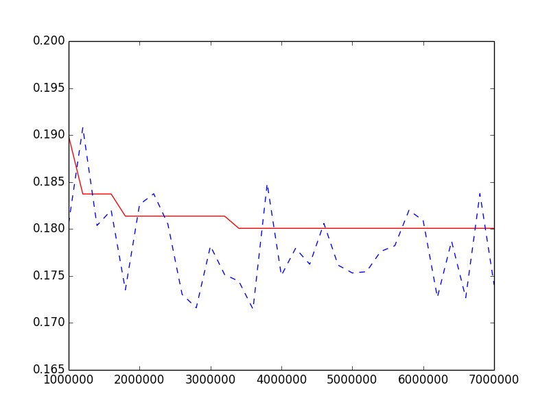
Figure 1: Nurimerical integrations of $f(U)$ with quasi-Monte Carlo (solid) and Monte Carlo (dashed) methods for $n$ from $10^{6}$ to $7\times 10^{6}$.

References

[1]
P. Artzner, F. Delbaen, J.-M. Eber, and D. Heath.
Coherent measurement of risk.
Math. Finance, 9:203–228, 1999.
[2]
D. Denneberg.
Non-additive measure and integral.
Kluwer Academic Publishers, Dordrecht, 1994.
[3]
H. Föllmer and A. Schied.
Stochastic Finance: An Introduction in Discrete Time.
Walter de Gruyter, Berlin, 2nd edition, 2004.
[4]
A. J. McNeil, R. Frey, and P. Embrechts.
Quantitative risk management: concepts, techniques and tools.
Princeton University Press, Princeton, 2005.
[5]
Y. Nakano.
On approximating law-invariant comonotonic coherent risk measures.
Astin Bulletin, 42:343–353, 2012.
[6]
H. Niederreiter.
Random number generation and quasi-Monte Carlo methods.
Society for Industrial and Applied Mathematics, Philadelphia, 1992.
[7]
P. D. Proinov.
Discrepancy and integration of continuous functions.
J. Approx. Theory, 52:121–131, 1988.