DESY 14-205
Multiple hard scattering and parton correlations in the proton

Abstract

This proceedings contribution gives a brief introduction to the theoretical description of double parton scattering and discusses several open problems.

1 Introduction

The standard description of hard processes in proton-proton (and other hadron-hadron) collisions uses the concept of factorization. In a standard factorization formula, the proton-proton cross section is given by the convolution of a parton density for each proton with a hard cross section for the interaction of two partons, summed over the relevant combinations of parton species. The physical picture suggested by this formula, represented in the left panel of Fig. 1, is deceptively simple since it suggests that the only interaction taking place in the collision is between the two partons initiating the hard subprocess. This is certainly not the case: the “spectator partons” in each proton are colored and will interact with their counterparts in the other proton, as sketched in the right panel of Fig. 1.

   

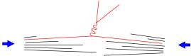
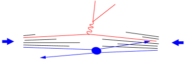
Figure 1: Sketch for the production and decay of a heavy gauge boson ($Z,W$ or off-shell $\gamma^{*}$) in a $pp$ collision. The left panel shows the picture suggested by the standard factorization formula for this process, whereas the right panel includes scattering between “spectator partons” that do not participate in the gauge boson production subprocess.

To solve this apparent contradiction, we first note that the factorization formula describes semi-inclusive processes of the type $pp\to Y+X$. Here $Y$ is the set of particles produced by the hard scattering (a lepton pair in Fig. 1), whereas $X$ denotes all other final-state particles. One can specify all details of $Y$ (and compute them from the hard scattering) but must sum over all possible hadronic states in $X$. The “spectator” interactions just mentioned affect particles in $X$, and it is a non-trivial statement of the factorization formula that—thanks to unitarity—one can ignore these interactions when computing the inclusive cross section $\sum_{X}\sigma(pp\to Y+X)$.

At the high collision energies of the LHC and the Tevatron, “spectator” interactions can themselves be hard and produce particles with large mass or large transverse momentum. For many purposes it is then not sufficient to known only $\sum_{X}\sigma(pp\to Y+X)$, and one is interested in the details of $X$. Recall that many search channels for new particles have high multiplicity due to long decay chains; in this case some of the relevant particles may belong to $Y$ but others to $X$. A sufficiently quantitative understanding of multiple hard interactions in $pp$ collisions is therefore important.

Even to understand double parton scattering, with two hard scatters as in the right panel of Fig. 1, remains a challenge for theory and phenomenology. Building on pioneering work done in the 1980s,[1, 2] we have in Refs. [Diehl:2011tt,Diehl:2011yj] shown that several aspects of double parton scattering allow for a systematic treatment in QCD, but that a number of open issues remain to be understood. This proceedings contribution presents a selection of theory results and of open questions.

2 Double scattering cross section

Let us assume that proton-proton collisions in which two pairs of partons initiate two independent hard-scattering processes can be described by a factorization formula akin to the familiar one for single hard scattering. The bound-state structure of each proton is then described by double parton distributions, i.e. by the joint distributions of the two scattering partons inside a proton. A corresponding graph is shown in Fig. 2.

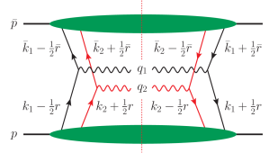
Figure 2: Graph for the production of two gauge bosons (with momenta $q_{1}$ and $q_{2}$) by two independent hard-scattering processes. Double parton distributions are represented by the blobs. The graph is for the inclusive cross section, with the final-state cut indicated by a dotted vertical line. Using momentum conservation one easily finds $r+\bar{r}=0$ for the momentum mismatch between partons on the left and the right of the cut.

A simple kinematic analysis shows that the plus- and minus-momentum components of each parton in the graph are fixed by the observable gauge boson momenta, because the partons in one proton carry only large plus-momentum and those in the other proton only large minus-momentum. By contrast, all partons generically carry transverse momenta of similar size. As a consequence, the partons that produce a given boson can have different transverse momenta in the scattering amplitude and in its conjugate, and the cross section formula involves a transverse-momentum convolution even if the transverse momenta of the gauge bosons are integrated over. In that case, the factorization formula can be written as

$$\frac{d\sigma_{\text{double}}}{dx_{1}\mskip 1.5mud\bar{x}_{1}\,dx_{2}\mskip 1.5mud\bar{x}_{2}} =\frac{1}{C}\,\hat{\sigma}_{1}\mskip 1.5mu\hat{\sigma}_{2}\int\frac{d^{2}\boldsymbol{r}}{(2\pi)^{2}}\;F(x_{1},x_{2},\boldsymbol{r})\,F(\bar{x}_{1},\bar{x}_{2},-\boldsymbol{r})\,,$$ (1)

where $C$ is a combinatorial factor and $\hat{\sigma}_{i}$ is a hard-subprocess cross section. $F(x_{1},x_{2},\boldsymbol{r})$ and $F(\bar{x}_{1},\bar{x}_{2},-\boldsymbol{r})$ are double parton distributions, whose $x$ arguments are fixed as $x_{i}=(\bar{p}\mskip 1.5muq_{i})/(\bar{p}\mskip 1.5mup)$ and $\bar{x}_{i}=(p\mskip 1.5muq_{i})/(p\mskip 1.5mu\bar{p})$. The formula is schematic in the sense that the quantum numbers of the partons have been omitted and that a sum over all relevant combinations should be taken. More detail can be found in Refs. [Diehl:2011tt,Diehl:2011yj].

Let us take the two-dimensional Fourier transform of $F(x_{1},x_{2},\boldsymbol{r})$ w.r.t. $\boldsymbol{r}$. The convolution integral in the cross section then becomes

$$\int\frac{d^{2}\boldsymbol{r}}{(2\pi)^{2}}\;F(x_{1},x_{2},\boldsymbol{r})\,F(\bar{x}_{1},\bar{x}_{2},-\boldsymbol{r}) =\int d^{2}\boldsymbol{y}\;F(x_{1},x_{2},\boldsymbol{y})\,F(\bar{x}_{1},\bar{x}_{2},\boldsymbol{y})\,.$$ (2)

The Fourier conjugate variable $\boldsymbol{y}$ can be interpreted as the transverse distance between the two partons with longitudinal momentum fractions $x_{1}$ and $x_{2}$, and hence as the transverse distance between the two hard-scattering processes.

The result (1) is a collinear factorization formula at tree level. It can readily be generalized to include higher orders in the subprocess cross sections $\hat{\sigma}_{i}$, which are identical to those calculated for single hard scattering. As in that case, the momentum arguments of the parton distributions are then no longer fixed in the cross section but appear in convolution integrals.

A different generalization of Eq. (1) is for measured transverse momenta $\boldsymbol{q}_{i}$ of the gauge bosons. If these are much smaller than the hard scale $Q$ of the scattering (i.e. if $\boldsymbol{q}_{i}^{2}\ll q_{i}^{2}$) one has a TMD-type factorization formula, with double parton distributions $F(x_{1},x_{2},\boldsymbol{k}_{1},\boldsymbol{k}_{2},\boldsymbol{r})$ and $F(\bar{x}_{1},\bar{x}_{2},\bar{\boldsymbol{k}}_{1},\bar{\boldsymbol{k}}_{2},-\boldsymbol{r})$ (see Fig. 2 for the momentum labeling). The partial Fourier transform $F(x_{1},x_{2},\boldsymbol{k}_{1},\boldsymbol{k}_{2},\boldsymbol{y})$ of $F(x_{1},x_{2},\boldsymbol{k}_{1},\boldsymbol{k}_{2},\boldsymbol{r})$ has the structure of a Wigner distribution in its transverse arguments: $\boldsymbol{k}_{1}$ and $\boldsymbol{k}_{2}$ are the transverse momenta of the two partons and $\boldsymbol{y}$ is their transverse distance if one “averages” over the two sides of the final-state cut, i.e. over the scattering amplitude and its conjugate.

The factorization formula (1) and its generalizations just discussed still have the status of conjectures: in Ref. [Diehl:2011yj] we could give several elements of a factorization proof, but several issues remain to be clarified and worked out. Perhaps the most serious one is the question whether soft gluon exchange between the spectator partons in the so-called Glauber region (where gluon momenta satisfy $l^{+}l^{-}\ll\boldsymbol{l}^{2}$) breaks factorization or not. The unitarity argument used for single gauge boson production cannot be readily generalized to double hard scattering, and it remains to be seen whether Glauber gluons invalidate the factorization formula (1).

3 Single vs. double hard scattering

A question of obvious concern is how important double hard scattering is compared with the conventional single hard scattering mechanism. The answer depends crucially on the observed kinematic variables in the final state. As indicated in Fig. 3, the double scattering mechanism is power suppressed by $\Lambda^{2}/Q^{2}$ w.r.t. single hard scattering in the collinear factorization formula, but it is not suppressed if the transverse boson momenta $\boldsymbol{q}_{1}$ and $\boldsymbol{q}_{2}$ are both measured. For small transverse momenta, $|\boldsymbol{q}_{i}|\ll Q$, both mechanisms are thus generically of the same size, whereas in the $\boldsymbol{q}_{i}$ integrated cross section single hard scattering wins because it populates a larger phase space with $|\boldsymbol{q}_{i}|\sim Q$, which is unaccessible to the double scattering mechanism.

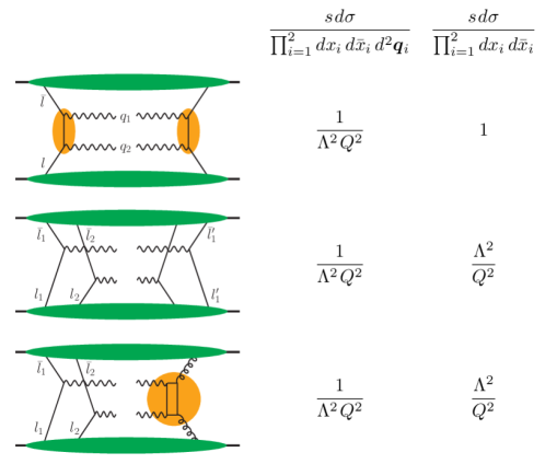
Figure 3: Example graphs and power behavior for the production of two gauge bosons by single hard scattering (top), double hard scattering (middle) and their interference (bottom). The shaded blobs indicate hard-scattering subprocesses. $\Lambda$ denotes a generic soft QCD scale, and $Q$ the hard scale of the scattering. The same power behavior is found for other final states.

At the same order in $\Lambda/Q$ as double hard scattering, there is also the interference between single and double scattering, shown in the bottom graph of Fig. 3. In this case, the hadronic quantities entering the collinear factorization formula are parton distributions of twist-three, where all parton fields are located at the same transverse position. This is in contrast to double scattering, where the partons associated with one or the other hard-scattering subprocess have a relative transverse distance $\boldsymbol{y}$ that is integrated over at the level of the cross section and not of the individual parton distributions. To our knowledge, such interference contributions have been ignored in phenomenological considerations so far, and nothing is known about their size in specific processes.

Apart from the hard scale $Q$, there is another parameter that controls the relative size of contributions in a generic manner, namely the overall $pp$ collision energy, which at given $Q$ translates into the typical size $x$ of the momentum fractions of the participating partons. Assuming the absence of correlations between small-$x$ partons, one finds that the cross sections for single and double parton scattering respectively scale like [4]

$$\frac{d\sigma_{\text{single}}}{dx_{1}\mskip 1.5mud\bar{x}_{1}\,dx_{2}\mskip 1.5mud\bar{x}_{2}} \sim\frac{1}{Q^{2}}\,x^{-4-2\lambda}\,, \frac{d\sigma_{\text{double}}}{dx_{1}\mskip 1.5mud\bar{x}_{1}\,dx_{2}\mskip 1.5mud\bar{x}_{2}} \sim\frac{\Lambda^{2}}{Q^{4}}\,x^{-4-4\lambda}$$ (3)

if the single-parton densities have a small-$x$ behavior $xf(x)\sim x^{-\lambda}$. Unless correlation effects overturn this trend, double parton scattering thus becomes enhanced at low $x$. A corresponding enhancement is also found if one considers gluon initiated hard-scattering processes and computes the energy dependence within the BFKL framework.[5] Unfortunately, not enough is known about the small-$x$ behavior of the three-parton correlation functions needed for the interference term in Fig. 3, so that it remains unclear whether it benefits from a similar low-$x$ enhancement.

4 Parton correlations

The double parton distributions $F(x_{1},x_{2},\boldsymbol{y})$ (and even more so their TMD counterparts) are barely known at present. As a zeroth-order approximation, one may assume the absence of correlations between the two partons and then obtains

$$F(x_{1},x_{2},\boldsymbol{y})\approx\int d^{2}\boldsymbol{b}\;f(x_{1},\boldsymbol{b}+\boldsymbol{y})\,f(x_{2},\boldsymbol{b})\,,$$ (4)

where $f(x,\boldsymbol{b})$ is the impact parameter distribution of a single parton,[6] i.e. the probability density for finding a parton with momentum fraction $x$ at a transverse distance $\boldsymbol{b}$ from the proton center. In transverse-momentum space, this relation is even simpler and reads [7]

$$F(x_{1},x_{2},\boldsymbol{r})\approx f(x_{1},\boldsymbol{r})\,f(x_{2},-\boldsymbol{r})\,,$$ (5)

where $f(x,\boldsymbol{r})$ is the Fourier transform of $f(x,\boldsymbol{b})$ w.r.t. $\boldsymbol{b}$.

Several arguments speak against the independence of the two partons expressed in (4) and (5) if the momentum fractions $x_{1}$ and $x_{2}$ are not very small. We will not go into details here but instead refer to Ref. [Diehl:2013mma]. Such correlations may concern only the overall size of $F(x_{1},x_{2},\boldsymbol{y})$, or depend only on the momentum variables $x_{1}$ and $x_{2}$, or correlate $x_{1}$ and $x_{2}$ with $\boldsymbol{y}$.

Moreover, the spin or the color of the two partons can be correlated. Such correlations can be quantified by polarization or color dependent distributions, which must be included in the factorization formula (1). For these distributions, a factorized form as in (4) and (5) is hardly plausible even as a starting point.

Correlations between $x_{1},x_{2}$ and $\boldsymbol{y}$ can have important quantitative consequences on double scattering cross sections,[9] and the same is true for parton spin correlations.[10] Color correlations are suppressed by Sudakov factors in the collinear factorization formula,[11, 4, 12] but according to the estimate in Ref. [Manohar:2012jr] this suppression is not very strong for moderately high scales.

5 Short-distance behavior, evolution and an unsolved problem

Using power counting arguments, one can show that for $|\boldsymbol{y}|\ll 1/\Lambda$ the distributions $F(x_{1},x_{2},\boldsymbol{y})$ can be computed in terms of single parton densities and a hard-scattering kernel $K$ that describes the splitting of one parton into two.[4] An example is shown in the left panel of Fig. 4. At lowest order in $\alpha_{s}$ one then has [4]

$$F(x_{1},x_{2},\boldsymbol{y})=\frac{1}{\pi}\,\frac{1}{\boldsymbol{y}^{2}}\,\frac{f(x_{1}+x_{2})}{x_{1}+x_{2}}\,K\Bigl{(}\frac{x_{1}}{x_{1}+x_{2}}\Bigr{)}\,,$$ (6)

whereas as higher orders one obtains a convolution over the momentum fraction of the single-parton density. In this perturbative regime one finds strong spin correlations (the corresponding splitting kernels are listed in Ref. [Diehl:2014vaa]). For the splitting $g\to q\bar{q}$ shown in Fig. 4, the helicities of the quark and antiquark are 100% anti-aligned due to chirality conservation in the massless-quark limit.

         

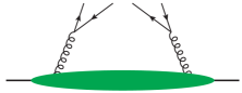
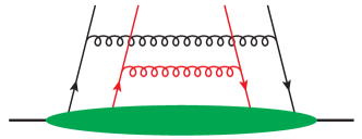
Figure 4: Left: graph for the splitting of one parton into two. Right: ladder graph for the independent scale evolution of the two partons.

Let us now discuss the scale dependence of double parton distributions. For the transverse-momentum dependent functions $F(x_{1},x_{2},\boldsymbol{k}_{1},\boldsymbol{k}_{2},\boldsymbol{y})$ one can derive Collins-Soper evolution equations in close analogy to the case of TMDs, as shown in Ref. [Diehl:2011yj]. Their solution naturally provides the Sudakov factors that resum large logarithms of $\boldsymbol{q}_{i}^{2}/Q^{2}$ in the TMD factorization formula. The evolution of collinear double parton distributions with color correlations has been discussed in Ref. [Manohar:2012jr] and is again closely related with the Sudakov logarithms we already mentioned in the previous section.

Collinear double parton distributions without color correlations follow DGLAP-type evolution equations. Two different versions of these have been discussed in the literature. It is natural to define the $\boldsymbol{y}$ space distributions for unpolarized partons as

$$F(x_{1},x_{2},\boldsymbol{y};\mu)$$

$$\quad=2p^{+}\!\!\int dy^{-}\,\frac{dz_{1}^{-}dz_{2}^{-}}{(2\pi)^{2}}\;e^{ip^{+}(x_{1}z_{1}^{-}+x_{2}z_{2}^{-})}\,\bigl{\langle}p\big{|}\mskip 1.5mu\mathcal{O}(y,z_{1};\mu)\,\mathcal{O}(0,z_{2};\mu)\mskip 1.5mu\big{|}p\bigr{\rangle}\,,$$ (7)

where

$$\mathcal{O}(y,z;\mu) =\tfrac{1}{2}\mskip 1.5mu\bigl{[}\bar{q}\bigl{(}-\tfrac{1}{2}z+y\bigr{)}\mskip 1.5mu\gamma^{+}q\bigl{(}\tfrac{1}{2}z+y\bigr{)}\bigr{]}_{\mu}\,, z^{+}=y^{+}=0\,,\boldsymbol{z}=\boldsymbol{0}$$ (8)

are the familiar twist-two light-cone operators, renormalized at scale $\mu$ in the same way as for single parton distributions. We note in passing that $F(x_{1},x_{2},\boldsymbol{y};\mu)$ involves the product of two twist-two operators at a spacelike distance $y$ from each other, which is to be distinguished from a twist-four operator. The scale dependence then follows a homogeneous DGLAP equation

$$\frac{d}{d\log\mu^{2}}\,F(x_{1},x_{2},\boldsymbol{y};\mu) =P\otimes_{x_{1}}F+P\otimes_{x_{2}}F\,,$$ (9)

where $P$ is the well-known DGLAP splitting kernel and $\otimes_{x_{i}}$ the corresponding convolution product for the variable $x_{i}$. A sum over the relevant parton species on the r.h.s. is understood. Eq. (9) describes the independent evolution of the two partons, as sketched in the right panel of Fig. 4. A study of the scale dependence of two-parton correlations in this framework can be found Ref. [Diehl:2014vaa] and in the presentation [TomasEvolution] at this workshop.

If one integrates $F(x_{1},x_{2},\boldsymbol{y};\mu)$ over $\boldsymbol{y}$, for instance in the Fourier transform from $\boldsymbol{y}$ to $\boldsymbol{r}$, the short-distance behavior (6) generates a further singularity in the form of a divergent integral $\int d\boldsymbol{y}^{2}/\boldsymbol{y}^{2}$. An appropriate ultraviolet subtraction then leads to the inhomogeneous evolution equation

$$\frac{d}{d\log\mu^{2}}\,F(x_{1},x_{2},\boldsymbol{r};\mu) =P\otimes_{x_{1}}F+P\otimes_{x_{2}}F+\frac{f(x_{1}+x_{2})}{x_{1}+x_{2}}\,K\Bigl{(}\frac{x_{1}}{x_{1}+x_{2}}\Bigr{)}\,,$$ (10)

which has been studied extensively in the literature.[15, 16, 17, 18] This equation has the attractive feature that it conserves sum rules for parton number and momentum if those are satisfied for $\boldsymbol{r}=\boldsymbol{0}$ at some starting scale.[17]

Which of the two evolution equations is relevant for the description of double scattering processes can only be answered if one specifies the factorization formula in which the distributions appear. The homogeneous version (9) leads to a scale dependence of the distributions that cancels the scale dependence of the hard-scattering cross sections $\hat{\sigma}_{1}$ and $\hat{\sigma}_{2}$ in the generalization of (1) to higher orders, whereas simply plugging distributions following the inhomogeneous evolution (10) into the same formula leaves an unphysical $\mu$ dependence in the $pp$ cross section.

In fact, the short-distance behavior (6) leads to a much more severe problem: when inserted into the factorization formula (1) it gives an integral diverging like $\int d\boldsymbol{y}^{2}/\boldsymbol{y}^{4}$. This ultraviolet divergence is connected with a further problem, noticed already in Ref. [Cacciari:2009dp] and later exhibited in Refs. [Diehl:2011tt,Diehl:2011yj]. The left panel in Fig. 5 represents double hard scattering with a perturbative splitting (cf. Fig. 4) in both protons, but at the same time it can be regarded as a two-loop contribution to diboson production by gluon-gluon fusion. Neither in the two-loop expression for single hard scattering nor in the double scattering formula (1) is there anything that prevents double counting of this graph in the region where the quark and antiquark coupling to a gluon are near collinear. A consistent description therefore requires an appropriate modification of one or both expressions. There is at present no consensus on how to deal with this problem; different points of view are discussed in Refs. [Diehl:2011yj,Gaunt:2011xd,Blok:2011bu,Ryskin:2011kk,Ryskin:2012qx].

         

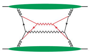
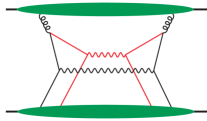
Figure 5: Graphs for the production of two gauge bosons involving the splitting $g\to q\bar{q}$ in one or both protons.

A further issue in this context is the treatment of the right panel in Fig. 5, where we have a short-distance $g\to q\bar{q}$ splitting in only one of the colliding protons. This graph and its phenomenological relevance has been discussed in Refs. [Blok:2011bu,Ryskin:2011kk,Ryskin:2012qx,Blok:2013bpa,Gaunt:2012dd].

Perhaps surprisingly, a consistent theory of double parton scattering thus even requires us to define what exactly we mean by “double parton scattering”, with some amount of freedom to shift contributions between single and double scattering terms.

References

- [1] N. Paver and D. Treleani, Nuovo Cim. A70, 215 (1982).
- [2] M. Mekhfi, Phys. Rev. D32, 2371 (1985).
- [3] M. Diehl and A. Schäfer, Phys. Lett. B698, 389 (2011) [arXiv:1102.3081].
- [4] M. Diehl, D. Ostermeier and A. Schäfer, JHEP 1203, 089 (2012) [arXiv:1111.0910].
- [5] M. Braun and D. Treleani, Eur. Phys. J. C 18, 511 (2001) [hep-ph/0005078].
- [6] M. Burkardt, Phys. Rev. D 62, 071503 (2000) [Erratum-ibid. D 66, 119903 (2002)] [hep-ph/0005108].
- [7] B. Blok, Yu. Dokshitzer, L. Frankfurt and M. Strikman, Phys. Rev. D 83, 071501 (2011) [arXiv:1009.2714].
- [8] M. Diehl, PoS DIS 2013, 074 (2013) [arXiv:1306.6480].
-
[9]
L. Frankfurt, M. Strikman and C. Weiss,
Phys. Rev. D 69, 114010 (2004)
[hep-ph/0311231]. - [10] T. Kasemets and M. Diehl, JHEP 1301, 121 (2013) [arXiv:1210.5434].
- [11] M. Mekhfi and X. Artru, Phys. Rev. D 37, 2618 (1988).
-
[12]
A. V. Manohar and W. J. Waalewijn,
Phys. Rev. D 85, 114009 (2012)
[arXiv:1202.3794]. - [13] M. Diehl, T. Kasemets and S. Keane, JHEP 1405, 118 (2014) [arXiv:1401.1233].
- [14] T. Kasemets, these proceedings.
- [15] R. Kirschner, Phys. Lett. B 84, 266 (1979).
- [16] V. P. Shelest, A. M. Snigirev and G. M. Zinovev, Phys. Lett. B 113, 325 (1982).
- [17] J. R. Gaunt and W. J. Stirling, JHEP 1003, 005 (2010) [arXiv:0910.4347].
- [18] F. A. Ceccopieri, arXiv:1403.2167.
- [19] M. Cacciari, G. P. Salam and S. Sapeta, JHEP 1004, 065 (2010) [arXiv:0912.4926].
- [20] J. R. Gaunt and W. J. Stirling, JHEP 1106, 048 (2011) [arXiv:1103.1888].
- [21] B. Blok, Yu. Dokshitzer, L. Frankfurt and M. Strikman, Eur. Phys. J. C 72, 1963 (2012) [arXiv:1106.5533].
- [22] M. G. Ryskin and A. M. Snigirev, Phys. Rev. D 83, 114047 (2011) [arXiv:1103.3495].
- [23] M. G. Ryskin and A. M. Snigirev, Phys. Rev. D 86, 014018 (2012) [arXiv:1203.2330].
- [24] B. Blok, Yu. Dokshitzer, L. Frankfurt and M. Strikman, Eur. Phys. J. C 74, 2926 (2014) [arXiv:1306.3763].
- [25] J. R. Gaunt, JHEP 1301, 042 (2013) [arXiv:1207.0480].