Model Selection and Estimation with Quantal-Response Data in Benchmark Risk Assessment

Abstract

This paper describes several approaches for estimating the benchmark dose (BMD) in a risk assessment study with quantal dose-response data and when there are competing model classes for the dose-response function. Strategies involving a two-step approach, a model-averaging approach, a focused-inference approach, and a nonparametric approach based on a PAVA-based estimator of the dose-response function are described and compared. Attention is raised to the perils involved in data “double-dipping” and the need to adjust for the model-selection stage in the estimation procedure. Simulation results are presented comparing the performance of five model selectors and eight BMD estimators. An illustration using a real quantal-response data set from a carcinogenecity study is provided.

Key Words and Phrases: Focused-inference approach; Information measures; Model selection problem; Model averaging; Pooled adjacent violators algorithm (PAVA); Quantal-dose response; Two-step estimation approach.

1 Introduction and Motivation

The traditional approach to statistical inference assumes that a random entity $\mathbf{Y}$, taking values in a sample space $\mathcal{Y}$, is observable. Such a $\mathbf{Y}$ represents the outcome of an experiment, a study, or a survey. The (joint) distribution function $F$ of $\mathbf{Y}$ is assumed to belong to a specified model class $\mathcal{F}$ of distribution functions on $\mathcal{Y}$. The class $\mathcal{F}$ may be parametrically or nonparametrically specified. For example, in quantal-response risk assessment studies of exposures to hazardous agents, the primary focus of this paper, there will be pre-specified doses $0=d_{1}<d_{2}<\ldots<d_{J}<\infty$, and for each dose $d_{j}$, there is an observable random variable $Y_{j}$, which is binomially distributed with parameters $N_{j}$ and $\pi(d_{j})$. Here, $N_{j}$ represents the number of units placed on test at dose $d_{j}$, $\pi(\cdot)$ is the dose-response function, $\pi(d_{j})$ is the probability of a unit at dose $d_{j}$ exhibiting the adverse event of interest, and $Y_{j}$ is the total out of the $N_{j}$ units that exhibit the adverse event [23, Ch. 4]. Commonly, we assume that the $N_{j}$s are known, the $Y_{j}$s are independent, and $\pi(\cdot)$ belongs to some model class $\mathcal{M}$. An example of a model class in this setting is

$$\mathcal{M}_{1}=\{\pi_{1}(d;\theta_{0},\theta_{1})=1-\exp\{-\theta_{0}-\theta_{1}d\}:\theta_{0}\in\Re_{+},\theta_{1}\in\Re_{+}\}.$$

This is the linear complementary log model, also known as the quantal-linear model or the one-stage model in carcinogenesis testing [3]. Typically, statistical attention will focus on making inferences about the unknown parameters, e.g., constructing a $100(1-\alpha)\%$ confidence interval on $\theta_{1}$. In risk assessment studies, however, the function $\pi(d_{j})$ is specifically used to model the risk of exhibiting an adverse response or reaction at dose $d_{j}$. Attention is then directed at using information in $\pi(\cdot)$ to estimate risk at low doses. By inverting the estimated dose-response relationship, the analyst can calculate the dose level at which a predetermined benchmark response (BMR) for the adverse response is attained. The corresponding Benchmark Dose (BMD), is an important quantity in deriving regulatory limits for modern risk management [23, § 4.3]. BMDs are employed increasingly in quantitative risk analyses for setting acceptable levels of human exposure or to establish modern low-exposure guidelines for hazardous environmental or chemical agents [29].

If $\mathbf{Y}\equiv(Y_{j},j=1,2,\ldots,J)$ is the observable vector from such a study, then its joint probability mass function $p_{\mathbf{Y}}$, which determines $F$, is

$$p_{\mathbf{Y}}(y_{1},\ldots,y_{J};\theta_{0},\theta_{1})=\prod_{j=1}^{J}\left(\begin{array}[]{c}N_{j}\\ y_{j}\end{array}\right)\pi_{1}(d_{j};\theta_{0},\theta_{1})^{y_{j}}[1-\pi_{1}(d_{j};\theta_{0},\theta_{1})]^{N_{j}-y_{j}}$$

for $y_{j}\in\{0,1,2,\ldots,N_{j}\}$. In this conventional framework with one model class, methods of inference, e.g., estimation, hypothesis testing, interval estimation, or prediction, are well-developed, relying on the maximum likelihood (ML) principle, the Neyman-Pearson hypothesis testing framework, or the Bayesian paradigm [8, 19, 17, 37].

Recent years, however, have seen greater appreciation for settings with more than one model class for $F$ [4, 7]. Such situations arise in a variety of scientific settings, including engineering, reliability, economics, and in particular, in the risk assessment problem emphasized herein [2, 28]. An impetus for considering several model classes is the desire for more inferential robustness without becoming fully nonparametric. For example, in the quantal-response setting, the dose-response function $\pi(\cdot)$, aside from being possibly in the model class $\mathcal{M}_{1}$, may alternatively belong to the model class

$$\mathcal{M}_{2}=\{\pi_{2}(d;\eta_{0},\eta_{1})={[1+\exp\{-(\eta_{0}+\eta_{1}d)\}]}^{-1}:\eta_{0}\in\Re,\eta_{1}\in\Re\},$$

In settings with multiple model classes, a seemingly natural approach is to use the data to first select the model class, and then use the same data again to perform inference in the chosen model class. However, caution needs to be exercised since, when not properly adjusting for such data “double-dipping,” detrimental consequences, such as underestimation of standard errors, loss of control of Type I error probabilities, or nonfulfillment of coverage probabilities, ensue [7, § 7.4]. It is of importance to examine issues pertaining to these statistical problems when operating with several possible model classes and to develop appropriate statistical procedures that properly adjust for data re-use. This paper is targeted for this purpose, with particular emphasis on quantal dose-response modeling and its use in estimating the benchmark dose for low-dose risk assessment.

2 Mathematical Underpinnings

We describe in this section the mathematical framework and formally state the problems of interest. Consider a quantal-response study where the collection $(\mathbf{N},\mathbf{d})=\{(N_{j},d_{j}),j=1,2,\ldots,J\}$ is given and the random observables are $\mathbf{Y}=(Y_{j},j=1,2,\ldots,J),$ where

$$Y_{j}|(N_{j},d_{j})\sim B(N_{j},\pi(d_{j})),j=1,2,\ldots,J.$$ (1)

Here $0=d_{1}<d_{2}<\ldots<d_{J}$ are the doses, $\pi(\cdot)$ is the dose-response function, and $B(n,\pi)$ is a binomial distribution with parameters $(n,\pi)$. The entire data ensemble will be denoted by $(\mathbf{Y},\mathbf{N},\mathbf{d})=\{(Y_{j},N_{j},d_{j}),j=1,2,\ldots,J\}$.

In most risk-analytic studies, the differential risk adjusted for any spontaneous or background effect is typically of interest. This leads to consideration of risks in excess of the background. Quantifying this, suppose the dose-response function is $\pi:\Re\rightarrow[0,1]$. Then, the extra risk function, which is relative to the background risk, is

$$\pi_{E}(d)=\frac{\pi(d)-\pi(0)}{1-\pi(0)}.$$ (2)

Typically it is assumed that the mapping $d\mapsto\pi(d)$ is monotone increasing, hence $d\mapsto\pi_{E}(d)$ is also monotone increasing. Given a BMR value $q\in(0,1)$, the BMD at this risk level $q$, denoted $\mbox{\emph{BMD}}(q)$, is the dose $d\geq 0$ satisfying $\pi_{E}(d)=q.$ For brevity, instead of writing $\mbox{\emph{BMD}}(q)$, we instead use the notation $\xi_{q}$, so

$$\xi_{q}\equiv BMD(q)=\pi_{E}^{-1}(q)$$ (3)

where $\pi_{E}^{-1}(\cdot)$ is the inverse function of $\pi_{E}(\cdot)$. Observe that $\xi_{q}$ is determined by the dose-response function and its parameters. In this paper we will mainly be concerned with obtaining estimators of $\xi_{q}$ and their properties.

We describe the mathematical set-up of interest. Our underlying assumption is that the unknown dose-response function $\pi(\cdot)$ is a member of the collection

$$\mathcal{M}=\mathcal{M}_{0}\cup\left(\cup_{m=1}^{M}\cup_{l=1}^{L_{m}}\mathcal{M}_{ml}\right),$$ (4)

where $\mathcal{M}_{0}$ and $\mathcal{M}_{ml},l=1,2,\ldots,L_{m};m=1,2,\ldots,M$, are model classes of dose-response functions. We assume that these model classes satisfy the following conditions:

• (C1) For each $m=1,2,\ldots,M$, we have $\mathcal{M}_{0}\subset\mathcal{M}_{m1}\subset\mathcal{M}_{m2}\subset\ldots\subset\mathcal{M}_{mL_{m}}.$

• (C2) The model classes are, for $m=1,2,\ldots,M$ and $l=1,2,\ldots,L_{m}$, of forms

  $$\mathcal{M}_{0}=\{\pi_{0}(\cdot;\theta_{0}):\theta_{0}\in\Theta_{0}\};$$

  $$\mathcal{M}_{ml}=\{\pi_{ml}(\cdot;\theta_{0},\theta_{m1},\ldots,\theta_{ml}):\theta_{0}\in\Theta_{0},\theta_{mj}\in\Theta_{mj},j=1,2,\ldots,l\},$$

  with $\Theta_{0}$ an open subset of $\Re^{g_{0}}$ and $\Theta_{mj}$ an open subset of $\Re^{g_{mj}}$, and with the dimensions $g_{0}$ and $g_{mj}$s being known.

• (C3) For each $m=1,2,\ldots,M$ and $l=1,2,\ldots,L_{m}$, there are unique elements $\{\theta_{ml}^{0}:l=1,2,\ldots,L_{m};m=1,2,\ldots,M\}$ such that $\theta_{ml}^{0}\in\Theta_{ml}$ and

  $$\pi_{ml-1}(\cdot;\theta_{0},\theta_{m1},\theta_{m2},\ldots,\theta_{ml-1})=\pi_{ml}(\cdot;\theta_{0},\theta_{m1},\theta_{m2},\ldots,\theta_{ml-1},\theta_{ml}^{0}).$$

• (C4) For each $m\neq m^{\prime}$, and for $l=1,2,\ldots,L_{m}$ and $l^{\prime}=1,2,\ldots,L_{m^{\prime}}$,

  $$\left(\mathcal{M}_{ml}\setminus\mathcal{M}_{0}\right)\cap\left(\mathcal{M}_{m^{\prime}l^{\prime}}\setminus\mathcal{M}_{0}\right)=\emptyset.$$

Conditions (C1-C3) imply that $\mathcal{M}_{0}$, which may be empty, is the smallest model class, and for each model type $m$, there is a nested structure among the layers $(\mathcal{M}_{ml},l=1,2,\ldots,L_{m})$. Condition (C4) requires that the $M$ model classes may only intersect at the smallest model class $\mathcal{M}_{0}$. Pictorially, the structure and inter-relationships among the model classes are shown in Figure 1. There are several commonly-used dose-response model classes. See, for instance, [2, 35, 36] for some examples.

With this mathematical framework in hand, our main objective is to obtain estimators of $\xi_{q}$ based on the observable $(\mathbf{Y},\mathbf{N},\mathbf{d})$. Apart from estimation of $\xi_{q}$, it is also of interest to determine the smallest or most parsimonious model class containing the dose-response function $\pi(\cdot)$, the so-called model selection problem.

Figure 1: Depiction of the interrelationships among the model classes. The columns represent the model class type, while the rows are the depths within the model class type. Note that the maximal depths, $L_{m}$, within each $m$th model class type may differ.

Model Class Type Depth	Model Class Type
$l$	$m$
0	$\mathcal{M}_{0}$
	$\cap$	$\cap$		$\cap$
1	$\mathcal{M}_{11}$	$\mathcal{M}_{21}$	$\cdots$	$\mathcal{M}_{M1}$
	$\cap$	$\cap$		$\cap$
2	$\mathcal{M}_{12}$	$\mathcal{M}_{22}$	$\cdots$	$\mathcal{M}_{M2}$
	$\cap$	$\cap$		$\cap$
$\vdots$	$\vdots$	$\vdots$	$\vdots$	$\vdots$
	$\cap$	$\cap$		$\cap$
$L_{m}$	$\mathcal{M}_{1L_{1}}$	$\mathcal{M}_{2L_{2}}$	$\cdots$	$\mathcal{M}_{ML_{M}}$

3 Model Class Selection

There are several approaches to the model selection problem. Most apply some form of information-theoretic metric to distinguish among competing models/model classes. Two popular measures are Akaike’s information criterion (AIC) [1] and the Bayesian information criterion (BIC) [30]. Both criteria are likelihood-based. Other forms are possible, including a second-order adjusted AIC [13], the Focused IC [7, § 6.2], Takeuchi’s IC [32], the Kullback-Leibler IC [5]. The AIC and BIC remain the most popular forms used in risk-analytic settings [28, 2, 10].

Given the quantal-response data $(\mathbf{y},\mathbf{N},\mathbf{d})$ and a model $\mathcal{M}$ which specifies a dose-response function $\pi(\cdot;\theta)$ with $\theta\in\Theta$, the likelihood function is

$$L(\theta|\mathcal{M})=L(\theta|\mathcal{M};(\mathbf{y},\mathbf{N},\mathbf{d}))=\prod_{j=1}^{J}\left(\begin{array}[]{c}N_{j}\\ y_{j}\end{array}\right)\pi(d_{j};\theta)^{y_{j}}[1-\pi(d_{j};\theta)]^{N_{j}-y_{j}},$$ (5)

so the relevant portion of the log-likelihood function $\log L(\theta|\mathcal{M})$ is

$$l(\theta|\mathcal{M})=\sum_{j=1}^{J}\left\{y_{j}\log\pi(d_{j};\theta)+(N_{j}-y_{j})\log[1-\pi(d_{j};\theta)]\right\}.$$ (6)

The maximum likelihood estimate (MLE) of $\theta$ under $\mathcal{M}$ is

$$\hat{\theta}=\hat{\theta}(\mathbf{y},\mathbf{N},\mathbf{d})=\arg\max_{\theta\in\Theta}L(\theta|\mathcal{M};(\mathbf{y},\mathbf{N},\mathbf{d}))=\arg\max_{\theta\in\Theta}l(\theta|\mathcal{M}).$$ (7)

The AIC for model $\mathcal{M}$ is

$$AIC(\mathcal{M})=-2l(\hat{\theta}|\mathcal{M})+2g$$ (8)

where $g$ is the dimension of $\Theta$, The BIC is

$$BIC(\mathcal{M})=-2l(\hat{\theta}|\mathcal{M})+g\log(n)$$ (9)

where $n=\sum_{j=1}^{K}N_{j}$ is the total number of units.

In the presence of several competing models $\{\mathcal{M}_{m}:m=1,2,\ldots,M\}$, the index of the chosen model class using the AIC or BIC approaches are, respectively,

$$\hat{M}_{AIC}(\mathbf{y},\mathbf{N},\mathbf{d}) = \arg\min_{m=1,2,\ldots,M}AIC(\mathcal{M}_{m}|\mathbf{y},\mathbf{N},\mathbf{d});$$ (10)

$$\hat{M}_{BIC}(\mathbf{y},\mathbf{N},\mathbf{d}) = \arg\min_{m=1,2,\ldots,M}BIC(\mathcal{M}_{m}|\mathbf{y},\mathbf{N},\mathbf{d}).$$ (11)

We employ these two model selection approaches to the quantal-response problem. To simplify our notation, let $\mathcal{M}_{m0}\equiv\mathcal{M}_{0}$ and $\Theta_{m0}\equiv\Theta_{0}$. Recall that

$$g_{ml}=\dim{\Theta}_{ml},\ l=0,1,2,\ldots,L_{m};m=1,2,\ldots,M,$$

the dimension of the sub-parameter space $\Theta_{ml}$ of $\mathcal{M}_{ml}$. The AIC and BIC become, for $l=0,1,2,\ldots,L_{m};m=1,2,\ldots,M$,

$$AIC(\mathcal{M}_{ml}) = -2l(\hat{\theta}_{0},\hat{\theta}_{m1},\ldots,\hat{\theta}_{ml}|\mathcal{M}_{ml})+2\left(g_{0}+\sum_{i=1}^{l}g_{mi}\right);$$ (12)

$$BIC(\mathcal{M}_{ml}) = -2l(\hat{\theta}_{0},\hat{\theta}_{m1},\ldots,\hat{\theta}_{ml}|\mathcal{M}_{ml})+\left(g_{0}+\sum_{i=1}^{l}g_{mi}\right)\log(n),$$ (13)

where $(\hat{\theta}_{0},\hat{\theta}_{m1},\ldots,\hat{\theta}_{ml})$ is the MLE of $(\theta_{0},\theta_{m1},\ldots,\theta_{ml})$ under model $\mathcal{M}_{ml}$. Observe that $(\hat{\theta}_{0},\hat{\theta}_{m1},\ldots,\hat{\theta}_{ml-1}),$ the MLE under model class $\mathcal{M}_{ml-1}$ coincides with the restricted MLE of $(\theta_{0},\theta_{m1},\ldots,\theta_{ml-1})$ under model class $\mathcal{M}_{ml}$ under the restriction $\theta_{ml}=\theta_{ml}^{0}$.

Model class $\mathcal{M}_{m^{*}l^{*}}$ will then be chosen according to the AIC approach whenever

$$AIC(\mathcal{M}_{m^{*}l^{*}})=\min_{m=1,2,\ldots,M}\min_{l=0,1,2\ldots,L_{m}}AIC(\mathcal{M}_{ml});$$

while it will be chosen via the BIC approach whenever

$$BIC(\mathcal{M}_{m^{*}l^{*}})=\min_{m=1,2,\ldots,M}\min_{l=0,1,2\ldots,L_{m}}BIC(\mathcal{M}_{ml}).$$

We point out that, though of interest by itself, the model class selection problem is not the primary aim in these risk benchmarking studies. Rather, of more importance is estimation of the BMD $\xi_{q}$. Thus, the model class selection aspect, though possibly crucial in the inferential process, acquires a somewhat secondary role. In the next two sections, we describe approaches for estimating $\xi_{q}$ which take into account the model class selection step.

4 Two-Step BMD Estimation Approach

Let us suppose that the true underlying model class is $\mathcal{M}_{ml}$ for some $l\in\{0,1,2,\ldots,L_{m}\}$ and $m\in\{1,2,\ldots,M\}$, with true dose-response function $\pi_{ml}(\cdot;\theta_{0},\theta_{m1},\ldots,\theta_{ml}).$ Denote its associated extra risk function by

$$\pi_{ml,E}(d;\theta_{0},\theta_{m1},\ldots,\theta_{ml})=\frac{\pi_{ml}(d;\theta_{0},\theta_{m1},\ldots,\theta_{ml})-\pi_{ml}(0;\theta_{0},\theta_{m1},\ldots,\theta_{ml})}{1-\pi_{ml}(0;\theta_{0},\theta_{m1},\ldots,\theta_{ml})},$$

and the inverse of this extra risk function by $\pi_{ml,E}^{-1}(\cdot;\theta_{0},\theta_{m1},\ldots,\theta_{ml})$. Then, under model class $\mathcal{M}_{ml}$, the BMD for a fixed $q=\mbox{BMR}$ is

$$\xi_{q|ml}(\theta_{0},\theta_{m1},\ldots,\theta_{ml})=\pi_{ml,E}^{-1}(q;\theta_{0},\theta_{m1},\ldots,\theta_{ml}).$$ (14)

It is natural to apply the substitution estimator where $(\theta_{0},\theta_{m1},\ldots,\theta_{ml})$ in (14) is replaced by its ML estimate under model class $\mathcal{M}_{ml}$. Thus, if $(\hat{\theta}_{0},\hat{\theta}_{m1},\ldots,\hat{\theta}_{ml})$ is the ML estimator under model class $\mathcal{M}_{ml}$ based on $(\mathbf{Y},\mathbf{N},\mathbf{d})$, then the estimator of $\xi_{q|ml}$ is

$$\hat{\xi}_{q|ml}=\xi_{q|ml}(\hat{\theta}_{0},\hat{\theta}_{m1},\ldots,\hat{\theta}_{ml})=\pi_{ml,E}^{-1}(q;\hat{\theta}_{0},\hat{\theta}_{m1},\ldots,\hat{\theta}_{ml}).$$ (15)

One approach to estimating the BMD among several competing model classes is to combine the model selection and estimation steps into a two-step approach [14, 10, 28]. The idea is to use the data to select the model class, either via AIC or BIC, and having chosen the model class, obtain the estimate of the BMD in the chosen model class, but with the estimate still based on the same data utilized in the model class selection step.

Under our framework let us then suppose that we have decided on a model class selection procedure, either AIC or BIC. Denote by

$$(\hat{m},\hat{l})\equiv\left(\hat{m}(\mathbf{Y},\mathbf{N},\mathbf{d}),\hat{l}(\mathbf{Y},\mathbf{N},\mathbf{d})\right)$$ (16)

the resulting model type index and the model type depth, respectively, of the selected model class. The two-step estimator of the BMD is then given by

$$\hat{\xi}_{q}^{TS}\equiv\hat{\xi}_{q}^{TS}(\mathbf{Y},\mathbf{N},\mathbf{d}))={\xi}_{q|\hat{m}(\mathbf{Y},\mathbf{N},\mathbf{d}))\,\hat{l}(\mathbf{Y},\mathbf{N},\mathbf{d})}(\mathbf{Y},\mathbf{N},\mathbf{d}).$$ (17)

In (17) we have explicitly shown where the data enter the picture. The difficulty in these two-step estimators is the re-use (“double-dipping”) of the data $(\mathbf{Y},\mathbf{N},\mathbf{d})$ since we use them to select the model class indices $(\hat{m},\hat{l})$, and then we again use them to estimate the BMD within the chosen model class. In assessing the properties of such two-step estimators, it is imperative that the impact of this data double-dipping be taken into account. Unless corrected for this additional stochastic element of the estimation process, confidence regions and significance tests will not possess the desired coverage levels or correct error rates; see, for instance, [6, 9].

5 Model-Averaging Approach to BMD Estimation

Another approach to estimating $\xi_{q}$ is via a model-averaging procedure; see, for instance, [12, 4, 11, 9]. The idea here is to combine estimates from the different model classes via some form of weighted average, with the weights constructed to quantify each model’s relative likelihood in describing the data. For our framework, we will specify data-dependent weights

$$\hat{\mathbf{w}}\equiv\hat{\mathbf{w}}(\mathbf{Y},\mathbf{N},\mathbf{d})=\{\hat{w}_{0},(\hat{w}_{ml},l=1,2,\ldots,L_{m},m=1,2,\ldots,M)\},$$

so that the associated model-averaged estimator of $\xi_{q}$ will be

$$\hat{\xi}_{q}^{MA}(\mathbf{Y},\mathbf{N},\mathbf{d})=\hat{w}_{0}(\mathbf{Y},\mathbf{N},\mathbf{d})\hat{\xi}_{q|0}(\mathbf{Y},\mathbf{N},\mathbf{d})+$$

$$\sum_{m=1}^{M}\sum_{l=1}^{L_{m}}\hat{w}_{ml}(\mathbf{Y},\mathbf{N},\mathbf{d})\hat{\xi}_{q|ml}(\mathbf{Y},\mathbf{N},\mathbf{d}).$$ (18)

There are several ways to specify the weights. Perhaps the simplest avenue is to impose a Bayesian structure to the problem, so that the weights become related to the posterior probabilities of each of the model classes [2, 18]. Here we describe the more conventional approach where the weights arise from the AIC or BIC values. The AIC-based weights are, for $m=1,2,\ldots,M$ and $l=0,1,2,\ldots,L_{m}$, computed according to the so-called Akaike weights [4, § 2.9] given by

$$\hat{w}_{ml}^{AIC}=\frac{\exp\{-\frac{1}{2}AIC(\mathcal{M}_{ml})\}}{\exp\{-\frac{1}{2}AIC(\mathcal{M}_{0})\}+\sum_{m=1}^{M}\sum_{l=1}^{L_{m}}\exp\{-\frac{1}{2}AIC(\mathcal{M}_{ml}\}}.$$ (19)

Observe that these weights are data-dependent since the AIC-values are derived from (12). Similarly, the data-dependent BIC weights are specified via

$$\hat{w}_{ml}^{BIC}=\frac{\exp\{-\frac{1}{2}BIC(\mathcal{M}_{ml})\}}{\exp\{-\frac{1}{2}BIC(\mathcal{M}_{0})\}+\sum_{m=1}^{M}\sum_{l=1}^{L_{m}}\exp\{-\frac{1}{2}BIC(\mathcal{M}_{ml}\}},$$ (20)

where the BIC values are computed using (13). In the above formulas, recall our earlier notation where a subscript of “_m0” coincides with the subscript ‘₀’ so that $\hat{w}_{m0}$ is $\hat{w}_{0}$.

As in the two-step estimator of $\xi_{q}$, investigating the theoretical properties of these model-averaged estimators is non-trivial owing to the dependence of both the model-averaging weights and the estimator of $\xi_{q}$ in each model class; see, for instance, the evaluation of the properties of such estimators in specific models in [9]. For this quantal-response problem, we will investigate the properties of these model-averaged estimators via computer simulation studies in a later section.

6 A Focused-Inference Approach

This section presents an approach which integrates the model selection and estimation steps. In contrast to the model class selection procedures in Section 3 which choose the model class without direct regard to the parameter of main interest, the focused-inference approach takes into consideration in the model class selection stage the fact that the BMD $\xi_{q}$ is the parameter of primary interest. This strategy was developed in [6, 11, 7]. Since the problem is of a general nature, we will first present the solution for the larger problem and then apply it to benchmark dose estimation.

6.1 Description of the General Setting

We suppose that for a sample size $n$ we are able to observe the realization of a random observable $X_{n}$ taking values in a sample space $\mathcal{X}_{n}$. We denote by $F_{n}$ the distribution function of $X_{n}$, and assume that $F_{n}\in\mathcal{F}\equiv\cup_{m=1}^{M}\mathcal{F}_{mn},$ where $\mathcal{F}_{mn}=\{F_{mn}(\cdot;\theta_{m}):\ \theta_{m}\in\Theta_{m}\}$ with $\Theta_{m}$ an open subset of $\Re^{g_{m}}$ for a known positive integer $g_{m}$. We denote by $f_{mn}(\cdot;\theta_{m})$ the density function of $F_{mn}(\cdot;\theta_{m})$ with respect to some dominating measure $\nu_{n}$, e.g., Lebesgue or counting measure. Model class $m\in\{1,2,\ldots,M\}$ will be $\mathcal{M}_{m}=\{\mathcal{F}_{mn}:\ n=1,2,\ldots\}.$

We suppose that the parameter of primary interest is a functional $\tau$ on $\mathcal{F}$ which takes the form

$$\tau=\sum_{m=1}^{M}\tau_{m}(\theta_{m})I\{F_{n}\in\mathcal{F}_{mn}\},$$ (21)

where $\tau_{m}:\Theta_{m}\rightarrow\Re$. We assume that each $\tau_{m}$ possesses ‘smoothness properties’ such as differentiability and continuity with respect to each $\theta_{m}$ component. In this general setting, the primary goal is to estimate $\tau$ based on $X_{n}$ and to obtain properties of the estimator. Of secondary interest is to determine a parsimonious model class containing $F_{n}$. We start by examining asymptotic properties of estimators of $\tau_{m}$ under the true model class and also under a misspecified model class.

6.2 Properties under True Model Class

First, let us consider the situation where model class $\mathcal{M}_{m}$ holds, so $F_{n}=F_{mn}(\cdot;\theta_{m})\equiv F_{mn}(\theta_{m})$ for some $\theta_{m}\in\Theta_{m}$. Thus, in the sequel, probability statements, including expectations, variances, and covariances, are taken with respect to $F_{mn}(\cdot;\theta_{m})$. Furthermore, we define the operators $\nabla\equiv\nabla_{\theta}=\frac{\partial}{\partial\theta}$ and $\nabla^{\otimes 2}\equiv\nabla_{\theta\theta^{\tt t}}=\frac{\partial^{2}}{\partial\theta\partial\theta^{\tt t}}.$ We let

$$\mathfrak{I}_{mn}(\theta_{m}) = E\left\{\left(\nabla_{\theta_{m}}\log f_{mn}(X_{n};\theta_{m})\right)^{\otimes 2}|F_{mn}(\theta_{m})\right\}$$ (22)

$$= -E\left\{\nabla_{\theta_{m}\theta_{m}^{\tt t}}\log f_{mn}(X_{n};\theta_{m})|F_{mn}(\theta_{m})\right\}$$

be the Fisher information matrix for model class $\mathcal{M}_{m}$. Then, under suitable regularity conditions and results from ML estimation theory [16, § 6.3], the sequence of MLEs $\{\hat{\theta}_{mn},n=1,2,\ldots\}$ based on the sequence of data $\{X_{n},n=1,2,\ldots\}$, under model class $\mathcal{M}_{m}$, is consistent for $\theta_{m}$ and has the asymptotic distributional property

$$\mathfrak{L}\left\{\sqrt{n}(\hat{\theta}_{mn}-\theta_{m})|F_{mn}(\theta_{m})\right\}\stackrel{{\scriptstyle d}}{{\longrightarrow}}N(0,\mathfrak{I}_{m}^{-1}(\theta_{m})),$$ (23)

where $\mathfrak{L}(\cdot|F_{mn}(\theta_{m}))$ denotes the distributional law under $F_{n}=F_{mn}(\theta_{m})$, and where

$$\mathfrak{I}_{m}(\theta_{m})\equiv{\rm plim}_{n\rightarrow\infty}\frac{1}{n}\mathfrak{I}_{mn}(\theta_{m}),$$

with ‘plim’ meaning convergence in probability. By the Delta Method [16, § 1.8], with $\stackrel{{\scriptstyle\bullet}}{{\tau}}_{m}(\theta_{m})=\nabla_{\theta_{m}}\tau_{m}(\theta_{m}),$ the following propostion follows.

Proposition 1

As $n\rightarrow\infty$,

$$\mathfrak{L}\left\{\sqrt{n}\left(\tau_{m}(\hat{\theta}_{mn})-\tau_{m}(\theta_{m})\right)|F_{mn}(\theta_{m})\right\}\stackrel{{\scriptstyle d}}{{\longrightarrow}}N(0,\stackrel{{\scriptstyle\bullet}}{{\tau}}_{m}(\theta_{m})^{\tt t}\mathfrak{I}_{m}^{-1}(\theta_{m})\stackrel{{\scriptstyle\bullet}}{{\tau}}_{m}(\theta_{m})).$$

6.3 Properties under a Misspecified Model Class

Next, we examine the properties of $\hat{\theta}_{mn}$ when the true model class is $\mathcal{M}_{m^{\prime}}$. This will enable us to obtain the properties of $\tau_{m}(\hat{\theta}_{mn})$ under the model class $\mathcal{M}_{m^{\prime}}$. Define the Kullback-Leibler divergence between $f_{mn}(\cdot;\theta_{m})$ and $f_{m^{\prime}n}(\cdot;\theta_{m^{\prime}})$, under $F_{m^{\prime}n}(\theta_{m^{\prime}})$, according to

$$K_{m,m^{\prime}}^{(n)}(\theta_{m},\theta_{m^{\prime}})=\int\log\left\{\frac{f_{mn}(x_{n};\theta_{m})}{f_{m^{\prime}n}(x_{n};\theta_{m^{\prime}})}\right\}f_{m^{\prime}n}(x_{n};\theta_{m^{\prime}})\nu_{n}(dx_{n}).$$ (24)

We also assume that there is a function $K_{m,m^{\prime}}:\Theta_{m}\times\Theta_{m^{\prime}}\rightarrow\Re$ such that

$$K_{m,m^{\prime}}(\theta_{m},\theta_{m^{\prime}})=\lim_{n\rightarrow\infty}\frac{1}{n}K_{m,m^{\prime}}^{(n)}(\theta_{m},\theta_{m^{\prime}}).$$ (25)

Define

$$\theta_{m,m^{\prime}}^{*(n)}(\theta_{m^{\prime}})=\arg\max_{\theta_{m}\in\Theta_{m}}K_{m,m^{\prime}}^{(n)}(\theta_{m},\theta_{m^{\prime}}),$$ (26)

so $f_{mn}(\cdot;\theta_{m,m^{\prime}}^{*(n)}(\theta_{m^{\prime}}))$ is the closest element of $\mathcal{F}_{mn}$ to the true density $f_{m^{\prime}n}(\cdot;\theta_{m^{\prime}})$ according to Kullback-Leibler divergence, also referred to as the quasi true model in the assumed model class $\mathcal{F}_{mn}$. We assume that

$$\lim_{n\rightarrow\infty}\theta_{m,m^{\prime}}^{*(n)}(\theta_{m^{\prime}})=\theta_{m,m^{\prime}}^{*}(\theta_{m^{\prime}})$$

where

$$\theta_{m,m^{\prime}}^{*}(\theta_{m^{\prime}})=\arg\max_{\theta_{m}\in\Theta_{m}}K_{m,m^{\prime}}(\theta_{m},\theta_{m^{\prime}}).$$ (27)

By Jensen’s Inequality [16, § 1.7] note that we have $K_{m,m^{\prime}}^{(n)}(\theta_{m},\theta_{m^{\prime}})\leq 0$ with equality iff $m=m^{\prime}$. In particular, $K_{m,m^{\prime}}^{(n)}(\theta_{m,m^{\prime}}^{*(n)}(\theta_{m^{\prime}}),\theta_{m^{\prime}})\leq 0$, with equality iff $m=m^{\prime}$, in which case $\theta_{m,m}^{*(n)}(\theta_{m})=\theta_{m}$. Furthermore, under suitable regularity conditions, note that $\theta_{m,m^{\prime}}^{*(n)}(\theta_{m^{\prime}})$ solves the equation

$$\int\left\{\nabla_{\theta_{m}}\log f_{mn}(x_{n};\theta_{m})\right\}f_{m^{\prime}n}(x_{n};\theta_{m^{\prime}})\nu_{n}(dx_{n})=0.$$ (28)

Let

$$U_{mn}(\theta_{m};x_{n})=\nabla_{\theta_{m}}\log f_{mn}(x_{n};\theta_{m})$$

be the score function of $\theta_{m}$, under $F_{mn}$, given data $x_{n}$. Then, from (28), we have that at $\theta_{m}=\theta_{mm^{\prime}}^{*(n)}(\theta_{m^{\prime}})$,

$$E\left\{U_{mn}(\theta_{m};X_{n})|F_{m^{\prime}n}(\theta_{m^{\prime}})\right\}=\int U_{mn}(\theta_{m};x_{n})f_{m^{\prime}n}(x_{n};\theta_{m^{\prime}})\nu_{n}(dx_{n})=0.$$

Let

$$A_{mn}(\theta_{m};x_{n})=-\nabla_{\theta_{m}\theta_{m}^{\tt t}}\log f_{mn}(x_{n};\theta_{m})$$

be the observed information matrix function under model $F_{mn}$ given data $x_{n}$. We assume that, under model class $\mathcal{M}_{m^{\prime}}$, there exists a vector function $U_{m,m^{\prime}}:\Theta_{m}\times\Theta_{m^{\prime}}\rightarrow\Re^{g}$ and a matrix function $A_{m,m^{\prime}}:\Theta_{m}\times\Theta_{m^{\prime}}\rightarrow(\Re^{g})^{\otimes 2}$ such that, under model class $\mathcal{M}_{m^{\prime}}$, we have

$$\frac{1}{n}U_{mn}(\theta_{m};X_{n})\stackrel{{\scriptstyle up}}{{\longrightarrow}}U_{m,m^{\prime}}(\theta_{m},\theta_{m^{\prime}})\quad\mbox{and}\quad\frac{1}{n}A_{mn}(\theta_{m};X_{n})\stackrel{{\scriptstyle up}}{{\longrightarrow}}A_{m,m^{\prime}}(\theta_{m},\theta_{m^{\prime}}),$$

where ‘$\stackrel{{\scriptstyle up}}{{\longrightarrow}}$’ means uniform convergence in probability. The required uniform convergence in probability is only needed in a neighborhood of $\theta_{mm^{\prime}}^{*}(\theta_{m^{\prime}})$. Note that $A_{m,m}(\theta_{m},\theta_{m})=\mathfrak{I}_{m}(\theta_{m}).$

We will now obtain the asymptotic distribution of the sequence of estimators $\{\hat{\theta}_{mn}(X_{n}):\ n=1,2,\ldots\}$ when the true model class is $\mathcal{M}_{m^{\prime}}$. By the defining property of $\hat{\theta}_{mn}$, we have $\frac{1}{n}U_{mn}(\hat{\theta}_{mn};X_{n})=0.$ Expanding this at $\theta_{m,m^{\prime}}^{*(n)}(\theta_{m^{\prime}})$, we achieve

$$0 = \frac{1}{\sqrt{n}}U_{mn}(\hat{\theta}_{mn};X_{n})$$

$$= \frac{1}{\sqrt{n}}U_{mn}\left(\theta_{m,m^{\prime}}^{*(n)}(\theta_{m^{\prime}});X_{n}\right)-\frac{1}{\sqrt{n}}A_{mn}(\tilde{\theta}_{n};X_{n})\left(\hat{\theta}_{mn}-\theta_{m,m^{\prime}}^{*(n)}(\theta_{m^{\prime}})\right),$$

where $\tilde{\theta}_{n}\in[\hat{\theta}_{mn},\theta_{m,m^{\prime}}^{*(n)}(\theta_{m^{\prime}})]$. Consequently,

$$\sqrt{n}\left(\hat{\theta}_{mn}-\theta_{m,m^{\prime}}^{*(n)}(\theta_{m^{\prime}})\right)=\left[\frac{1}{n}A_{mn}(\tilde{\theta}_{n};X_{n})\right]^{-1}\frac{1}{\sqrt{n}}U_{mn}\left(\theta_{m,m^{\prime}}^{*(n)}(\theta_{m^{\prime}});X_{n}\right).$$ (29)

Under suitable regularity conditions it can be shown that, under model class $\mathcal{M}_{m^{\prime}}$, $\hat{\theta}_{mn}\stackrel{{\scriptstyle p}}{{\longrightarrow}}\theta_{m,m^{\prime}}^{*}(\theta_{m^{\prime}})$. This implies that $\tilde{\theta}_{n}\stackrel{{\scriptstyle p}}{{\longrightarrow}}\theta_{m,m^{\prime}}^{*}(\theta_{m^{\prime}})$. As a consequence, we have that

$$\frac{1}{n}A_{mn}(\tilde{\theta}_{n};X_{n})\stackrel{{\scriptstyle p}}{{\longrightarrow}}A_{m,m^{\prime}}(\theta_{m,m^{\prime}}^{*}(\theta_{m^{\prime}}),\theta_{m^{\prime}}).$$

On the other hand, under model class $\mathcal{M}_{m^{\prime}}$, we assume that

$$\frac{1}{\sqrt{n}}U_{mn}\left(\theta_{m,m^{\prime}}^{*(n)}(\theta_{m^{\prime}}),X_{n}\right)\stackrel{{\scriptstyle d}}{{\longrightarrow}}N(0,\Sigma_{m,m^{\prime}}(\theta_{m,m^{\prime}}^{*}(\theta_{m^{\prime}}),\theta_{m^{\prime}})),$$ (30)

where, with $\Sigma_{m,m^{\prime}}^{(n)}(\theta_{m},\theta_{m^{\prime}})=Cov\left\{U_{mn}(X_{n};\theta_{m})|F_{m^{\prime}n}(\theta_{m^{\prime}})\right\},$ we have

$$\Sigma_{m,m^{\prime}}(\theta_{m,m^{\prime}}^{*}(\theta_{m^{\prime}}),\theta_{m^{\prime}}))=\lim_{n\rightarrow\infty}\frac{1}{n}\Sigma_{m,m^{\prime}}^{(n)}(\theta_{m,m^{\prime}}^{*(n)}(\theta_{m^{\prime}}),\theta_{m^{\prime}}).$$

Note that, for $m=1,2,\ldots,M$, we find $\Sigma_{m,m}(\theta_{m,m}^{*}(\theta_{m}),\theta_{m})=\mathfrak{I}_{m}(\theta_{m}).$ As a consequence, we have the following proposition:

Proposition 2

As $n\rightarrow\infty$,

$$\mathfrak{L}\left\{\sqrt{n}\left(\hat{\theta}_{mn}-\theta_{m,m^{\prime}}^{*(n)}(\theta_{m^{\prime}})\right)|\mathcal{M}_{m^{\prime}}\right\}\stackrel{{\scriptstyle d}}{{\longrightarrow}}N(0,\Xi_{m,m^{\prime}}(\theta_{m^{\prime}})),$$

where

$$\Xi_{m,m^{\prime}}(\theta_{m^{\prime}})=A_{m,m^{\prime}}^{-1}\left(\theta_{m,m^{\prime}}^{*}(\theta_{m^{\prime}}),\theta_{m^{\prime}}\right)$$

$$\Sigma_{m,m^{\prime}}(\theta_{m,m^{\prime}}^{*}(\theta_{m^{\prime}}),\theta_{m^{\prime}}))A_{m,m^{\prime}}^{-1}\left(\theta_{m,m^{\prime}}^{*}(\theta_{m^{\prime}}),\theta_{m^{\prime}}\right).$$

Finally, by applying the Delta Method, we obtain the following result concerning the asymptotic properties of ${\tau}(\hat{\theta}_{mn})$ under a misspecified model.

Theorem 1

As $n\rightarrow\infty$,

$$\mathfrak{L}\left\{\sqrt{n}\left(\tau_{m}(\hat{\theta}_{mn})-\tau_{m}(\theta_{m,m^{\prime}}^{*(n)}(\theta_{m^{\prime}}))\right)|\mathcal{M}_{m^{\prime}}\right\}\stackrel{{\scriptstyle d}}{{\longrightarrow}}N\left(0,\Gamma_{m,m^{\prime}}(\theta_{m^{\prime}})\right),$$

where $\Gamma_{m,m^{\prime}}(\theta_{m^{\prime}})=\ \stackrel{{\scriptstyle\bullet}}{{\tau}}_{m}(\theta_{m,m^{\prime}}^{*}(\theta_{m^{\prime}}))^{\tt t}\Xi_{m,m^{\prime}}(\theta_{m^{\prime}})\stackrel{{\scriptstyle\bullet}}{{\tau}}_{m}(\theta_{m,m^{\prime}}^{*}(\theta_{m^{\prime}})).$

We remark that the result in Proposition 1 can be recovered from Theorem 1 by noting that for each $m=1,\ldots,M$, we have $\theta_{m,m}^{*}(\theta_{m})=\theta_{m}$ and $\Gamma_{m,m}(\theta_{m})=\,\stackrel{{\scriptstyle\bullet}}{{\tau}}_{m}(\theta_{m})^{\tt t}\,\mathfrak{I}_{m}(\theta_{m})^{-1}\,\stackrel{{\scriptstyle\bullet}}{{\tau}}_{m}(\theta_{m}).$ In addition, we also point out that the true model need not actually be a parametric model. The derivations above, with a slight change in notation, also hold if the true model is simply represented by $\mathcal{M}^{\prime(n)}$ with the governing distribution of $F^{\prime(n)}(\cdot)$. In such a case, for the Kullback-Leibler divergence, we use the mapping

$$\theta_{m}\mapsto\int\log\{f_{mn}(x_{n};\theta_{m})\}F^{\prime(n)}(dx_{n}).$$

6.4 Rationale for the Focused-Inference Approach

Consider now a sequence of estimators for $\tau$, say $\{\hat{\tau}_{n}:\ n=1,2,3,\ldots\}$. How should we evaluate this sequence of estimators? Clearly, the evaluation will depend on the true value of $\tau$, which in turn depends on the model class that holds. A reasonable measure of the quality of this sequence of estimators would be

$$R_{m^{\prime}}(\hat{\tau}_{n},\theta_{m^{\prime}})=nE\left\{\left(\hat{\tau}_{n}-\tau_{m^{\prime}}(\theta_{m^{\prime}})\right)^{2}|\mathcal{M}_{m^{\prime}}\right\},n=1,2,3,\ldots.$$ (31)

This represents the (re-scaled) risk function, associated with squared-error loss, under model class $\mathcal{M}_{m^{\prime}}$. [Note that by ‘risk function’ here we mean expected loss, as in the usual decision-theoretic paradigm. This should not be confused with the extra risk function in (2) used to define the BMD.] To simplify our notation, let $\hat{\tau}_{mn}\equiv\tau_{m}(\hat{\theta}_{mn}),\ n=1,2,3,\ldots.$ Then, let $R_{m,m^{\prime}}^{(n)}(\theta_{m^{\prime}})\equiv R_{m^{\prime}}(\hat{\tau}_{mn},\theta_{m^{\prime}}).$ By using the identity

$$n\left(\tau_{m}(\hat{\theta}_{mn})-\tau_{m^{\prime}}(\theta_{m^{\prime}})\right)^{2}=$$

$$n\left[\left(\tau_{m}(\hat{\theta}_{mn})-\tau_{m}(\theta_{m,m^{\prime}}^{*}(\theta_{m^{\prime}}))\right)+\left(\tau_{m}(\theta_{m,m^{\prime}}^{*}(\theta_{m^{\prime}}))-\tau_{m^{\prime}}(\theta_{m^{\prime}})\right)\right]^{2},$$

we obtain from the earlier asymptotic results that, for large $n$,

$$R_{m,m^{\prime}}^{(n)}(\theta_{m^{\prime}})\approx\Gamma_{m,m^{\prime}}(\theta_{m^{\prime}})+n\left[\tau_{m}(\theta_{m,m^{\prime}}^{*}(\theta_{m^{\prime}}))-\tau_{m^{\prime}}(\theta_{m^{\prime}})\right]^{2},$$ (32)

a variance-bias decomposition. Note that to obtain (32), we also used the result that

$$E\{\sqrt{n}[\hat{\tau}_{n}-\tau_{m}(\theta_{m,m^{\prime}}^{*}(\theta_{m^{\prime}})]|\mathcal{M}_{m^{\prime}}\}=o(1).$$

Furthermore, observe that, for large $n$,

$$R_{m,m}^{(n)}(\theta_{m})\approx\Gamma_{m,m}(\theta_{m})=\,\stackrel{{\scriptstyle\bullet}}{{\tau}}_{m}(\theta_{m})^{\tt t}\,\mathfrak{I}_{m}(\theta_{m})^{-1}\,\stackrel{{\scriptstyle\bullet}}{{\tau}}_{m}(\theta_{m}).$$

We now describe possible approaches to utilizing the above risks for model selection and BMD estimation.

6.5 An Empirical-Based Approach

Presumably there is a sequence of true models $\{\mathcal{M}^{\prime}_{n}\}$ governing the data sequence $\{X_{n}\}$. We do not know this sequence of true models, and it need not coincide with the possible model classes under consideration, so we will not know the quantities $\theta_{\mathcal{M}^{\prime}}$ and $\theta^{*}_{m,\mathcal{M}^{\prime}}$. As such we will not know the risks $R_{m,{\mathcal{M}^{\prime}}}^{(n)}$.

A possible approach is to use a nonparametric estimate of $F_{n}^{\prime}$, say $\hat{F}_{n}^{\prime}$, and to use this estimate to obtain estimates of both $\tau_{\mathcal{M}^{\prime}}$ and $\theta_{m,\mathcal{M}^{\prime}}^{*}$. Let such estimates be $\hat{\tau}_{\mathcal{M}^{\prime}}^{(n)}$ and $\hat{\theta}_{m,\mathcal{M}^{\prime}}^{*(n)}$, the latter being the KL projection of $\hat{F}_{n}^{\prime}$ on $\Theta_{m}$. For each $m$ we may then estimate $R_{m,\mathcal{M}^{\prime}}$ by

$$\hat{R}_{m,\mathcal{M}^{\prime}}^{EMP,(n)}=\Gamma_{m,\mathcal{M}^{\prime}}(\hat{\theta}_{m,\mathcal{M}^{\prime}}^{*(n)})+n\left[\tau_{m}(\hat{\theta}_{m,\mathcal{M}^{\prime}}^{*(n)})-\hat{\tau}_{\mathcal{M}^{\prime}}^{(n)}\right]^{2}.$$

On the basis of these empirically estimated risks, a possible model selector is

$$\hat{m}^{EMP}=\arg\min_{m}\hat{R}_{m,\mathcal{M}^{\prime}}^{EMP},$$ (33)

and the associated BMD estimator is

$$\hat{\tau}_{n}^{EMP}=\tau_{\hat{m}^{EMP}}(\hat{\theta}_{\hat{m}^{EMP},n}).$$ (34)

6.6 A Model-Based Approach

Another approach to estimating the risks $R_{m,m^{\prime}}^{(n)}(\theta_{m^{\prime}})$ is by substituting for $\theta_{m^{\prime}}$ the estimator $\hat{\theta}_{m^{\prime}n}$. However, because we could not really be certain that model $\mathcal{M}^{\prime}$ is the true model, in estimating the bias term we replace $\tau_{\mathcal{M}^{\prime}}$ by an empirical estimator such as the one utilized in the preceding subsection. Observe that if we also estimate $\tau_{m^{\prime}}(\theta_{m^{\prime}})$ by $\tau_{m^{\prime}}(\hat{\theta}_{m^{\prime}})$, then the estimated bias term will always become zero whenever $m=m^{\prime}$. This would be fine if the actual underlying model truly belongs to the models under consideration, but this could be misleading if the true model class is not among the considered models. Hence, the rationale for the use of a nonparametric estimate of $\tau_{m^{\prime}}(\theta_{m^{\prime}})$ in estimating the bias term.

Now, denote the resulting estimator of $R_{m,m^{\prime}}(\theta_{m^{\prime}})$ by $\hat{R}_{m,m^{\prime}}^{(n)}$ for $n=1,2,3,\ldots$ and $m,m^{\prime}\in\{1,2,\ldots,M\}$. We may picture these risk estimates as in Table 1.

Table 1: Decision-theoretic risk estimates of different model class-based estimators under the possible model classes.

Estimator Based On	True Underlying Model Class
Model Class	$m^{\prime}$
$m$	$1$	$2$	$\cdots$	$M$
1	$\hat{R}_{1,1}^{(n)}$	$\hat{R}_{1,2}^{(n)}$	$\cdots$	$\hat{R}_{1,M}^{(n)}$
2	$\hat{R}_{2,1}^{(n)}$	$\hat{R}_{2,2}^{(n)}$	$\cdots$	$\hat{R}_{2,M}^{(n)}$
$\vdots$	$\vdots$	$\vdots$	$\vdots$	$\vdots$
$M$	$\hat{R}_{M,1}^{(n)}$	$\hat{R}_{M,2}^{(n)}$	$\cdots$	$\hat{R}_{M,M}^{(n)}$

Suppose for the moment that our goal is to select the model class that holds as informed by the parametric function $\tau$. For each possible model class $\mathcal{M}^{\prime}$, we may determine the estimator yielding the smallest risk. Having done so, we may then determine the model class that yields the smallest among these lowest risks. As such, a possible model class index selector, focused towards the estimation of $\tau$, is

$$\hat{m}^{FM}={\arg\min}_{m^{\prime}=1,2,\ldots,M}\left\{\min_{m=1,2,\ldots,M}\hat{R}_{m,m^{\prime}}^{(n)}\right\}.$$ (35)

This could be referred to as a $\tau$-focused model class selector. If the primary goal is to select the model class, then it will be $\mathcal{M}_{\hat{m}^{FM}}$. An associated BMD estimator will then be

$$\hat{\tau}^{FM}=\tau_{\hat{m}^{FM}}(\hat{\theta}_{\hat{m}^{FM}}).$$ (36)

As noted earlier, however, the model class selection problem is not of primary interest. Rather, we seek to estimate the parametric functional $\tau$. The viewpoint utilized in the development of the model class selector (35) may not therefore be the most appropriate in terms of choosing the estimator of $\tau$.

Instead, we argue as follows. Given the $\tau$-estimator based on model class $\mathcal{M}_{m}$, we may ask which model class $\mathcal{M}_{m^{\prime}}$ leads to the smallest risk. Having done so, we then ask which among the $M$ model class-based estimators yields the smallest among these lowest risks. This motivates the model class index selector

$$\hat{m}^{FE}={\arg\min}_{m=1,2,\ldots,M}\left\{\min_{m^{\prime}=1,2,\ldots,M}\hat{R}_{m,m^{\prime}}^{(n)}\right\}.$$ (37)

The resulting focused estimator of $\tau$ is

$$\hat{\tau}^{FE}=\tau_{\hat{m}^{FE}}(\hat{\theta}_{\hat{m}^{FE}}).$$ (38)

Note that $\hat{m}^{EMP}$, $\hat{m}^{FM}$, $\hat{m}^{FE}$, and $\hat{\theta}^{m}$ are all functions of the data $X_{n}$, hence the estimators of $\tau$ given by $\hat{\tau}^{EMP}$, $\hat{\tau}^{FM}$, and $\hat{\tau}^{FE}$ all possess a two-step flavor instead of a model-averaged flavor.

7 Application to Quantal-Response Problem

We now apply the theory presented in Section 6 to the quantal-response problem, where the random observable $X_{n}$ is $(\mathbf{Y},\mathbf{N},\mathbf{d})\equiv(\mathbf{Y}^{(n)},\mathbf{N}^{(n)},\mathbf{d}^{(n)})$ and the model classes are indexed by $(m,l)$, where $l\in\{0,1,2,\ldots,L_{m}\}$ and $m\in\{1,2,\ldots,M\}$. The parameter of interest that coincides with $\tau$ in the preceding section is the BMD $\xi_{q}$, defined by

$$\xi_{q}=\tau_{ml}(\theta_{0},\theta_{m1},\theta_{m2},\ldots,\theta_{ml};q)=\pi_{ml;E}^{-1}(q;\theta_{0},\theta_{m1},\theta_{m2},\ldots,\theta_{ml})$$

on model class $\mathcal{M}_{ml}$. Note that $\pi_{ml;E}(\cdot;\theta_{ml})$ is the extra risk function associated with the dose-response function $\pi_{ml}(\cdot;\theta_{ml})$. For this $\tau$-function we have an explicit form of its gradient as provided in the following proposition.

Proposition 3

The gradient of the $\tau$ function for a BMR at $q$ and a dose-response function $\pi(\cdot;\theta)$ is

$$\stackrel{{\scriptstyle\bullet}}{{\tau}}(\theta)\equiv\stackrel{{\scriptstyle\bullet}}{{\tau}}(\theta;q)=\frac{(1-q)\pi_{01}(0,\theta)-\pi_{01}(\tau(\theta);\theta)}{\pi_{10}(\tau(\theta);\theta)},$$

where $\pi_{10}(d;\theta)={\frac{\partial}{\partial d}}\pi(d;\theta)$ and $\pi_{01}(d;\theta)=\nabla_{\theta}\pi(d;\theta)$.

Proof: The result follows from a straightforward application of the chain-rule of differentiation and the total derivative rule from the defining equation of $\tau(\theta)$ given by

$$\pi_{E}(\tau(\theta;q);\theta)\equiv\frac{\pi(\tau(\theta;q);\theta)-\pi(0;\theta)}{1-\pi(0;\theta)}=q.$$

$\parallel$

We first seek general expressions for the relevant entities needed to implement the theory in the preceding section specialized to the quantal-response problem. Let us suppose that the true model is specified by a probability measure $\tilde{P}$ with dose-response function $\tilde{\pi}(\cdot)$, so that given $(N_{j},d_{j})$, $Y_{j}$ has a binomial distribution with parameters $N_{j}$ and $\tilde{\pi}(d_{j})\equiv\tilde{\pi}_{j}$. Consider a model class $\mathcal{M}$ which specifies a dose-response function $\pi_{\mathcal{M}}(\cdot;\theta_{\mathcal{M}})$ where $\theta_{\mathcal{M}}\in\Theta_{\mathcal{M}}$. To simplify our notation, we will let $\pi_{j}(\theta)\equiv\pi_{\mathcal{M}}(d_{j};\theta_{\mathcal{M}}),j=1,2,\ldots,J,$ where $J$ is the number of distinct dose levels.

Lemma 1

The relevant portion of the Kullback-Leibler divergence for assumed model class $\mathcal{M}$ and true model $\tilde{P}$ is given by

$$K(\theta)=\sum_{j=1}^{J}N_{j}\left\{\tilde{\pi}_{j}\log\pi_{j}(\theta)+(1-\tilde{\pi}_{j})\log(1-\pi_{j}(\theta))\right\}.$$

Proof: Denote by $P_{\theta}$ the probability measure determined by $\pi(\cdot;\theta)$. Denoting by $\nu$ the dominating counting measure for both $P_{\theta}$ and $\tilde{P}$, then the KL divergence is

$$K(\theta)\equiv K(P_{\theta},\tilde{P})=\int\log\left[\frac{dP_{\theta}/d\nu}{d\tilde{P}/d\nu}(\mathbf{y})\right]\tilde{P}(d\mathbf{y}).$$

Since $d\tilde{P}/d\nu$ does not involve $\theta$, then the portion of this function involving $\theta$ is given by

$$\tilde{E}\left\{\sum_{j=1}^{J}\left[Y_{j}\log\pi_{j}(\theta)+(N_{j}-Y_{j})\log(1-\pi_{j}(\theta))\right]\right\}$$

where $\tilde{E}\{\cdot\}$ is the expectation operator with respect to the probability measure $\tilde{P}$. The result then follows since $\tilde{E}(Y_{j})=N_{j}\tilde{\pi}_{j}$ for $j=1,2,\ldots,J$. $\parallel$

The closest $P_{\theta}$ determined by the model class $\mathcal{M}$ to the true $\tilde{P}$ with respect to KL divergence is $P_{\theta^{*}}$ where

$$\theta^{*}\equiv\theta^{*}_{\mathcal{M}}(\tilde{P})=\arg\max_{\theta\in\Theta_{\mathcal{M}}}K(\theta).$$ (39)

Such a $\theta^{*}$ could be obtained via numerical methods, such as using optimization functions in R [26], e.g., optim, optimConstr, or through Newton-Raphson or gradient techniques.

Lemma 2

For the KL divergence function in Lemma 1,

$$U^{(n)}(P_{\theta},\tilde{P})\equiv\nabla K(\theta)=\sum_{j=1}^{J}N_{j}\left[\frac{\nabla\pi_{j}(\theta)}{\pi_{j}(\theta)[1-\pi_{j}(\theta)]}\right][\tilde{\pi}_{j}-\pi_{j}];$$ (40)

and

$$A^{(n)}(P_{\theta},\tilde{P}) \equiv -\nabla^{\otimes 2}K(\theta)$$ (41)

$$= \sum_{j=1}^{J}N_{j}\left[\frac{1}{\pi_{j}(\theta)[1-\pi_{j}(\theta)]}\right]\left\{(-\nabla^{\otimes 2}\pi_{j}(\theta))[\tilde{\pi}_{j}-\pi_{j}(\theta)]+\right.$$

$$\left.\frac{(\nabla\pi_{j}(\theta))^{\otimes 2}}{\pi_{j}(\theta)[1-\pi_{j}(\theta)]}\left[\tilde{\pi}_{j}(1-\tilde{\pi}_{j})+(\tilde{\pi}_{j}-\pi_{j}(\theta))^{2}\right]\right\}.$$

Proof: Proofs of these two results are straightforward hence omitted. $\parallel$

Expressions (40) and (41) could be utilized to obtain $\theta^{*}$ via Newton-Raphson iteration given by the updating

$$\theta^{*}\leftarrow\theta^{*}+[A(P_{\theta^{*}},\tilde{P})]^{-1}U(P_{\theta^{*}},\tilde{P}).$$

From (40), we also deduce the following intuitive result. Suppose that $\tilde{P}$ is determined by a model class $\tilde{M}$ which is contained in the model class $\mathcal{M}$, so that

$$\tilde{\pi}_{\tilde{\mathcal{M}}}(\cdot;\tilde{\theta})=\pi_{\mathcal{M}}(\cdot;(\tilde{\theta},\eta^{0}))$$

for every $\tilde{\theta}=\tilde{\theta}_{\tilde{M}}\in\Theta_{\tilde{\mathcal{M}}}$ and for some vector $\eta^{0}$. Then, it follows that, for this situation, we have

$$\{\tilde{\mathcal{M}}\subset\mathcal{M}\}\Rightarrow\{\theta^{*}=\theta^{*}_{\mathcal{M}}(\tilde{\mathcal{M}})=(\tilde{\theta},\eta^{0})\}.$$

The next quantity that we need is the covariance of the score function of model $p_{\mathcal{M}}(\cdot;\theta)$ under the true model $\tilde{P}$ defined via:

$$\Sigma^{(n)}(P_{\theta},\tilde{P})=Cov\{\nabla\log p_{\mathcal{M}}(\mathbf{Y};\theta)|\tilde{P}\}.$$

Lemma 3

$$\Sigma^{(n)}(P_{\theta},\tilde{P})=\sum_{j=1}^{J}N_{j}\frac{\tilde{\pi}_{j}(1-\tilde{\pi}_{j})}{[\pi_{j}(\theta)(1-\pi_{j}(\theta))]^{2}}(\nabla\pi_{j}(\theta))^{\otimes 2}.$$

Proof: Again, the proof of this result is straightforward, hence omitted. $\parallel$

With these quantities at hand, we are then able to estimate the limit matrices $\Sigma_{\mathcal{M}}(\tilde{P})$ and $A_{\mathcal{M}}(\tilde{P})$ via

$$\hat{\Sigma}_{\mathcal{M}}(\tilde{P})=\frac{1}{n}\Sigma^{(n)}(P_{\theta^{*}},\tilde{P});$$ (42)

and

$$\hat{A}_{\mathcal{M}}(\tilde{P})=\frac{1}{n}A^{(n)}(P_{\theta^{*}},\tilde{P}),$$ (43)

where $n=\sum_{j=1}^{J}N_{j}$. In turn, we are able to estimate the $\Xi$-matrix from Proposition 2 via

$$\hat{\Xi}_{\mathcal{M}}(\tilde{P})=[\hat{A}_{\mathcal{M}}(\tilde{P})]^{-1}\hat{\Sigma}_{\mathcal{M}}(\tilde{P})[\hat{A}_{\mathcal{M}}(\tilde{P})]^{-1},$$ (44)

and the $\Gamma$-matrix from Theorem 1 via

$$\hat{\Gamma}_{\mathcal{M}}(\tilde{P})=[\stackrel{{\scriptstyle\bullet}}{{\tau}}_{\mathcal{M}}(\theta^{*})]^{\tt t}[\hat{\Xi}_{\mathcal{M}}(\tilde{P})][\stackrel{{\scriptstyle\bullet}}{{\tau}}_{\mathcal{M}}(\theta^{*})],$$ (45)

where $\tau_{\mathcal{M}}(\cdot;\theta)$ is the BMD function under model class $\mathcal{M}$.

Let us denote by $\tau(\tilde{P})=\tau(\tilde{P};q)$ the BMD function at BMR value $q$ under the probability measure $\tilde{P}$. The BMD point estimator is

$$\hat{\tau}_{\mathcal{M}}=\tau_{\mathcal{M}}(\hat{\theta}_{\mathcal{M}};q),$$ (46)

where $\hat{\theta}_{\mathcal{M}}$ is the ML estimator of $\theta_{\mathcal{M}}$ under model class $\mathcal{M}$. When the true probability measure is $\tilde{P}$, an estimate of the (decision-theoretic) risk of $\hat{\tau}_{\mathcal{M}}$ is given by

$$\hat{R}(\hat{\tau}_{\mathcal{M}},\tilde{P})=\hat{\Gamma}_{\mathcal{M}}(\tilde{P})+n[\tau_{\mathcal{M}}(\theta^{*}_{\mathcal{M}}(\tilde{P});q)-\tau(\tilde{P};q)]^{2}.$$ (47)

Next, we obtain a nonparametric estimator of the true dose-response function $\tilde{\pi}(\cdot)$. Given the observable $\{(Y_{j},N_{j},d_{j}),j=1,2,\ldots,J\}$, a simple estimator of $(\tilde{\pi}(d_{j}),j=1,2,\ldots,J)$ is given by

$$\hat{\mathbf{\pi}}\equiv(\hat{\pi}_{1},\hat{\pi}_{2},\ldots,\hat{\pi}_{J})=\left(\frac{Y_{1}}{N_{1}},\frac{Y_{2}}{N_{2}},\ldots,\frac{Y_{J}}{N_{J}}\right).$$ (48)

However, this estimator need not satisfy the monotonicity constraint. As such, to obtain a nonparametric estimator which upholds the monotonicity constraint, we apply the Pooled-Adjacent-Violators-Algorithm (PAVA) (cf. [27]) to the estimator $\hat{\mathbf{\pi}}$ to obtain the estimator

$$\check{\mathbf{\pi}}=\mbox{PAVA}(\hat{\mathbf{\pi}}).$$ (49)

Over the region $[d_{1},d_{J}]$, we then form the estimator $\check{\pi}(\cdot)$ of $\tilde{\pi}(\cdot)$ as the piecewise linear function whose value at $d=d_{j}$ is $\check{\pi}_{j}$ for $j=1,2,\ldots,J$. This mimics a piecewise-linear, isotonic construct employed by [24] for estimating monotone dose-response functions in benchmark analysis. We shall denote by $\check{P}$ the probability measure on $\mathbf{Y}$ induced by $\check{\pi}(\cdot)$.

On the other hand, for model class $\mathcal{M}^{\prime}$ with dose-response function $\pi_{\mathcal{M}^{\prime}}(\cdot;\theta_{\mathcal{M}^{\prime}})$, by replacing $\theta_{\mathcal{M}^{\prime}}$ by its ML estimator $\hat{\theta}_{\mathcal{M}^{\prime}}$, we are also able to obtain an estimator of the dose-response function given by $\pi_{\mathcal{M}^{\prime}}(\cdot;\hat{\theta}_{\mathcal{M}^{\prime}})$, which in turn induces the model-based estimated probability measure $\hat{P}_{\mathcal{M}^{\prime}}$.

We are now in proper position to describe focused model selectors and estimators. Let us denote by $\mathfrak{M}$ the collection of all model classes under consideration, with generic element denoted by $\mathcal{M}$. We then have the collection of risk estimates

$$\{\hat{R}(\hat{\tau}_{\mathcal{M}},\check{P}):\mathcal{M}\in\mathfrak{M}\}.$$ (50)

Our empirical-based model selector becomes

$$\hat{\mathcal{M}}^{EMP}=\arg\min_{\mathcal{M}\in\mathfrak{M}}\hat{R}(\hat{\tau}_{\mathcal{M}},\check{P}),$$ (51)

with corresponding empirical-based BMD estimator at BMR value of $q$ given by

$$\hat{\tau}^{EMP}(q)=\tau_{\hat{\mathcal{M}}^{EMP}}(\hat{\theta}_{\hat{\mathcal{M}}^{EMP}};q).$$ (52)

Following our theoretical prescription in Section 6 we also obtain the collection of risk estimates

$$\left\{\hat{R}(\hat{\tau}_{\mathcal{M}},\hat{P}_{\mathcal{M}^{\prime}}):\mathcal{M}\in\mathfrak{M},\mathcal{M}^{\prime}\in\mathfrak{M}\right\}$$ (53)

where

$$\hat{R}(\hat{\tau}_{\mathcal{M}},\hat{P}_{\mathcal{M}^{\prime}})=\hat{\Gamma}_{\mathcal{M}}(\hat{P}_{\mathcal{M}^{\prime}})+n[\tau_{\mathcal{M}}(\theta^{*}_{\mathcal{M}}(\hat{P}_{\mathcal{M}^{\prime}});q)-\tau(\check{P};q)]^{2}.$$

Note that in computing the bias, we use the empirical estimate $\tau(\check{P};q)$ of the true BMD instead of the model-based estimate $\tau_{\mathcal{M}^{\prime}}(\hat{\theta}_{\mathcal{M}^{\prime}};q)$ of the true BMD.

The next model selector under consideration is defined via

$$\hat{\mathcal{M}}^{FM}=\arg\min_{\mathcal{M}^{\prime}\in\mathfrak{M}}\left\{\min_{\mathcal{M}\in\mathfrak{M}}\hat{R}(\hat{\tau}_{\mathcal{M}},\hat{P}_{\mathcal{M}^{\prime}})\right\}$$ (54)

with a corresponding BMD estimator of

$$\hat{\tau}^{FM}(q)=\tau_{\hat{\mathcal{M}}^{FM}}(\hat{\theta}_{\hat{\mathcal{M}}^{FM}};q).$$ (55)

The last model selector for consideration is defined via

$$\hat{\mathcal{M}}^{FE}=\arg\min_{\mathcal{M}\in\mathfrak{M}}\left\{\min_{\mathcal{M}^{\prime}\in\mathfrak{M}}\hat{R}(\hat{\tau}_{\mathcal{M}},\hat{P}_{\mathcal{M}^{\prime}})\right\}$$ (56)

with a corresponding BMD estimator of

$$\hat{\tau}^{FE}(q)=\tau_{\hat{\mathcal{M}}^{FE}}(\hat{\theta}_{\hat{\mathcal{M}}^{FE}};q).$$ (57)

We now consider two special model classes commonly employed in benchmark analysis [31]: the logistic model class and the multi-stage model class. We will utilize these model classes in our illustration and in the computer simulations.

7.1 Logistic Model Class

The logistic model class of order $p$ has the dose-response function given by

$$\pi(d;\mathbf{\beta})=\frac{\exp\{\mathbf{d}^{\tt t}\mathbf{\beta}\}}{1+\exp\{\mathbf{d}^{\tt t}\mathbf{\beta}\}}$$ (58)

where

$$\mathbf{d}=(1,d,\ldots,d^{p})^{\tt t}\quad\mbox{and}\quad\mathbf{\beta}=(\beta_{0},\beta_{1},\ldots,\beta_{p})^{\tt t}.$$ (59)

The parameter $\mathbf{\beta}$ takes values in $\Theta=\Re^{p+1}$. Let us also define the matrix

$$\mathbf{D}=\mathbf{d}^{\otimes 2}=\mathbf{d}\mathbf{d}^{\tt t}.$$ (60)

For this logistic dose-response function, we routinely find that

$$\nabla\pi(d;\mathbf{\beta})=\pi(d;\beta)[1-\pi(d;\beta)]\mathbf{d}$$

(note that the parameter here is labeled $\beta$ instead of $\theta$ so the operators $\nabla$ and $\nabla^{\otimes 2}$ are with respect to $\beta$) and

$$-\nabla^{\otimes 2}\pi(d;\mathbf{\beta})=\pi(d;\mathbf{\beta})[1-\pi(d;\mathbf{\beta}))][2\pi(d;\mathbf{\beta})-1]\mathbf{D}.$$

Using these quantities, we achieve the following simplified expressions, where $\mathbf{d}_{j}$ and $\mathbf{D}_{j}$ are given in (59) and (60) with $d$ replaced by $d_{j}$:

Proposition 4

Under the logistic model class $\mathcal{M}$ of order $p$,

$$A^{(n)}_{\mathcal{M}}(\beta;\tilde{P}) = \sum_{j=1}^{J}N_{j}\pi(d_{j};\mathbf{\beta})[1-\pi(d_{j};\mathbf{\beta})]\mathbf{D}_{j};$$

$$\Sigma^{(n)}_{\mathcal{M}}(\mathbf{\beta};\tilde{P}) = \sum_{j=1}^{J}N_{j}\tilde{\pi}(d_{j})[1-\tilde{\pi}(d_{j})]\mathbf{D}_{j}.$$

Proof: These expressions follow easily after simplifications. $\parallel$

In addition, for this logistic model class, we also obtain an explicit form of the gradient vector function of the BMD function. This is given below, where for any $a\in[0,1]$, we write $\bar{a}=1-a$.

Proposition 5

Under the logistic model class $\mathcal{M}$ of order $p$,

$$\stackrel{{\scriptstyle\bullet}}{{\tau}}(\mathbf{\beta};q)=\frac{\bar{q}\left[\begin{array}[]{c}1\\ 0\\ \vdots\\ 0\end{array}\right]\pi(0;\mathbf{\beta})\bar{\pi}(0;\mathbf{\beta})-\left[\begin{array}[]{c}1\\ \tau(\mathbf{\beta};q)\\ \vdots\\ \tau(\mathbf{\beta};q)^{p}\end{array}\right]\pi(\tau(\mathbf{\beta};q);\mathbf{\beta})\bar{\pi}(\tau(\mathbf{\beta};q);\mathbf{\beta})}{\left(\sum_{j=1}^{p}\beta_{j}j\tau(\mathbf{\beta};q)^{j-1}\right)\pi(\tau(\mathbf{\beta};q);\mathbf{\beta})\bar{\pi}(\tau(\mathbf{\beta};q);\mathbf{\beta})}$$

where

$$\pi(0;\mathbf{\beta})=\frac{\exp(\beta_{0})}{1+\exp(\beta_{0})}\quad\mbox{and}\quad\pi(\tau(\mathbf{\beta};q);\mathbf{\beta})=q+\bar{q}\pi(0;\mathbf{\beta}).$$

Proof: This follows from Proposition 3 since under the logistic model we have

$$\pi_{01}(d;\beta)=\nabla\pi(d;\beta)=\mathbf{d}\pi(d;\beta)\bar{\pi}(d;\beta)$$

and

$$\pi_{10}(d;\beta)=\frac{\partial}{\partial d}\pi(d;\beta)=\left[\sum_{j=1}^{p}\beta_{j}jd^{j-1}\right]\pi(d;\beta)\bar{\pi}(d;\beta).$$

$\parallel$

7.2 Multi-Stage Model Class

The multistage model class of order $p$ is characterized by the dose-response function given by

$$\pi(d;\mathbf{\beta})=1-\exp\{-\mathbf{d}^{\tt t}\mathbf{\beta}\}$$ (61)

where the parameter space for $\mathbf{\beta}$ is $\Theta=\{\mathbf{\beta}\in\Re^{p+1}:\mathbf{d}_{j}^{\tt t}\mathbf{\beta}\geq 0,j=1,2,\ldots,J\}$. Then, it follows easily that

$$\nabla\pi(d;\mathbf{\beta})=\bar{\pi}(d;\mathbf{\beta})\mathbf{d}\quad\mbox{and}\quad-\nabla^{\otimes 2}\pi(d;\mathbf{\beta})=\bar{\pi}(d;\mathbf{\beta})\mathbf{D}.$$

Proposition 6

Under the multistage model class $\mathcal{M}$ of order $p$,

$$A^{(n)}_{\mathcal{M}}(\beta;\tilde{P}) = \sum_{j=1}^{J}N_{j}\frac{\tilde{\pi}(d_{j})\bar{\pi}(d_{j};\mathbf{\beta})}{\pi(d_{j};\mathbf{\beta})^{2}}\mathbf{D}_{j};$$

$$\Sigma^{(n)}_{\mathcal{M}}(\mathbf{\beta};\tilde{P}) = \sum_{j=1}^{J}N_{j}\frac{\tilde{\pi}(d_{j})[1-\tilde{\pi}(d_{j})]}{\pi(d_{j};\mathbf{\beta})^{2}}\mathbf{D}_{j}.$$

Proof: These expressions follow easily after simplification. $\parallel$

And, finally, we also have for this multistage model class:

Proposition 7

Under the multistage model class $\mathcal{M}$ of order $p$,

$$\stackrel{{\scriptstyle\bullet}}{{\tau}}(\mathbf{\beta};q)=\frac{\bar{q}\left[\begin{array}[]{c}1\\ 0\\ \vdots\\ 0\end{array}\right]\bar{\pi}(0;\mathbf{\beta})-\left[\begin{array}[]{c}1\\ \tau(\mathbf{\beta};q)\\ \vdots\\ \tau(\mathbf{\beta};q)^{p}\end{array}\right]\pi(\tau(\mathbf{\beta};q);\mathbf{\beta})}{\left(\sum_{j=1}^{p}\beta_{j}j\tau(\mathbf{\beta};q)^{j-1}\right)\bar{\pi}(\tau(\mathbf{\beta};q);\mathbf{\beta})}$$

where

$$\bar{\pi}(0;\mathbf{\beta})=\exp(-\beta_{0})\quad\mbox{and}\quad{\pi}(\tau(\mathbf{\beta};q);\mathbf{\beta})=1-\bar{q}\exp(-\beta_{0}).$$

Proof: Again, this is straightforward following easily from Proposition 3 and the fact that under the multistage model we have

$$\pi_{01}(d;\beta)=\mathbf{d}\bar{\pi}(d;\beta)\quad\mbox{and}\quad\pi_{10}(d;\beta)=\bar{\pi}(d;\beta)\left[\sum_{j=1}^{p}\beta_{j}jd^{j-1}\right].$$

$\parallel$

8 Example: Nasal Carcinogenicity in Laboratory Rodents

We illustrate the methods discussed in the preceding sections via a toxicological dose-response data set studied by [21] and originally described in [15]. The data represent occurrences of respiratory tract tumors in male rats after inhalation exposure to the industrial compound bis(chloromethyl)ether (BCME), a chloroalkyl ether known to have toxic respiratory effects in mammals. The quantal-response data are reproduced in Table 2. In applying the procedures, instead of using the actual concentrations (in ppm) we standardize the values to range from 0 to 1, obtained by dividing the original concentrations by 100. This is the second row in the table which will serve as our $d_{j}$’s. There are seven concentration levels in this data set (including the zero-concentration control).

Table 2: Quantal response data from a carcinogenicity experiment of bis(chloromethyl)ether (BCME). ‘Orig Conc’ indicates original exposure concentrations (ppm), while ‘Std Conc’ indicates standardized concentrations.

Orig Conc	0	10	20	40	60	80	100
Std Conc ($d_{j}$)	0	.1	.2	.4	.6	.8	1.0
Subjects ($N_{j}$)	240	41	46	18	18	34	20
Events ($Y_{j}$)	0	1	3	4	4	15	12

For purposes of illustration, we consider the problem of estimating the BMD with these data at the standard BMR values of $q=0.01,0.05,0.10$ [33]. We place under consideration the logistic model classes of orders $p=1,2$, referred to respectively as Models LG1 and LG2, and the multistage model classes of order $p=1,2$, referred to as Models MS1 and MS2. The model selectors considered are described in Table 3, while the BMD estimators considered are described in Table 4. All procedures were implemented using R, with the likelihood maximization for the logistic model classes performed using the object function optim, while the likelihood maximization under the multistage model classes were performed using the object function optimConstr. Finding the zeroes of a function was performed by the object function uniroot. The PAVA was implemented using the object function pava, which is contained in the Iso package in R.

Table 3: Description of Model Selectors Considered in Illustration and in Simulations.

Model Selector Label	Description
FIC1	Model selector given by $\hat{\mathcal{M}}^{FE}$ in (56).
FIC2	Model selector given by $\hat{\mathcal{M}}^{FM}$ in (54).
FIC3	Model selector given by $\hat{\mathcal{M}}^{EMP}$ in (51).
AIC	Akaike information criteria based model selector.
BIC	Bayesian information criteria based model selector.

Table 4: Description of BMD Model Estimators Considered in Illustration and in Simulations.

BMD Estimator Label	Description
FIC1	BMD estimator given by $\hat{\tau}^{FE}(q)$ in (57).
FIC2	BMD estimator given by $\hat{\tau}^{FM}(q)$ in (55).
FIC3	BMD estimator given by $\hat{\tau}^{EMP}(q)$ in (52).
AIC	MLE of BMD of the AIC-selected model class.
BIC	MLE of BMD of the BIC-selected model class.
AICModAve	AIC-based model averaged estimator of BMD.
BICModAve	BIC-based model averaged estimator of BMD.
NONPAR	BMD Estimator from the PAVA Estimator of $\pi(\cdot)$.

The model selected by each of the model selectors FIC1, FIC2, and FIC3 will depend on the chosen BMR value, while the models selected by AIC and BIC remain independent of the BMR. For the BCME carcinogenicity data in Table 2, the models selected at the three different BMR values are given in Table 5.

Table 5: Model class selected by each of the five model selectors for different values of the BMR for the carcinogencity data set. Legend: LG1 = Logistic order 1; LG2 = Logistic order 2; MS1 = Multistage order 1; MS2 = Multistage order 2.

Model Selector	$\mbox{BMR}=0.01$	BMR = 0.05	$\mbox{BMR}=0.1$
FIC1	MS2	MS2	MS1
FIC2	MS2	MS2	LG1
FIC3	LG2	MS1	MS1
AIC	MS2	MS2	MS2
BIC	MS1	MS1	MS1

The interesting aspect about the model selectors FIC1, FIC2, and FIC3 is that they adapt to the BMR value. Figure 2 presents the estimated dose-response functions evaluated at $d_{j},j=1,2,\ldots,7$, obtained by each of the model selectors for the two BMR values. We have also included in these plots the empirical probabilities and the PAVA estimates, though the empirical probability estimates are masked by the PAVA estimates since for this data set these two sets of estimates are identical.

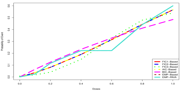
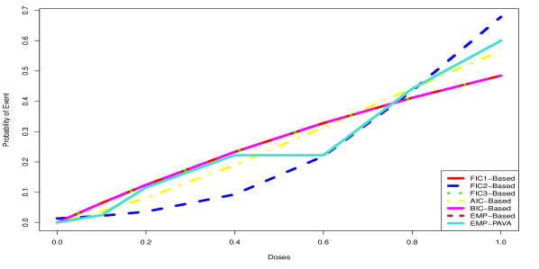
Figure 2: Connected lines of the estimated dose function evaluated at the standardized concentrations for the carcinogenecity data set provided by the different model selectors for BMR values of $0.01$ (top) and $0.10$ (bottom). Also included are the empirical probabilities and the PAVA estimates.

Table 6 provides the BMD estimates, under our standardized concentration scale, provided by the eight estimators described in Table 4. As expected, the estimation procedures for the BMD provide lower estimates at smaller BMRs. Note that the BMD estimates at BMR = .01 are close to each other except for that provided by the FIC3 method; while at BMR = .10 the estimate provided by FIC2 is drastically different from those of the other estimates. This is tied-in to the fact that at BMR = .10, the chosen model by FIC2, which is LG1, is highly different from the models chosen by the other methods; see the second panel in Figure 2. In the next section, we compare the performance of each of these BMD estimators with respect to their biases, standard errors, and root mean-square errors, under different scenarios via a modest simulation study.

Table 6: BMD estimates (in standardized concentrations) obtained by the eight estimators for the carcinogenecity data set for three different BMR values.

Estimator	BMR=0.01	BMR=0.05	BMR=0.1
FIC1	0.030	0.132	0.159
FIC2	0.030	0.132	0.442
FIC3	0.095	0.077	0.159
AIC	0.030	0.132	0.238
BIC	0.015	0.077	0.159
AICModAve	0.025	0.109	0.203
BICModAve	0.018	0.087	0.172
NONPAR	0.041	0.128	0.183

9 Simulation Studies

In order to compare the performance of the model selectors and BMD estimators illustrated in the Example, we performed a short series of computer simulation experiments. Our basic design for each simulation experiment was to generate dose-response data for a given set of $(N_{j},d_{j})$ values, $j=1,2,\ldots,J$, from a specific, true dose-response function $\pi(\cdot)$. For this data set, and over a range of BMR values, we obtained the selected model by each model selector and apply each BMD estimator just as in the Example above. This process was replicated ${\tt MREPS=2000}$ times. For these MREPS replications, we summarize the performance of the model selector by tabulating the number of times that it had chosen a given model class, and for the BMD estimators we obtain the mean, bias, standard error, and root mean-squared error. Note that we are able to compute the bias of each estimate since we know the exact BMD values under the true model for each BMR. The competing model classes utilized in the simulation coincide with those in the data illustration of Section 8.

9.1 Simulation Experiment #1

For the first simulation experiment, we used for our true data-generating model a multistage dose-response function of order $p=2$ (Model MS2 in Sec. 8) with $\beta$-coefficients given by

$$\mathbf{\beta}=(\beta_{0},\beta_{1},\beta_{2})=(0,0.32,0.52).$$

This choice is motivated by the estimated $\beta$-coefficients of the fitted model MS2 from the BCME carcinogenicity data example above. We also utilized the vector of doses from these data, given by

$$(d_{1},d_{2},\ldots,d_{7})=(0,0.1,0.2,0.4,0.6,0.8,1.0),$$

and vector of number of subjects, given by

$$(N_{1},N_{2},\ldots,N_{7})=(240,41,46,18,18,34,20).$$

The true simulation dose-response function is plotted in Figure 3.

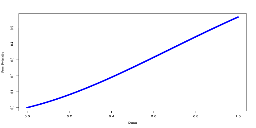
Figure 3: The true multistage dose-response function under Model MS2 for simulation experiment 1.

Figure 4 presents comparative boxplots of the BMD estimates obtained by the eight BMD estimators for BMRs of $0.01$ and $0.10$. Figures 5 and 6 present the corresponding bias and root mean-squared error plots for BMRs of $0.01$ and $0.10$. For additional resolution in the graphs, we also include results at BMR = $0.05$. Each of the curves are plotted as a function of BMR.

From the results of this particular simulation study, we observe that the BIC estimator underestimates the true BMD value, while the FIC3 estimator overestimates the true BMD value. The AIC Model-Averaged estimator, as well as the BIC Model-Averaged estimator, performed better than the others; with the AIC, FIC1, and PAVA-based Nonparametric estimators having comparatively mid-level performance. The BIC, FIC2, and FIC3 did not fare well relative to the other estimators.

With respect to the model selectors, from Table 7, we observe that the BIC model selector hardly chose the correct model, though both the AIC and BIC model selectors tended to choose the lower-order multistage model (MS1). The FIC1 model selector did quite well, as well as the FIC2 model selector. The FIC3 model selector did not also choose the correct model, and appeared undecided between the LG2 and MS1 models especially at BMR-values of 0.05 and 0.10. Note that the AIC and BIC selectors’ model choices do not vary with the BMR, whereas for the other three selectors the model choices do depend on the BMR value under consideration.

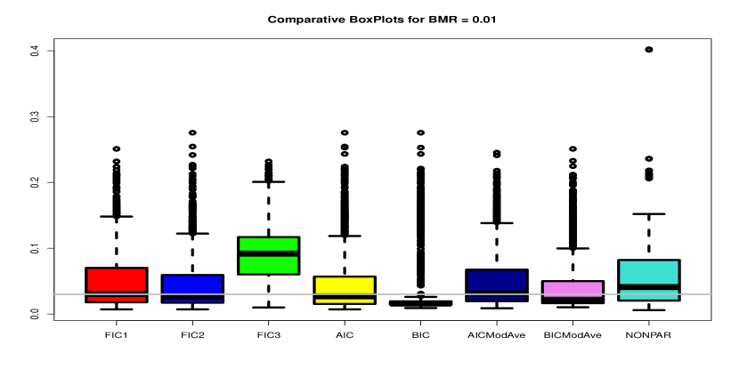
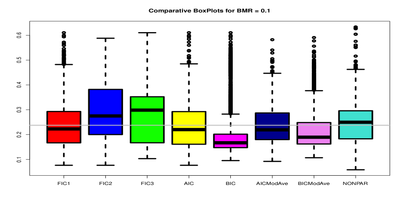
Figure 4: Comparative boxplots of the BMD estimates obtained by the eight different estimation schemes in simulation experiment #1 for BMR values $0.01$ (top) and $0.1$ (bottom). The gray horizontal line is the true BMD for the given BMR value. (Estimation scheme labels are given in Table 3.)

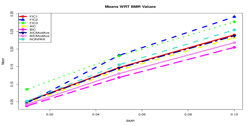
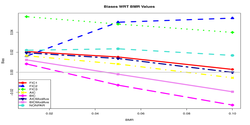
Figure 5: Bias plots of the eight BMD estimators for simulation experiment #1 for BMR values $0.01,0.05,0.1$. For each BMR and each estimator, the bias is the average of the differences between the BMD estimates and the true BMD value over the $2000$ simulations.

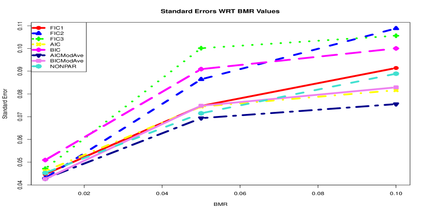
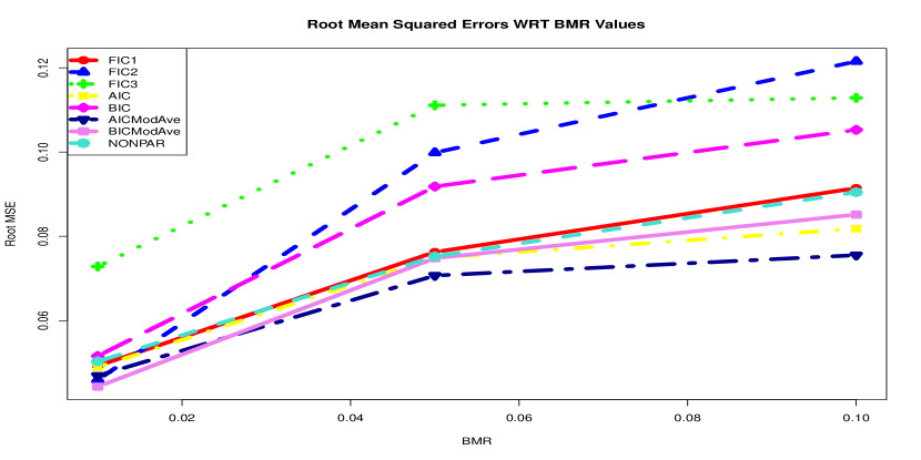
Figure 6: Root Mean-Square Error plots of the eight BMD estimators for simulation experiment #1 for BMR values $0.01,0.05,0.1$. For each BMR and each estimator, the Root Mean-Square Error is the average of the squared differences between the BMD estimates and the true BMD value over $2000$ simulations.

Table 7: Percentages of model selection by the five model selectors across the 2000 replications of Experiment #1. A multistage model of order 2 (MS2) is the true generating model, as described in Sec. 9.

Selector	BMR-Value	LG1	LG2	MS1	MS2
AIC	ALL	1.30	7.15	47.20	44.35
BIC	ALL	7.55	3.60	81.00	7.85
FIC1	0.01	11.15	2.10	18.35	68.40
FIC2	0.01	1.70	14.50	25.00	58.80
FIC3	0.01	24.35	52.20	23.45	0
FIC1	0.05	2.80	5.55	22.15	69.50
FIC2	0.05	9.55	27.90	10.10	52.45
FIC3	0.05	2.80	51.55	45.00	0.65
FIC1	0.10	5.95	6.40	31.35	56.30
FIC2	0.10	21.55	20.30	13.50	44.65
FIC3	0.10	6.60	48.55	37.00	7.85

9.2 Additional Experiments

We performed eight additional simulation experiments using different dose-response functions with varied shapes. The characteristics of each true generating model are provided in Table 8, where the true model parameters are determined by specifying the values of $\pi(\cdot)$ at two or three dose values. Notice that the true generating models in Experiments #2 to #5 have the same constraints on the smallest and largest doses, as do the models in Experiments #6 to #9. For each generating model we set $J=4$ doses with $(d_{1},d_{2},d_{3},d_{4})=(0,0.25,0.5,1)$ and $J=8$ doses with $(d_{1},d_{2},\ldots,d_{8})=(0,0.00625,0.03125,0.0625,0.125,0.25,0.50,1.00)$. The four-dose setting corresponds to a popular design in cancer risk experimentation [25], while the eight-dose setting expands upon this geometric spacing to focus on doses closer to the origin. Across the doses $d_{j}$, we took $N_{j}$ to be constant, i.e., $N_{j}=N$, and considered three different per-dose samples sizes: $N=50,100,1000$. The number of simulation replications remained ${\tt MREPS}=2000$. For Experiments #2 to #9, we present only the RMSE plots vs. BMR for $J=4$ doses and $N_{j}=100,j=1,2,\ldots,J$. These plots are given collectively in Figure 7. The percentages of selected models by all five model selectors for BMR values of $0.01$ and $0.1$ are presented in comparative bar plots given in Figure 8. Notice that the model selectors based on AIC and BIC remain independent of BMR, while the model selectors based on FIC1, FIC2, FIC3 differ.

Table 8: Characteristics of true generating models for additional simulation experiments.

Experiment	Model	Order	Constraint on the
Number	Class	$p$	True Dose-Response Function $\pi(\cdot)$
2	Logistic	1	$\pi(0)=0.05$, $\pi(1)=0.50$
3	Logistic	2	$\pi(0)=0.05$, $\pi(0.5)=0.30$, $\pi(1)=0.50$
4	Multistage	1	$\pi(0)=0.05$, $\pi(1)=0.50$
5	Multistage	2	$\pi(0)=0.05$, $\pi(0.5)=0.30$, $\pi(1)=0.50$
6	Logistic	1	$\pi(0)=0.30$, $\pi(1)=0.75$
7	Logistic	2	$\pi(0)=0.30$, $\pi(0.5)=0.52$, $\pi(1)=0.75$
8	Multistage	1	$\pi(0)=0.30$, $\pi(1)=0.75$
9	Multistage	2	$\pi(0)=0.30$, $\pi(0.5)=0.52$, $\pi(1)=0.75$

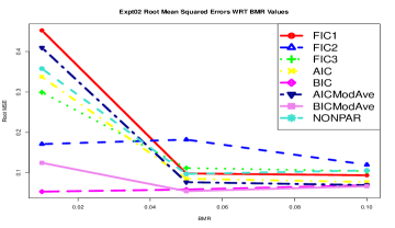
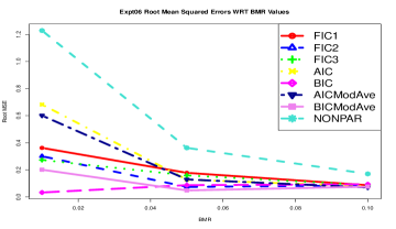
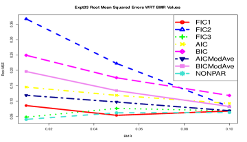
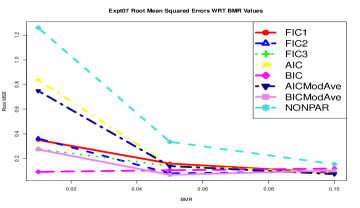
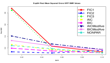
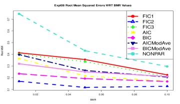
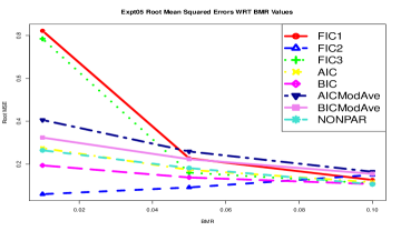
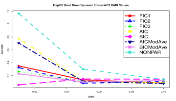
Figure 7: Simulated RMSE plots of the eight BMD estimators at BMR values of $0.01,0.05$ and $0.10$. Per-dose sample size is fixed at $N=100$ at each of $J=4$ doses. Plots from top left to bottom left and then top right to bottom right are for Experiments #2 to #9.

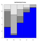
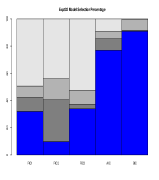
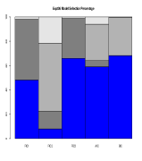
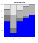
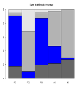
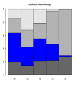
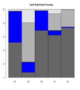
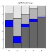
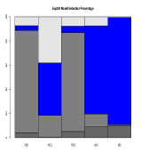
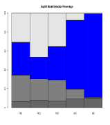
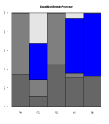
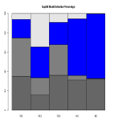
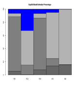
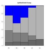
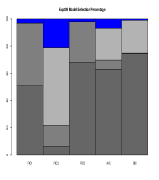
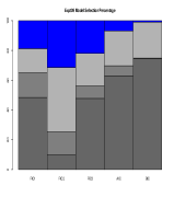
Figure 8: Comparative bar charts of the five model selectors from table 4. Successive portions from bottom to top in each vertical position in a plot frame depict percentages that model classes LG1, LG2, MS1, and MS2 were selected, with the five vertical positions from left to right associated with selectors FIC1, FIC2, FIC3, AIC, and BIC. Blue bars correspond to the correct models. The two plot frames in each plot panel are for BMR $=0.01$ (left) and $0.10$ (right). The eight plot panels going from top left to bottom left then top right to bottom right are for Experiments #2 to #9.

Examining Figure 7 and Figure 8, we find that the eight BMD estimators and five model selectors exhibit varied performance among the eight simulation experiments. None of these estimators and model selectors could be said to totally dominate the others. The BIC-based estimators appeared to possess the most stable performance over the three BMR values. In essence, which estimator performs best depended to a large extent on the shape of the true dose-response function. Generally, the FIC2 and BIC-based estimators tended to perform similarly, whereas the FIC1, FIC3, AIC-based, and the nonparametric estimators tended to have comparable RMSE plot patterns. It is also interesting to note that the BIC-model averaged estimators did not always dominate the BIC-two step estimator, and the same could be said for the AIC-based estimators, though for the latter the RMSEs tended to be closer. Surprisingly, the FIC2 estimator appeared to perform well when the true model class is multistage, and poorly when the true model class is logistic. This could be because the FIC2 model selector tended to choose the multistage model class (cf. Figure 8). Also, we note that the AIC and BIC model selectors tended to choose lower-order models, as expected [20], though not necessarily lower-order models in the true model class. More importantly, we call attention to the fact that the BIC model selector hardly ever chose the correct model class when the true model class is multistage of order 2 (MS2), but at the same time its associated BMD estimators performed quite well in terms of RMSE! This seems to indicate that, perhaps, in the context of estimating relevant parametric functionals when there are several competing model classes, it is not so crucial that the model selector involved in two-step procedures be able to choose the correct model, but rather that its associated parameter estimator perform well in estimating the functional of interest.

10 Concluding Remarks

This paper has provided several strategies for estimating the benchmark dose (BMD) in quantal-response studies when the dose-response function may be thought to belong to several competing model classes. Two-stage type procedures, wherein a model is first chosen and then an estimate is obtained within the chosen model, are described as arising from the most common information measures, the AIC and BIC, and also from a focused-inference approach which relies centrally on the Kullback-Leibler divergence. Model-averaging type procedures are also described, which are characterized by combining estimates from the different model classes according to appropriate data-dependent weights.

The model selection procedures and BMD estimators are illustrated using a carcinogenecity data set. Through simulation studies, the performance of the different model selectors and BMD estimators are compared. A nonparametric BMD estimator based on an empirical estimator of the dose-response function obtained by applying the pooled-adjacent-violators algorithm (PAVA) on the empirical probabilities at each dose level [24] was also included among the estimators that were compared. An interesting phenomenon is that with two-step procedures, in order for the BMD estimator to perform well in terms of RMSE, it does not appear imperative for the associated model selector to be able to choose with high probability the true generating model. This was particularly evident with the BIC-based procedures where the BIC model selector did not perform well with respect to choosing the true generating model, but its associated BMD estimators, both in two-step and model-averaged versions, exhibited competitive RMSEs. Of course it should be recognized that the limited simulation study we have performed is insufficient to make truly definitive conclusions. Clearly, further examinations and comparisons of these different model selectors and BMD estimators are warranted to obtain more definitive conclusions, especially when there are more than two model types.

Finally, we emphasize further that extreme caution is called-for when assessing the properties of estimates, where ‘double-dipping’ of the data leads to inferential instabilities. In particular, additional studies will be needed to ascertain the impact of model selection on the distributional properties. For instance, the standard errors of the resulting BMD estimators, or small-sample coverage of any confidence regions based on these estimators, will be important to determine; see, for instance, the recent papers by [34] and [22]. Such results will have important bearing in the construction of statistical inferences on the BMD.

References

• [1] H. Akaike. Information theory and an extension of the maximum likelihood principle. In Second International Symposium on Information Theory (Tsahkadsor, 1971), pages 267–281. Akadémiai Kiadó, Budapest, 1973.
• [2] A. John Bailer, R. B. Noble, and M. W. Wheeler. Model uncertainty and risk estimation for experimental studies of quantal responses. Risk Analysis, 25:291–299, 2005.
• [3] Brooke E. Buckley, Walter W. Piegorsch, and R. Webster West. Confidence limits on one-stage model parameters in benchmark risk assessment. Environmental and Ecological Statistics, 16:53–62, 2009.
• [4] Kenneth P. Burnham and David R. Anderson. Model selection and multimodel inference: a practical information-theoretic approach. Springer-Verlag, New York, second edition, 2002.
• [5] Joseph E. Cavanaugh. A large-sample model selection criterion based on Kullback’s symmetric divergence. Statist. Probab. Lett., 42(4):333–343, 1999.
• [6] Gerda Claeskens and Nils Lid Hjort. The focused information criterion. J. Amer. Statist. Assoc., 98(464):900–945, 2003. With discussions and a rejoinder by the authors.
• [7] Gerda Claeskens and Nils Lid Hjort. Model Selection and Model Averaging. Cambridge Series in Statistical and Probabilistic Mathematics. Cambridge University Press, Cambridge, 2008.
• [8] R. C Deutsch, J. M. Grego, B. T. Habing, and Walter W. Piegorsch. Maximum likelihood estimation with binary-data regression models: small-sample and large-sample features. Advances and Applications in Statistics, 14(2):101–116, 2010.
• [9] Vanja M. Dukić and Edsel A. Peña. Variance estimation in a model with Gaussian submodels. J. Amer. Statist. Assoc., 100(469):296–309, 2005.
• [10] C. Faes, M. Aerts, H. Geys, and G. Molenberghs. Model averaging using fractional polynomials to estimate a safe level of exposure. Risk Analysis, 27:111–123, 2007.
• [11] Nils Lid Hjort and Gerda Claeskens. Frequentist model average estimators. J. Amer. Statist. Assoc., 98(464):879–899, 2003.
• [12] J. Hoeting, D. Madigan, A. Raftery, and C. Volinsky. Bayesian model averaging. Statistical Science, 14:382–401, 1999.
• [13] Clifford M. Hurvich and Chih-Ling Tsai. Regression and time series model selection in small samples. Biometrika, 76(2):297–307, 1989.
• [14] M. Hwang, E. Yoon, J. Kim, D. D. Jang, and T. M. Yoo. Toxicity value for 3-monochloropropane-1,2-diol using a benchmark dose methodology. Regulatory Toxicology and Pharmacology, 53:102–106, 2009.
• [15] M. Kuschner, S. Laskin, R.T. Drew, V. Cappiello, and N. Nelson. Inhalation carcinogenicity of alpha halo ethers. iii. lifetime and limited period inhalation studies with bis(chloromethyl)ether at 0.1 ppm. Arch. Environ. Health, 30(2):73–77, 1975.
• [16] E. L. Lehmann and George Casella. Theory of point estimation. Springer Texts in Statistics. Springer-Verlag, New York, second edition, 1998.
• [17] Michael A. Messig and William E. Strawderman. The asymptotic behaviour of Bayes estimators for dichotomous quantal response models. Sankhyā Ser. A, 60(3):418–425, 1998.
• [18] Knashawn H. Morales, Joseph G. Ibrahim, Chien-Jen Chen, and Louise M. Ryan. Bayesian model averaging with applications to benchmark dose estimation for arsenic in drinking water. J. Amer. Statist. Assoc., 101(473):9–17, 2006.
• [19] B. J. T. Morgan. Analysis of Quantal Response Data. Chapman & Hall, New York, 1992.
• [20] A. A. Neath and J. E. Cavanaugh. The Bayesian information criterion: background, derivation, and applications. Wiley Interdisciplinary Reviews: Computational Statistics, 4(2):199–203, 2012.
• [21] Daniela Nitcheva, Walter W. Piegorsch, and R. Webster West. On use of the multistage dose-response model for assessing laboratory animal carcinogenicity. Regul. Toxicol. Pharmacol., 48:135–147, 2007.
• [22] Walter W. Piegorsch, Lingling An, Alissa A. Wickens, R. Webster West, Edsel A. Peña, and Wensong Wu. Information-theoretic model-averaged benchmark dose analysis in environmental risk assessment. Environmetrics, 24(3):143–157, 2013.
• [23] Walter W. Piegorsch and A. John Bailer. Analyzing Environmental Data. John Wiley & Sons, Chichester, 2005.
• [24] Walter W. Piegorsch, Hui Xiong, Rabi N. Bhattacharya, and Lizhen Lin. Nonparametric estimation of benchmark doses in environmental risk assessment. Environmetrics, 23(8):717–728, 2012.
• [25] C. J. Portier. Biostatistical issues in the design and analysis of animal carcinogenicity experiments. Environmental Health Perspectives, 102, Suppl. 1:5–8, 1994.
• [26] R Development Core Team. R: A Language and Environment for Statistical Computing. R Foundation for Statistical Computing, Vienna, Austria, 2011.
• [27] Tim Robertson, F. T. Wright, and R. L. Dykstra. Order restricted statistical inference. Wiley Series in Probability and Mathematical Statistics: Probability and Mathematical Statistics. John Wiley & Sons Ltd., Chichester, 1988.
• [28] S. Sand, A. FalkFilipsson, and K. Victorin. Evaluation of the benchmark dose method for dichotomous data: Model dependence and model selection. Regulatory Toxicology and Pharmacology, 36:184–197, 2002.
• [29] S. Sand, K. Victorin, and A. FalkFilipsson. The current state of knowledge on the use of the benchmark dose concept in risk assessment. Journal of Applied Toxicology, 28:405–421, 2008.
• [30] G. Schwartz. Estimating the dimension of a model. Ann. Statist., 6:461–464, 1978.
• [31] K. Shao and M. J. Small. Potential uncertainty reduction in model-averaged benchmark dose estimates informed by an additional dose study. Risk Analysis, 31:1561–1575, 2011.
• [32] K. Takeuchi. Distribution of informational statistics and a criterion of model fitting (in Japanese). Suri-Kagaku (Mathematical Sciences), 153:12–18, 1976.
• [33] U.S. EPA. Benchmark dose technical guidance document: Technical Report No. EPA/100/R-12/001. U.S. Environmental Protection Agency, Washington, DC, 2012.
• [34] R. Webster West, Walter W. Piegorsch, Edsel A. Peña, Lingling An, Wensong Wu, Alissa A. Wickens, Hui Xiong, and Wenhai Chen. The impact of model uncertainty on benchmark dose estimation. Environmetrics, 23(8):706–716, 2012.
• [35] M. W. Wheeler and A. John Bailer. Properties of model-averaged BMDLs: A study of model averaging in dichotomous response risk estimation. Risk Analysis, 27:659–670, 2007.
• [36] M. W. Wheeler and A. John Bailer. Comparing model averaging with other model selection strategies for benchmark dose estimation. Environmental and Ecological Statistics, 16:37–51, 2009.
• [37] Arnold Zellner and Peter E. Rossi. Bayesian analysis of dichotomous quantal response models. J. Econometrics, 25(3):365–393, 1984.