Coupled Spin and Shape Evolution of Small Rubble-Pile Asteroids: Self-Limitation of the YORP Effect

Abstract

We present the first self-consistent simulations of the coupled spin-shape evolution of small gravitational aggregates under the influence of the YORP effect. Because of YORP’s sensitivity to surface topography, even small centrifugally driven reconfigurations of aggregates can alter the YORP torque dramatically, resulting in spin evolution that can differ qualitatively from the rigid-body prediction. One third of our simulations follow a simple evolution described as a modified YORP cycle. Two-thirds exhibit one or more of three distinct behaviors—stochastic YORP, self-governed YORP, and stagnating YORP—which together result in YORP self-limitation. Self-limitation confines rotation rates of evolving aggregates to far narrower ranges than those expected in the classical YORP cycle, greatly prolonging the times over which objects can preserve their sense of rotation. Simulated objects are initially randomly packed, disordered aggregates of identical spheres in rotating equilibrium, with low internal angles of friction. Their shape evolution is characterized by rearrangement of the entire body, including the deep interior. They do not evolve to axisymmetric top shapes with equatorial ridges. Mass loss occurs in one-third of the simulations, typically in small amounts from the ends of a prolate-triaxial body. We conjecture that YORP self-limitation may inhibit formation of top-shapes, binaries, or both, by restricting the amount of angular momentum that can be imparted to a deformable body. Stochastic YORP, in particular, will affect the evolution of collisional families whose orbits drift apart under the influence of Yarkovsky forces, in observable ways.

1 Introduction

The distribution of asteroids with diameters larger than a few hundred meters in the period-diameter diagram is interpreted widely as evidence that these objects are not monolithic boulders (Davis et al. 1979, Harris 1996). The sharp cutoff in rotation period at $P\approx 2\mbox{$\rm\,h$}$ matches the spin rate at which material at the equator of a rocky sphere would become gravitationally unbound; the persistence of this envelope to large sizes implies that these objects are dominated by gravity, obscuring the effects of tensile or shear strength (Holsapple 2007). Their actual structures may range from contact configurations of a few monolithic blocks to nearly homogeneous collections of individual small grains. Direct measurements of the masses and volumes of 433 Eros and 25143 Itokawa by the NEAR-Shoemaker and Hayabusa spacecraft imply porosities of 27% (Wilkison et al. 2002) and 40% (Abe et al. 2006), respectively, arguing for both fractured bodies and genuine rubble piles in the near-Earth asteroid (NEA) population.

In sharp contrast, NEAs smaller than about $150\mbox{$\rm\,m$}$ in diameter overwhelmingly are rotating faster than the $2\mbox{$\rm\,h$}$ limit. These objects are under centrifugal tension in directions perpendicular to the spin axis, and under gravitational compression along it. Despite an initial rush to dub them “monolithic fast rotators,” it was shown by Holsapple (2007) that geological granular materials can supply sufficient cohesion to hold aggregate bodies together at the observed sizes and spin rates. The most surprising aspect of the fast-rotating asteroids (FRAs) is their abrupt appearance as a function of absolute magnitude: essentially everything smaller than $H=23.6$ (nominal diameter $\sim 60\mbox{$\rm\,m$}$), and nothing larger than $H=21.4$ ($\sim 170\mbox{$\rm\,m$}$), is a fast rotator (Statler et al. 2013). This abrupt transition is not predicted by current strength models (Holsapple 2007, Sánchez and Scheeres 2014).

Owing to the action of the YORP effect—the secular torque due to the reflection and thermal re-emission of solar radiation from the surface (Paddack 1969, Rubincam and Bottke 2000, Rubincam 2000, Bottke et al. 2006)—the current spins of NEAs with diameters ($D$) of a few km or smaller may not reflect their original spin states. YORP spin timescales $|P/(dP/dt)|$ in the inner Solar System are $\sim 10^{6}(D/1\mbox{$\rm\,km$})^{2}\mbox{$\rm\,yr$}$ (Rubincam 2000), as confirmed by observational detections of YORP acceleration (Lowry et al. 2007, Taylor et al. 2007, Kaasalainen et al. 2007, Durech et al. 2008a; b, Ďurech et al. 2012, Lowry et al. 2014). Typical NEA lifetimes are $\sim 10^{7}\mbox{$\rm\,yr$}$ (Gladman et al. 1997), so there is ample opportunity, in principle, for YORP to modify the spins of sub-km-sized NEAs.

For a given object and orbit, the secular YORP torque is a fixed vector function of obliquity. It has become standard practice to use the plot of the torque components vs. obliquity—the “YORP curves”—as a description of the YORP characteristics of an object. If the object remains rigid, the YORP curves determine its spin evolution: the so-called “YORP cycle” (Rubincam and Bottke 2000). A typical cycle begins with the object at an obliquity at which the torque component along the spin axis is positive; the object accelerates in spin rate and evolves in obliquity until it reaches an orientation at which the spin component changes sign, then decelerates while evolving toward an end-state obliquity that is a stable fixed point. Once the spin period is comparable to the orbital period, spin-orbit resonances come into play; these, along with tides or small impacts, randomly re-orient the rotation axis, possibly after an episode of slow chaotic tumbling, to an obliquity at which the cycle can begin anew.

The YORP cycle concept has important implications for orbital evolution driven by the Yarkovsky effect (the net radiation recoil force), which itself is spin-state dependent. Most NEAs are thought to have been delivered from the Main Belt to their current orbits with retrograde rotation, having drifted inward (via Yarkovsky) to various resonances (Bottke et al. 2002, La Spina et al. 2004). Once in the inner Solar System, YORP timescales should become short. As the asteroids complete their YORP cycles, their previous spin states would be forgotten, and the preference for retrograde rotation should be erased. Yet, recent observational determinations of Yarkovsky semi-major axis drift rates from available radar and optical astrometry find that the overwhelming majority have $da/dt<0$, indicating retrograde rotation (Chesley et al. 2008, Nugent et al. 2012, Farnocchia et al. 2013). This is difficult to reconcile with simple time-scale arguments showing that YORP should have been able to re-write the spin state distribution of sub-km-sized objects many times over.

The possibility that the YORP cycle may accelerate objects to high rotation rates has excited interest in spin-driven reshaping and binary formation, a compelling demonstration of which is presented by Walsh et al. (2008). These authors simulate idealized self-gravitating aggregate asteroids composed of identical spheres, assumed to be inexorably accelerated by YORP. They find that the objects with a suffciently high internal angle of friction, or with a rigid core, become oblate and develop an equatorial ridge, making the body resemble a child’s top. Continued spin-up causes the ridge to shed material, which can then reaccrete in orbit. This process dynamically associates binaries with top shapes; and the strong resemblance of the simulated binary formed by Walsh et al. (2008) to the actual binary 1999 KW₄ (Ostro et al. 2006) is striking. YORP is now widely held to be an important mechanism in binary formation. But this belief rests on the assumption that YORP will, first, accelerate objects to spin rates high enough to form axisymmetric tops; then, accelerate the tops so that they shed mass; and finally, drive sufficient mass off the surface and into orbit to form a binary companion. Simulations to date have adopted the ansatz that YORP will provide angular momentum in whatever amount is needed to accomplish this. But this is not a safe assumption when the object is not a rigid body.

Deformability, as one would expect for a rubble pile, fractured body, or anything with loose surface material, may significantly alter the behavior of the YORP effect. Because the net YORP torque is a small residual of an imperfect cancellation of competing contributions across the asymmetric surface, YORP is inherently sensitive to the internal mass distribution and to the detailed surface topography. Scheeres and Gaskell (2008) demonstrated that $\sim 50\mbox{$\rm\,m$}$ shifts of 25143 Itokawa’s center of mass could change the sign of the spin component of torque, an effect subsequently confirmed by Lowry et al. (2014). Statler (2009) systematically studied the topographic effect on a wide variety of simulated asteroids, and showed that objects that are identical but for the location of a single crater or boulder can have torques differing by factors of several. Statler (2009) further conjectured that the successive effects of minor structural changes that alter the surface may qualitatively alter spin evolution under YORP, possibly replacing the YORP cycle with a stochastic random walk at rotation periods $\lesssim 10\mbox{$\rm\,h$}$, and potentially limiting the amount of angular momentum that YORP can contribute to processes like rotational reshaping and binary formation.

The purpose of this paper is to test the conjecture of Statler (2009) through self-consistent numerical simulations of coupled shape and spin evolution of gravitationally bound aggregates driven by the YORP effect. We will demonstrate that stochastic YORP can, indeed, occur, and is just one of three distinct processes deriving from spin-driven shape change, that collectively give rise to YORP self-limitation. Section 2 describes our numerical approach and the simulated aggregates that we use for our initial conditions. Section 3 presents the results, describing the time evolution in spin and obliquity as well as the statistics of mass reconfigrations, shape changes, and mass shedding; it also presents a preliminary version of a statistical (Monte Carlo) description of self-consistent spin evolution. Section 4 discusses the implications for top shapes, binaries, and the Yarkovsky effect, and Section 5 sums up.

2 Numerical Methods

2.1 Overview

The physical system we are simulating is characterized by two very different timescales: the dynamical timescale—$10^{3}\mbox{$\rm\,s$}$ to $10^{5}\mbox{$\rm\,s$}$—on which the object rotates and centrifugally driven material movement may occur, and the YORP timescale—$10^{13}\mbox{$\rm\,s$}$ to $10^{15}\mbox{$\rm\,s$}$ for kilometer-sized objects—on which the spin state is altered. Running a discrete-element simulation for $10^{10}$ dynamical times is not feasible, but we can exploit the difference in timescales. Material reconfigurations, quick compared with the YORP timescale, take place at effectively constant angular momentum; and YORP evolution, acting slowly between reconfigurations, takes place at constant shape. This allows us to adopt a two-step computational approach in which we integrate the YORP-induced spin state evolution at constant shape, incrementing (or decrementing) the spin rate in the discete-element code on a greatly compressed timescale until material movement is triggered, and then follow the dynamical evolution in “real” time, at constant angular momentum, until the reconfiguration is finished. At that point we recompute the torques for the new shape and resume the spin state integration. This back-and-forth approach, handing off between the particle dynamics and the radiation dynamics parts of the calculation, is the key to making these simulations possible.

2.2 Gravity and Particle Dynamics: pkdgrav

The gravitational and particle dynamics are simulated using the hard-sphere discrete element method (HSDEM) as implemented in pkdgrav, a gravitational $N$-body tree code originally developed for cosmology (Stadel 2001) and subsequently modified to handle interparticle collisions (Richardson et al. 2000; 2009; 2011). The ensemble of spherical particles used by pkdgrav is intended to model the collective behavior of a deformable material composed of discrete pieces, not to literally represent components of the aggregate. Collisions between pairs of spheres are treated as instantaneous events that alter their translational and rotational motions. Dissipative effects are parametrized by coefficients of restitution that affect the relative motion of the surfaces at the point of contact in the normal ($\varepsilon_{n}$) and tangential ($\varepsilon_{t}$) directions. To avoid an unmanageable number of extremely low-velocity collisions, $\varepsilon_{n}$ and $\varepsilon_{t}$ are set to 1 (no dissipation) below a threshhold controlled by two additional parameters termed the collapse limit and the slide limit. Because dissipative processes in small asteroids are not quantitatively well understood, we do not attempt at this stage to model the rate of relaxation or the lifetimes of non-principal-axis (NPA) rotation states. Cohesive forces can, in principle, be included, but are ignored in the simulations reported here; hence the results are applicable to objects in the few-kilometer size range where gravity dominates, and are not easily scalable to smaller sizes where cohesion is expected to become relatively more important.

Aggregates modeled by the HSDEM approach may be somewhat more deformable than real aggregates composed of irregularly shaped components, owing to the ability of the spherical particles to roll. The use of identical spheres allows for a certain degree of rigidity resulting from “cannonball stacking”. Richardson et al. (2005) and Walsh et al. (2012) find that cannonball-stacked arrangements of identical spheres in hexagonal-close-pack (HCP) configuration have angles of friction near $40\arcdeg$, comparable to lunar and martian regolith. When the spheres are not in ordered packing, the resulting aggregates have angles of friction in the range of $5\arcdeg$ to $10\arcdeg$. This is lower than typical values for terrestrial granular materials; however, the properties of real asteroidal materials are not quantitatively well determined. Tanga et al. (2009), using the pkdgrav HSDEM implementation, demonstrate that a population of disordered aggregates of identical spheres, allowed to equilibrate at constant angular momentum, can collectively reproduce the observed asteroid shape distribution. On the basis of this result we adopt the objects from the Tanga et al. (2009) study as our test objects in this paper. These choices represent a simple starting point, a first step in simulations of self-consistent spin evolution. In Section 4 we describe physical mechanisms and computational strategies that will be appropriate for subsequent steps.

2.3 Radiation and Surface Physics: TACO

The dynamical effects of radiation recoil are calculated using TACO (Statler 2009), a code for calculating thermophysical processes on the surfaces of inactive small bodies. TACO models an asteroid surface using a triangular tiling. The interaction of each tile with incident solar radiation is described by a Hapke model for the bidirectional reflectance (Hapke 2002). Shadowing is handled explicitly by calculating a horizon map for each tile, which gives the maximum elevation of the visible parts of the surface as a function of azimuth from the tile centroid. The incident radiation that is not reflected is absorbed and heats the surface. TACO includes the ability to solve the 1-dimensional heat conduction equation for the flow of heat into and out of the surface; however, for computational expediency in these simulations we work in the limit of zero thermal inertia, so that the absorbed radiation is instantaneously re-emitted. Non-zero thermal inertia changes the obliquity torques, but not the spin torques, so this simplification is a reasonable strategy for obtaining statistically representative descriptions of spin evolution. The thermal emission is assumed to be Lambertian (i.e., isotropic into the sky hemisphere), with a correction for partial blockage of the sky by an elevated horizon (Statler 2009). The code computes the torques from both the reflected and emitted radiation, though the latter dominates for typically dark asteroids.

2.4 Self-Consistent Spin and Shape Evolution

In order to self-consistently model the spin and shape evolution, we developed four additional code elements that work with pdkgrav and TACO, and carry out the following tasks:

1. Fit a triangular tiling over a pkdgrav object composed of spheres, to pass to TACO for computing the YORP torques;

2. Identify when a movement of material has occured, and minimally adjust the tiling to accommodate the movement (leaving it unchanged over the part of the surface where no movement occurred);

3. Integrate the spin and obliquity in time using the torques calculated by TACO; and finally,

4. Orchestrate the entire procedure, running and passing data between the codes.

We describe each of these elements in detail below.

2.4.1 Tiling

Our initial test objects (Section 2.5) are aggregates of identical spheres. To fit a tiling over an object, we first compute and diagonalize the intertia tensor, and rotate the object to principal axis orientation with the center of mass at the origin and the $x$, $y$, and $z$ axes corresponding to the long, middle, and short axes, respectively. We then create a tiling of the equivalent ellipsoid with the same bulk density. At this point the ellipsoidal tiling is close to the object, and the goal is to adjust the vertices to fit the tiling tightly around it. We define the function

$$G(x,y,z)\equiv R^{2n}\sum_{j=1}^{N}\left[(x-x_{j})^{2}+(y-y_{j})^{2}+(z-z_{j})^{2}\right]^{-n}-G_{0},$$ (1)

where $R$ is the sphere radius, $(x_{j},y_{j},z_{j})$ are the coordinates of the center of sphere $j$, $N$ is the number of spheres, and $n$ and $G_{0}$ are constants chosen so that the surface $G(x,y,z)=0$ tightly surrounds the object. We have found by trial and error that the choice $n=2$ and $G_{0}=1.25$ works well for a variety of aggregate shapes. Each vertex of the ellipsoidal tiling is moved in or out in the direction normal to the ellipsoid, to place it on the surface $G(x,y,z)=0$ as shown in Fig. 1. Finally, the tiling is rotated back to the orientation of the original object.

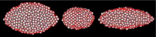
Figure 1: Othogonal views of an aggregate of spheres along with the triangular tiling in red, projected onto the (left) $xy$ plane, (center) $yz$ plane, (right) $xz$ plane.

One should remember that both the system of spheres and the triangular tiling are numerical idealizations. They are intended to simulate the collective behavior of a real aggregate composed of irregular rocks, pebbles, and regolith, not to literally represent the constituent pieces. Hence there is no need to resolve each sphere individually with an extremely fine mesh, or to resolve each surface facet by filling the interior with tiny spheres.

Nonetheless, Statler (2009) emphasized the extreme sensitivity of YORP to the detailed topography of asteroid surfaces. So we should be concerned about the sensitivity of the computed torques in our simulations both to the resolution of the tiling and to the positioning of the tiling on the aggregate object. We have tested this by calculating the torques on a small selection of aggregates at 9 different resolutions (determined by the number of tiles, ranging from 784 to 19,960) and small angular shifts of the tilings (by a few degrees). As expected, we find that the torque vaires typically by tens of percent among the various shifts and resolutions. This result implies that the exact results of our simulations will depend on arbitrary choices of parameters related to the resolution and tiling. We adopt the lowest resolution consistent with the number of spheres in the initial objects, and stress that the detailed results of each simulation will be resolution-dependent, and should be interpreted only as examples of the types of behavior that may result from self-consistent YORP.

2.4.2 Detecting Material Movement and Updating the Tiling

We define a movement of material as a shift of one or more pkdgrav spheres by more than a quarter of its radius. To determine whether a movement has occurred, we compare the current object with the object resulting from the previous movement. If no spheres have moved, the current object should be a rotated and translated copy of the earlier object, except for small differences caused by the slight bouncing of spheres that is inherent in the HSDEM approach. We use the LMDIF routine from the MINPACK (Moré et al. 1984) library to fit for the three Euler angles and three displacements describing the rotation and translation that minimizes the sum of the squares of the differences in sphere positions. After the initial fit, the spheres that have moved by more than the allowed tolerance are flagged and excluded, and the fit is obtained again. The process is iterated until none of the remaining spheres is flagged as having moved. Figure 2 shows an example of two consecutive objects, with the spheres identified as having moved marked with black spots.

When a material movement has occurred, we need to update the tiling. However, we must ensure that, insofar as is possible, the tiling is altered only over the regions where motion occurred, so that any changes to the YORP torques are due to the motion itself and are not merely the result of a shifted tiling. To “minimally evolve” the tiling, we transform the new object back to the original orientation at time $t=0$, and re-build the tiling starting from the original equivalent ellipsoid. This guarantees that those spheres that do not move will be at the same position that they were initially and therefore will receive the same tiling. Figure 2 shows the tilings on the example objects before and after material motion.

Our minimal evolution algorithm can encounter difficulties when an initially flattened or elongated object becomes significantly rounder. As described below, this limits the simulations to objects with intitial flattenings $c/a>0.5$.

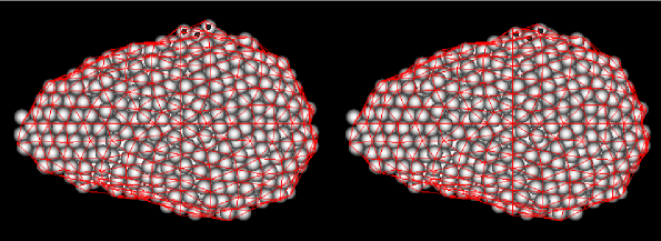
Figure 2: Showing the adjustment of the tiling on an aggregate object before (left) and after (right) a small movement of material. The line of sight is along the spin axis. The tiling is shown in red. Black asterisks identify 3 spheres that move by more than a quarter of the sphere’s radius. Note that after the movement the tiling has been modified in that area while remaining unchanged elsewhere.

2.4.3 Spin-State Evolution

The rate of change of the obliquity $\epsilon$ and the angular velocity $\omega$ are given by (Rubincam 2000)

$$\frac{d\epsilon}{dt}=\frac{T_{\epsilon}}{C\omega}$$ (2)

and

$$\frac{d\omega}{dt}=\frac{T_{\omega}}{C}$$ (3)

where $C$ is the moment of inertia about the rotation axis and $T_{\epsilon}$ and $T_{\omega}$ are spin- and orbit-averaged torque components, respectively: $T_{\omega}$ is the component parallel to the spin axis, and $T_{\epsilon}$ is the orthogonal component that lies in the plane containing both the spin axis and the orbit normal. Once a tiling is obtained for a given object, $T_{\epsilon}$ and $T_{\omega}$ are calculated using TACO over an obliquity grid with a spacing of $5\arcdeg$. At intermediate values of obliquity, the torques are interpolated from the grid. Equations (2) and (3) are solved numerically using a fourth-order Runge Kutta integrator with a $10^{3}$ year step size. We have verified that this routine reproduces the exact analytic results for idealized cases of rigid-body evolution in which the YORP curves take the forms $T_{\omega}\propto\cos\epsilon$ and $T_{\epsilon}\propto\sin\epsilon$.

2.4.4 Orchestrating the Simulations

Top-level control of the simulations is handled by a python script that orchestrates the back-and-forth stepping between TACO and pkdgrav and enables their interaction with the additional routines described above. Details of the logic, including a flowchart showing the individual steps, are given in the Appendix.

2.5 Initial Conditions

We select our initial test objects from a collection of 144 rotating equilibria created using pkdgrav (Tanga et al. 2009). These authors built ellipsoidal aggregates with various shapes and initial spins, and then allowed them to evolve and reconfigure dynamically until they reached stable configurations. The objects have a natural disordered packing, and are composed of 1000 spheres of radius $50.2\mbox{$\rm\,m$}$, each with density of $2.96\mbox{$\rm\,g$}\mbox{$\rm\,cm$}^{-3}$. The bulk densities and mean diameters are in the range of $1.55$ to $1.72\mbox{$\rm\,g$}\mbox{$\rm\,cm$}^{-3}$ and $1.3$ to $2.0\mbox{$\rm\,km$}$, respectively. We tile each object, compute the torques, and integrate the spin state evolution it would undergo if it remained rigid. We intentionally pick objects that, were they rigid bodies, would initially accelerate in spin rate and display a representative range of YORP-cycle behaviors. In particular, we select four objects that would spin up at all obliquities, with rigid-body end states in which (formally) $\omega\to\infty$ as $t\to\infty$. The remaining 12 objects are chosen to be approximately uniformly distributed in the axis-ratio plane, subject to the requirement that $c/a\geq 0.5$ to avoid numerical difficulties in minimally evolving the tiling.

Table 1 shows the initial parameters for our sample of 16 aggregates. Figure 3 shows the initial distribution of shapes in the axis-ratio plane, plotted in terms of the short-to-long axis ratio ($c/a$) and the triaxiality parameter $T$, defined by

$$T\equiv{{1-(b/a)^{2}}\over{1-(c/a)^{2}}}.$$ (4)

Objects with $T=0$ are oblate spheroids ($b=a$), and those with $T=1$ are prolate spheroids ($b=c$). The initial distribution is representative of the distribution of known asteroid shapes approximated by triaxial ellipsoids (Tanga et al. 2009, Kryszczyńska et al. 2007).

Table 1: Initial Aggregate Objects

Simulation	Semi-axis ratio		Semi-major axis $a$	Bulk Density	Period
	$b/a$	$c/a$	(km)	($\mbox{$\rm\,g$}\mbox{$\rm\,cm$}^{-3}$)	(hours)
1	0.91	0.88	0.686	1.55	10.08
2	0.88	0.87	0.696	1.66	10.00
3	0.94	0.83	0.688	1.62	10.51
4	0.86	0.74	0.722	1.62	15.52
5	0.88	0.82	0.701	1.66	10.34
6	0.78	0.69	0.765	1.66	15.72
7	0.70	0.70	0.797	1.66	15.74
8	0.74	0.65	0.799	1.63	16.09
9	0.77	0.62	0.786	1.67	16.26
10	0.99	0.76	0.698	1.61	15.70
11	0.97	0.89	0.672	1.72	15.00
12	0.51	0.50	1.000	1.60	15.28
13	0.68	0.55	0.871	1.56	14.54
14	0.59	0.53	0.935	1.55	14.84
15	0.78	0.59	0.795	1.68	14.35
16	0.92	0.64	0.745	1.63	14.19

Figure 3: The semi-axis ratio distribution of the initial shapes, plotted in terms of the short axis ratio $c/a$ and the triaxiality parameter $T\equiv[1-(b/a)^{2}]/[1-(c/a)^{2}]$. Purely oblate objects have $T=0$ and purely prolate objects have $T=1$.

We dynamically evolve the initial objects with pkdgrav for several rotations to ensure that all mass motion has stopped. We then recompute the initial tilings and torques, and again consider the rigid body evolution of the fully settled objects. We choose initial obliquities so that, if they remained rigid, the objects would evolve through a wide range of obliquities and spin rates. The adopted initial obliquity, the spin rate and obliquity at the end of the YORP cycle (which we refer to as the rigid-body end state), and the time $t_{\rm YC}$ required to complete the cycle are listed for each object in Tables 2 and 3. Owing to shape adjustments during the initial settling, only 2 of the 16 objects have rigid-body end states involving continual, indefinite spin-up, and the object in simulation 16 is initially decelerating.

2.6 Choice of Code Parameters

• The normal and tangential coefficients of restitution in pkdgrav, $\varepsilon_{n}$ and $\varepsilon_{t}$, are set to 0.2 and 0.5 for all simulations. These values were chosen in order to ensure a fair amount of dissipation given the compression of the timescales for the forces considered here. Larger values of $\varepsilon_{n}$ and $\varepsilon_{t}$ would result in the need of longer timescales to damp the particle motions, but in practice most particle motions are so small that the precise choice of these parameters makes little difference. Similarly, our choices of slide limit ($0.01$ times the particle mutual escape speed) and inelastic collapse limit ($1\times 10^{-5}$ in dimensionless units) are relatively conservative to encourage dissipation but still avoid numerical problems for small particle motions with HSDEM. Since we expect YORP timescales typically to be longer than dissipative timescales, we do not expect that these choices will greatly affect our major results. However, we will not be able to constrain the real setttling times or how long the objects might stay in non-principal axis spin state after a mass movement.

• We adopt the lowest resolution in TACO (784 tiles) consistent with the number of spheres (1000) in the initial objects. Despite the sinsitivity of the YORP torques to the details of the tiling, we expect statistical results, such as the fraction of objects exhibiting various types of behavior, to be relatively robust. We re-run a subset of the simulations at twice the linear resolution (3184 tiles) to verify this expectation.

• We adopt the Hapke model parameters for an average S-type asteroid determined by Helfenstein and Veverka (1989): a single-scattering albedo of $w=0.23$, a surface roughness or mean slope angle of $\bar{\theta}=20^{\circ}$, and an asymmetry parameter $\xi=-0.35$. The opposition effect is neglected.

• As explained above, we set the thermal inertia to zero, so that the absorbed radiation is re-emitted instantaneously. Since a non-zero thermal inertia alters the obliquity torques, and not the spin torques, we adopt this strategy for obtaining statistically representative results for how the spin state evolution of aggregates compares to that of rigid bodies under the same assumptions. Neither the rigid-body nor the aggregate evolution simulated here will reproduce the known tendency for YORP to drive objects toward obliquities of $0\arcdeg$ and $180\arcdeg$, which is largely a consequence of finite thermal inertia (Čapek and Vokrouhlický 2004).

• We assume all objects are in circular orbits around the Sun at 1 AU.

Nearly all simulations are run initially to a time of $15\mbox{$\rm\,Myr$}$, as the typical dynamical lifetimes of NEAs are around $10\mbox{$\rm\,Myr$}$. Simulations are continued further if the rigid-body YORP cycle time $t_{\rm YC}>15\mbox{$\rm\,Myr$}$. Some simulations are terminated early if objects are spinning down toward zero with slow rotation periods of over 20 hours. Objects for which rigid-body YORP predicts infinite spin up in infinite time are run for $30\mbox{$\rm\,Myr$}$.

Table 2: Summary of Spin Rate Evolution

		— Rigid-Body —				— Aggregate —
Simulation	Initiala	Maxa	Mina	Enda	$t_{\rm YC}$b	Maxa	Mina	Enda,c	$t_{\rm sim}$d	Ev. Typee
Standard resolution tiling:
1	2.4	9.1	0.0	0.0	3.6	4.7	0.8	0.8	3.2	MYC/Stg
2	2.4	8.3	0.0	0.0	4.2	4.8	0.3	0.3$\searrow$	1.9	MYC
3	2.3	7.3	0.0	0.0	1.7	5.6	0.2	0.2$\searrow$	3.5	MYC
4	4.3	13.7	0.0	0.0	6.8	6.2	4.1	4.1$\leadsto$	15.0	Sto
5	2.3	8.3	0.0	0.0	3.7	6.2	0.1	0.1$\searrow$	1.7	MYC
6	4.2	26.8	0.0	0.0	7.3	6.0	4.2	4.7$\leadsto$	20.4	Sto/SG
7	4.2	6.8	0.0	0.0	1.1	5.5	0.6	0.6	2.5	Sto/Stg
8	3.9	22.6	0.0	0.0	16.0	6.1	0.4	3.9$\leadsto$	2.5	Sto/F
9	3.8	25.8	0.0	0.0	9.4	6.1	0.5	0.5$\searrow$	3.3	Sto
10	4.2	20.1	0.0	0.0	5.3	6.4	4.2	5.1$\leadsto$	15.0	Sto
11	4.8	17.7	0.0	0.0	6.9	6.4	4.3	5.3$\leadsto$	30.0	Sto/Stg
12	4.6	12.2	0.0	0.0	3.2	5.4	3.8	4.1$\leadsto$	15.1	Sto/SG
13	5.3	11.7	0.0	0.0	2.5	5.9	0.3	0.5$\searrow$	7.0	Sto
14	4.9	Inf.	4.9	Inf.	Inf.	5.6	4.8	5.4$\leadsto$	30.0	Sto
15	5.5	Inf.	5.5	Inf.	Inf.	6.1	4.4	4.5$\leadsto$	31.0	Sto/SG/Stg
16	5.7	5.7	0.0	0.0	2.9	5.7	0.0	0.0	1.2	MYC
High resolution tiling:
6H	4.2	Inf.	4.2	Inf.	Inf.	6.0	0.7	0.7$\searrow$	15.8	Sto
8H	3.9	6.5	0.0	0.0	4.8	6.1	3.4	5.1$\leadsto$	13.5	Sto
10H	4.2	25.5	0.0	0.0	12.1	6.6	0.8	0.8$\leadsto$	13.2	Sto
13H	5.3	Inf.	5.2	Inf.	Inf.	5.9	3.9	4.6$\leadsto$	30.0	Sto

^a Spin rates in revolutions day ^-1.
^b YORP cycle completion time in Myr.
^c Symbol indicates trend at simulation end: $\nearrow$ increasing; $\searrow$ decreasing; $\leadsto$ varying; no symbol: constant
^d Simulation duration in Myr.
^e Descriptive classification of spin evolution: “MYC” = modified YORP cycle; “Sto” = stochastic; “SG” = self-governed; “Stg” = stagnating; “F” = ending with fission event.

Table 3: Summary of Obliquity Evolution

		Rigid-Body	— Aggregate —
Simulation	Initiala	Enda	Enda,b	Ev. Typec
Standard resolution tiling:
1	5	90	90	MYC
2	5	90	90	MYC
3	5	90	83$\nearrow$	Sto
4	5	90	50$\leadsto$	Sto
5	5	90	90	MYC
6	5	90	0	Sto
7	5	90	80	MYC
8	5	90	19$\nearrow$	Sto/F
9	5	90	90	Sto
10	5	90	0	Sto
11	5	90	12$\leadsto$	Sto/Stg
12	5	90	23$\leadsto$	Sto/SG
13	5	90	90	Sto
14	5	90	6$\leadsto$	Sto
15	5	90	30$\leadsto$	Sto/SG/Stg
16	85	86	90	MYC
High resolution tiling:
6H	5	73	66$\leadsto$	Sto
8H	5	86	2$\nearrow$	Sto/Stg
10H	5	85	2$\nearrow$	Sto/Stg
13H	5	85	20.6$\searrow$	Sto/Stg

^a Obliquities in degrees.
^b Symbol indicates trend at simulation end: $\nearrow$ increasing; $\searrow$ decreasing; $\leadsto$ varying; no symbol: constant
^c Descriptive classification of spin evolution: “MYC” = modified YORP cycle; “Sto” = stochastic; “SG” = self-governed; “Stg” = stagnating; “F” = ending with fission event.

3 Results

3.1 YORP Self-Limitation

The time evolution of the rotation rate and obliquity in a representative selection of our simulations is shown in Figures 4, 5, 7, and 10. In each figure, the solid black lines show the evolution expected if the object had remained rigid, while the actual evolution of the aggregate is shown in a color sequence. Each color corresponds to a new configuration, and every change of color corresponds to a movement of material requiring a recalculation of the torques. Every object simulated undergoes multiple changes in shape, and no aggregate evolves according to the rigid-body prediction.

Tables 2 and 3 summarize the evolutions in spin rate and obliquity, respectively. The most robust and striking result is the narrow range of spin rates attained by the evolving aggregates compared with their rigid counterparts. Column 3 in the upper section of Table 2 shows that the ordinary YORP cycle would have accelerated 9 of the 16 rigid bodies (at the standard TACO resolution) past the nominal $2\mbox{$\rm\,h$}$ rubble-pile spin limit, and 4 of them to periods shorter than $1\mbox{$\rm\,h$}$. As rigid bodies, every object but one would have reached maximum spin rates faster than $6.5\,\mbox{\rm rot}\,\mbox{\rm day}^{-1}$. But as aggregates, not a single one ever spins this fast. As rigid bodies, all objects but two would subsequently have spun down to zero in times ranging from $1.1$ to $16\mbox{$\rm\,Myr$}$. As aggregates, only 5 objects spin down effectively to zero, or are headed that way at the end of the simulation. Of the remainder, 7 are still spinning at rates $>4\,\mbox{\rm rot}\,\mbox{\rm day}^{-1}$, 3 are rotating slowly at $<1\,\mbox{\rm rot}\,\mbox{\rm day}^{-1}$, and one has fissioned (about which more below). The lower part of Table 2 confirms that these same qualitative results regarding maximum and minimum spin rates hold in the simulations rerun at higher TACO resolution.

Aggregate bodies thus resist—and avoid—the wide excursions in spin rate implied by the rigid-body YORP cycle. Because the resistance is produced by the YORP-driven deformation of the object, we refer to this overall phenomenon as YORP self-limitation, or self-limited YORP.

We observe three distinct behaviors that can give rise to YORP self-limitation:

• Stochastic YORP, in which the object random-walks among different shape configurations, resulting in a sequence of episodes of unpredictable duration, each resembling part of a YORP cycle;

• Self-Governing YORP, in which the object toggles between a small number of configurations, resulting in a limit cycle that restricts the spin and obliquity to a narrow range; and

• Stagnating YORP, in which the object settles into a long-lived configuration of very low torque well before reaching a YORP cycle end-state.

An object can exhibit any of these behaviors in its spin or obliquity evolution. Spin and obliquity do not need to behave in the same way; and multiple behaviors at different times for a single object are common.

The objects that do not exhibit YORP self-limitation (in either spin or obliquity) as a result of one of the above behaviors are best described as following a:

• Modified YORP Cycle, which qualitatively resembles the typical YORP cycle prediction, and in which changes in shape do not alter the direction of evolution.

The last columns of Table 2 and Table 3 indicate the behaviors in spin and obliquity seen in each of the simulations. We describe each of these four behaviors in more detail in the paragraphs below.

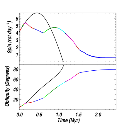
Figure 4: Spin (top) and obliquity (bottom) evolutions in simulation 7. Black lines show the rigid-body evolution. Colored lines show the actual evolution of the aggregate; each color represents a new shape with a corresponding torque. The spin evolution is weakly stochastic, resulting in mild YORP self-limitation. The spin reaches 80% of the maximum rigid-body rate and eventually stagnates at a $\sim 14\mbox{$\rm\,h$}$ period. The obliquity changes monotonically and more resembles a YORP cycle, but asymptotes to an unusual end state of $80\arcdeg$.

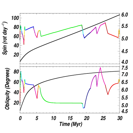
Figure 5: Spin (top) and obliquity (bottom) evolutions in simulation 14, similar to Fig. 4. Black lines and left scales show the rigid-body evolution. Colored lines and right scales show the evolution of the aggregate. Both spin and obliquity evolutions are highly stochastic and result in strong self-limiation.

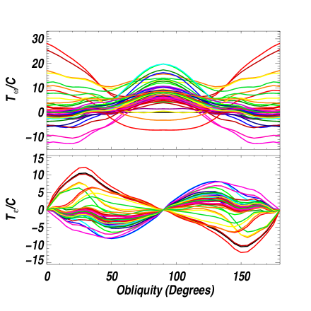
Figure 6: The obliquity (bottom) and the spin (top) torques (YORP curves) through which the aggregate object in simulation 14 (Fig. 5) evolves. The torque components divided by the moment of inertia (in units of $10^{-18}\mbox{$\rm\,s$}^{-2}$) are plotted against the obliquity in degrees. Each colored curve corresponds to a new shape of the aggregate object after a movement of material, and corresponds to the segment of the same color in Fig. 5.

3.1.1 Stochastic YORP

Eleven of the 16 objects exhibit stochastic YORP in their spin evolution, and an equal number (though not exactly the same objects) do so in their obliquities. The upper panel of Fig. 4 shows an example of weak stochasticity in the spin evolution of the object in simulation 7. The evolution has qualitative similarities to the YORP cycle prediction shown in black, and many of the movements of material have only a slight effect on the YORP torques. Nonetheless, the spin evolution changes direction multiple times due to changes in the shape of the object. The obliquity evolution, shown in the lower panel, is monotonic, with greater similarity to a YORP cycle (which we discuss in section 3.1.4 below), demonstrating that different types of YORP behavior can be seen in a single object at the same time.

An example of strongly stochastic YORP is shown in Fig. 5. Here, nearly every change in shape results in a significant change in both components of torque, and often a change in their signs. The scale of these changes can best be seen by looking at the sequence of YORP curves that describe the shapes through which the object evolves. This sequence is shown in Fig. 6; keep in mind that the object evolves along only a small fraction of each pair of YORP curves before shifting to a new pair. As a result of these shifts, strong YORP self-limitation confines spin and obliquity to narrow intervals. Note that one can discern a few longer-lived YORP-cycle-like episodes in Fig. 5 (e.g., between 7 and $18\mbox{$\rm\,Myr$}$); but the time variability is non-repeating and unpredictable.

One can think of stochastic YORP as arising from two coupled effects. First is the shape evolution itself, which causes the object to random-walk among topographic configurations, each producing different YORP torques. Second is the natural tendency for an evolving object to spend more time in configurations that produce smaller torques, simply because it takes longer to build up a sufficient change in spin to trigger a reconfiguration. Hence some points in the topographic space are “stickier” than others, and the time an object may dwell in each configuration is a function of the nearby topographic landscape and its past history. “Sticky” low-torque configurations are also the cause of YORP stagnation, which we discuss below.

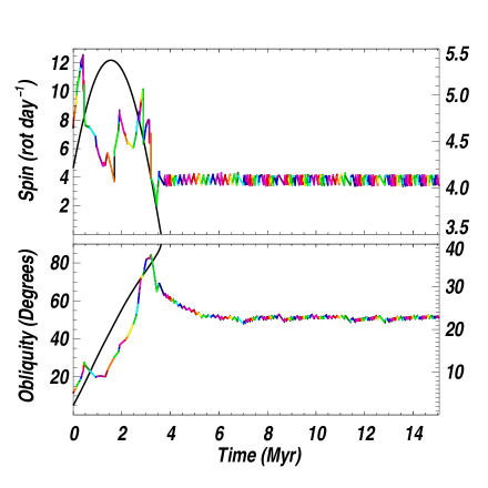
Figure 7: Spin (top) and obliquity (bottom) evolutions in simulation 12. Black lines and left scales show the rigid-body evolution. Colored lines and right scales show the evolution of the aggregate. The evolution is stochastic for the first $3.7\mbox{$\rm\,Myr$}$, after which it becomes self-governed, toggling between neighboring configurations that alternately accelerate and decelerate the spin.

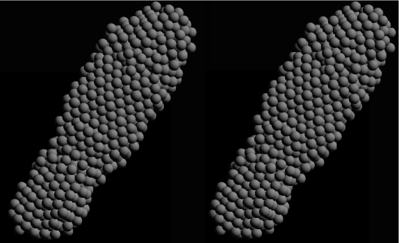
Figure 8: The two configurations between which the object in simulation 12 toggles in the self-governed phase of its evolution (Fig. 7). The view is along the rotation axis. Notice that the object bends at the constriction, one third of the way up from the bottom.

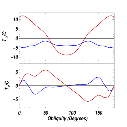
Figure 9: Components of torque (YORP curves) generating changes in (top) spin and (bottom) obliquity for the two toggling configurations in simulation 12 (Fig. 8).

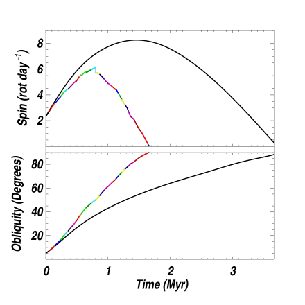
Figure 10: Spin (top) and obliquity (bottom) evolutions in simulation 5, as in Fig. 4. Only one change in the sign of the spin component of torque occurs, resulting in evolution that resembles a modified YORP cycle.

3.1.2 Self-Governed YORP

Three objects show self-governing behavior in their spins, and two of these are also self-governed in obliquity (the third having already evolved to an $\epsilon=0$ orientation before self-governing begins). Figure 7 shows simulation 12, which evolves stochastically in spin and obliquity for the first $3.7\mbox{$\rm\,Myr$}$, but then abruptly begins toggling between two neighboring configurations, one generating a positive, and the other a negative, component of YORP torque along the spin axis. The resulting increases and decreases in spin rate trigger alternating movements of material that convert one configuration into the other. We invariably see self-governing YORP resulting in strong self-limitation of spin and obliquity between narrow limits.

Owing to the unavoidable low-amplitude bouncing of spheres in the HSDEM algorithm, successive appearances of the two configurations are not quite identical, and so the toggling is not quite periodic. In some cases we see self-governing come to an end and return to stochastic evolution, possibly due to this non-repeatability. We can conjecture that a different computational approach that allows the particles to come to rest with respect to each other might show truly periodic switching that continues indefinitely.

Examples of the positive- and negative-torque configurations from simulation 12 are shown in Fig. 8, and the torques that they generate as functions of obliquity are shown in Fig. 9. At obliquity values between 20 and 30 degrees, where the toggling occurs, one configuration has positive values of the spin and obliquity torques while the other one has negative values. A subtle bending at the constriction, one third of the way up from the bottom, results in a change in sign of the obliquity and the spin torques. Note that, as a result of the centrifugal kneading, parts of the object have settled into ordered packing, giving it a “head-tail” structure composed of two more rigid (packed) chunks joined by a flexible waist. This suggests the possibility that known “head-tail” or contact binary objects might also be found in self-governing states.

3.1.3 Stagnating YORP

A close look at Fig. 4 shows that the object in simulation 7 does not reach, or even approach, the expected YORP-cycle end state of $90\arcdeg$ obliquity and zero spin, but instead asymptotes to a moderately slow spin rate ($\sim 2$ day period) at an obliquity of $80\arcdeg$. This is an example of stagnating YORP, which we see in 4 of the 16 objects simulated at the standard TACO resolution and in 2 of the 4 objects re-run at higher resolution. Technically, stagnation is just a special case of stochasticity, in which, as a result of multiple mass movements, an object randomly falls into a configuration of very low torque. What makes it distinct from stochastic YORP is that objects can remain “stuck” in such configurations for times that approach expected NEA lifetimes, effectively shutting off their YORP evolution.

3.1.4 Modified YORP Cycle

Not every object is equally susceptible to small changes in topography, and not every shape reconfiguration necessarily reverses the direction of spin or obliquity evolution. For roughly one-third of our test objects, shape changes affect only the rate of evolution, and as a result these objects follow what we refer to as a modified YORP Cycle. Figure 10 shows simulation 5 as an example. This object approaches the same end state as its rigid counterpart, in a shorter elapsed time, having accelerated to, and decelerated from, a lower maximum spin rate. Another example is seen in the obliquity evolution of simulation 7 (Fig. 4, lower panel), which is monotonic and resembles the rigid-body prediction until it stagnates. Table 2 shows that the duration of the modified YORP cycle can be either longer or shorter than the rigid-body cycle.

Rozitis and Green (2013) and Kaasalainen and Nortunen (2013) have argued that greater topographic sensitivity is a characteristic of objects with weaker overall YORP torques, suggesting that objects that are more instrinsically “yorpy” might be more likely to follow a modified YORP cycle. However, we see no tendency for self-limited or modified YORP cycle behavior to be correlated with the magnitudes of either the initial torques on the test objects or the episodic torques during the aggregate evolution.

3.1.5 End States

The fifth column of Table 2 and the third column of Table 3 give the YORP cycle end-state spins and obliquities, for objects evolving as rigid bodies. The ninth and fourth columns (respectively) of those tables give the corresponding quantities for the aggregate objects at the ends of the simulations.

Two of the 16 objects have rigid-body end states of formally infinite spin; the remaining 14 have rigid-body end state spins of zero, reached in finite time $t_{\rm YC}$. As we have emphasized, most aggregates do not reach or approach the rigid-body end states: only 5 aggregates have spun down to zero or are monotonically decelerating at slow spin rates at the end of the simulations. One object has fissioned, but the majority have either stagnated (2) or are stochastically wandering (8) at finite spin rates, at simulation end times averaging $2.5t_{\rm YC}$. The situation is similar for obliquity. All 16 objects have rigid-body obliquity end states at, or nearly at, $90\arcdeg$. Among the aggregates, roughly half (7) have reached this obliquity or are clearly on their way there as of the end of the simulation. Of the 8 remaining objects that do not fission, 3 have reached different constant values of obliquity, and 5 are wandering stochastically.

Two of the four simulations with higher resolution tilings have rigid-body end states of formally infinite spin and the other two have rigid-body end state spins of zero, reached in finite $t_{\rm YC}$ while the four aggregate objects wander up and down in spin stochastically. In the case of obliquity, the rigid bodies have end states at obliquity values between $73\arcdeg$ and $86\arcdeg$ while the aggregates are stochastically wandering. Three of the four aggregates stagnate at certain values as well, two of them at nearly $0\arcdeg$.

The clear tendency for a majority of aggregates not to evolve to the standard YORP-cycle end states has important implications for orbital evolution due to the Yarkovsky effect. We return to these issues in section 4 below.

3.2 Mass Movement

An important aspect of the mass motion events is that the moving material is not restricted to the surface of the object. Animations of the shape evolution clearly show the entire object reconfiguring (albeit often subtly) rather than material migrating along the surface. To quantify the amount of deep motion in each event, we sort the pkdgrav spheres in order of effective potential $\Phi_{\rm eff}=\Phi-{1\over 2}\omega^{2}R^{2}$, where $\Phi$ is the gravitational potential, $\omega$ is the rotational angular frequency, and $R$ is the cylindrical radius from the spin axis. Each sphere is given an enclosed-mass-fraction coordinate equal to its position in the sorted list divided by the number of spheres. We then tally the number of times that the sphere at each mass fraction coordinate moves by more than $25\%$ of its radius during the simulation.

Figure 11 shows the cumulative distributions of the movements as functions of the mass fraction for all of the simulations. Though the outer layers are somewhat more mobile, there is clearly motion of material all the way into the deep interior. Between 25% and 40% of the mass motion events occur in the inner (i.e., most tightly bound) half of the mass. The outer 10% of the mass accounts for only 15% to 25% of the motion. The freedom to reconfigure internally is what gives the objects the ability to acquire greater rigidity with time, in these simulations by falling into ordered packing. The figure also shows that objects that shed mass (solid curves) tend to exhibit more deep motion than those that do not (dashed curves). We will see below that this is likely related to large-scale shape changes that promote mass shedding.

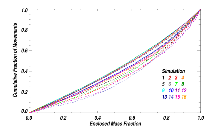
Figure 11: Normalized cumulative distribution of mass-movement events for the 16 simulations as a function of enclosed (by surfaces of constant effective potential) mass fraction. Each color corresponds to a different simulation. Solid lines indicate the 5 objects that exhibit mass-loss episodes.

3.3 Mass Loss and Binary Formation

Five of the 16 simulations experience mass-loss episodes. The first 4 columns of Table 4 show the number of mass-loss events, the total percentage of mass lost from the initial object, and the average time between events for the 5 simulations. Figure 12 shows the distribution of events in terms of the mass lost per event and the rotation period at the time of the event. The minimum mass loss in a single event is $0.1\%$ (one sphere) while the maximum is $2.0\%$. The mass-loss episodes can occur as isolated events or as a chain of events. The average time between events can be as short as $0.01\mbox{$\rm\,Myr$}$ for consecutive events and more than $1\mbox{$\rm\,Myr$}$ for isolated events.

Table 4: Mass-Loss Events

Simulation	$N_{\rm ev}$a	$\Delta M$(%)b	$\langle\Delta t\rangle$c	$\left\langle\rho\right\rangle$d	$P_{\rm min,sph}$e	$\langle\left({b\over a}\right)_{\rm ev}\rangle$f	$P_{\rm min,pro}$g	$\langle P_{\rm ev}\rangle$h
4	10	7.0	0.05	1.42	2.77	0.76	3.18	4.22
8	10	6.1	0.01	1.53	2.67	0.52	3.72	4.49
10	13	6.3	0.15	1.46	2.73	0.91	2.86	4.19
11	18	7.6	1.71	1.48	2.71	0.58	3.57	4.53
15	13	5.1	0.04	1.57	2.63	0.71	3.12	4.08

^a Number of events. ^b Total mass lost (percent). ^c Mean time between events (Myr). ^d Mean bulk density at time of mass loss ($\mbox{$\rm\,g$}\mbox{$\rm\,cm$}^{-3}$). ^e Minimum spin period (h) for cohesionless sphere of the same density. ^f Mean axis ratio at time of mass loss. ^g Minimum spin period (h) for cohesionless prolate spheroid of the same density and axis ratio. ^h Mean spin period (h) at time of mass loss.

Figure 12: The distribution of all mass-loss events. The fraction of the initial body mass that is lost is plotted against the spin period at the time of mass loss. A single sphere corresponds to $0.1\%$ of the initial mass. Mass loss occurs at a mean rotation period of 4.3 hours.

The rotation periods at which mass loss occurs range from 3.8 to 4.6 hours, with a mean of 4.3 hours. The averages for each simulation are listed in the last column of Table 4. These spin rates are substantially slower than the nominal spin limits at which loose material should become unbound from the equator of a sphere with the same bulk density. The fifth and sixth columns of Table 4 give the densities for each simulation, averaged over mass-loss events, and the corresponding limiting periods for spheres. The latter are between 2 and 3 hours. Part of the difference can be attributed to the fact that in our simulations mass is commonly lost from one end of the object as its shape becomes elongated (an example, just before the event, is shown in Fig. 13). The axis ratios $b/a$ in the plane normal to the spin axis, again averaged over events for each simulation, are given in column 7 of Table 4, and column 8 gives the limiting spin period for prolate spheroids of the same axis ratio and density (Harris 1996, Richardson et al. 2005). The theoretical limits are still 20% to 30% slower than the simulation results. We can speculate that this difference may be caused by the tendency for our objects to become sharply pointed at the ends, by non-uniformity of the interior bulk density, or by the dynamical motion of the material close to the tip.

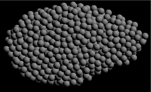
Figure 13: The shape of the aggregate object in simulation 11 before having its first mass-loss episode, in which it loses 3 spheres. The view is along the rotation axis. Material is lost from the right side.

The spheres are removed from the simulations after being shed from the main object. We do not track their orbital evolution since the main objects become strongly prolate. Scheeres (2007) has shown that objects orbiting a rapidly rotating prolate body would most likely escape rather than reach stable orbits where they could accrete to form a binary companion. However, we do encounter one case of binary formation. Figure 14 shows the spin and obliquity evolutions of the object in simulation 8. Black squares indicate mass loss episodes. After losing $6.1\%$ of its initial mass in 9 events, the objects splits in two (at a time of about 2.5 Myr, at which point the simulation is stopped). At the moment of fission, the object is increasing in angular momentum but decreasing in spin rate because of its evolution toward an elongated shape. Figure 15 shows the aggregate at the last point of contact. Note the wasp-waist constriction, where the fission occurs. After fission, the primary object contains $52.7\%$ of the initial mass while the secondary contains $41.2\%$.

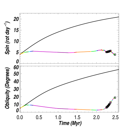
Figure 14: The spin (top) and obliquity (bottom) evolutions of the object in simulation 8, as in Fig. 4. Black and colored lines show the rigid-body evolution and aggregate evolution, respectively. Black squares indicate mass-loss episodes. At the end of the simulation the object fissions to form a binary.

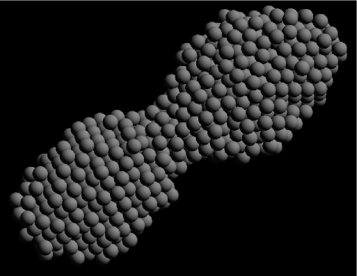
Figure 15: The shape of the aggregate in simulation 8 at the last point of contact before splitting and forming a binary asteroid. The view is along the rotation axis.

3.4 Axis-Ratio Evolution

Figure 16 shows the evolution of the 16 objects in the space of triaxiality $T$ and semi-axis ratio $c/a$, where $T$ is given by equation 4. Each simulation is shown in a different color. Squares indicate the initial objects, as in Fig. 3; each object at the end of the simulation is indicated by an X. Solid curves identify the 5 objects that lose mass. Most objects are still evolving in spin at the end of the simulation and therefore the X does not necessarily represent an evolutionary end point.

The majority of objects (13 of 16) become flatter ($c/a$ decreases) during the simulation. Evolution in triaxiality can go in either direction, but we note two striking trends. First, all objects following a modified YORP cycle (simulations 1, 2, 3, 5, and 16) evolve toward smaller $T$; that is, they become less prolate and more oblate. This appears to be a result of the deceleration to very slow spin rates, although it is important to note that the evolution does not follow a fluid sequence, which would imply $T\to 0$ at finite $\omega$. These objects arrive at genuine non-rotating end states with non-zero $T$. Second, all of the objects that shed mass or fission (simulations 4, 8, 10, 11, and 15) evolve toward smaller $c/a$ and larger $T$; that is, they become highly elongated and prolate. Moreover, these 5 simulations show the largest changes in axis ratio. We conjecture that these objects were the most initially deformable, which is consistent with the finding (Fig. 11) that they also show the greatest amount of deep mass motion. The smooth black line in Fig. 16 indicates the sequence of Jacobi ellipsoids. The objects that lose mass are the only objects that dip well below the Jacobi sequence, and the episodes of mass loss from the endpoints (small diamonds) occur exclusively below the sequence, as does the final fissioning of simulation 8.

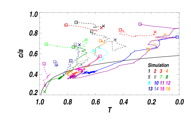
Figure 16: Shape evolution of simulated aggregates, in terms of triaxiality $T$ and semi-axis ratio $c/a$, as in Fig. 3. Each color corresponds to a different simulation. Squares and crosses indicate shapes at the start and end of each simulation, respectively. The 5 simulations that shed mass are plotted with solid lines; mass-loss epsiodes are marked with small diamonds. The smooth black curve indicates the sequence of Jacobi ellipsoids.

3.5 The Statistical Spin and Obliquity Evolutions

Stochastic processes, while non-deterministic, can still be described statistically. Here we formulate a statistical description of the spin-state evolution obtained from our simulations, intended to inform models of spin-dependent processes, particularly the Yarkovsky effect. This description should be regarded as very preliminary: first, because our initial conditions were chosen to survey a variety of interesting YORP behaviors, and not to represent a realistic population of objects; and second, because at this point we are still neglecting processes known to be important, such as thermal conduction.

We break the evolution into discrete intervals bounded by material movements (shape changes). The shape is constant (except for small bouncing of the spheres) during each interval. Consider one such interval of duration $\delta t$, over which the change in spin rate is $\delta\omega$. We define the statistical spin evolution, $\alpha_{s}$, by

$$\alpha_{s}=\pm\left|{\delta\omega}\over{\delta t}\right|,$$ (5)

where the sign is determined by whether the sign of $\delta\omega$ is the same as ($+$) or opposite to ($-$) that in the previous interval. With this definition, rapidly alternating spin-up and spin-down behavior, characteristic of self-governed YORP, would be described by consistently negative values of $\alpha_{s}$. Strongly stochastic YORP would produce a tendency for negative $\alpha_{s}$, while weak stochasticity or modified YORP cycle evolution would appear as predominantly positive values.

Similarly, we define the statistical obliquity evolution, $\zeta_{s}$, in terms of the change of obliquity during the interval according to

$$\zeta_{s}=\pm\left|{\delta\epsilon}\over{\delta t}\right|,$$ (6)

with the sign determined by comparison with the previous interval, as above.

Figure 17 shows the joint distribution in $(\alpha_{s},\delta t)$ and $(\zeta_{s},\delta t)$ for all intervals in all simulations. One can see that typically a few $10^{4}\mbox{$\rm\,yr$}$ elapses between shape changes, and significant alterations to the spin evolution can generally be expected on $\sim 10^{5}\mbox{$\rm\,yr$}$ time scales, for the km-sized objects considered here. The shapes of the distributions in $\alpha_{s}$ and $\zeta_{s}$ are actually surprisingly similar, showing a slight overall tendency toward weak stochasticity. Similar $(\alpha_{s},\zeta_{s},\delta t)$ distributions derived from unbiased initial conditions, with all relevant input physics, will provide a pathway for stochastic YORP to be included, in a Monte Carlo sense, in simulations of orbit evolution that incude the Yarkovsky effect.

Figure 17: Scatter plots of the distribution of (top) $(\alpha_{s},\delta t)$, and (bottom) $(\zeta_{s},\delta t)$, defined in Eqs. (5) and (6). The horizontal axis is the base-10 logarithm of the time interval $\delta t$ in Myr.

4 Discussion

The simulations presented here strongly support the conjecture of Statler (2009) that YORP can behave stochastically when the surface topography is susceptible to spin-driven alterations. We actually see four distinct types of behavior, three of which—stochastic YORP, self-governed YORP, and stagnating YORP—collectively give rise to the phenomenon of YORP self-limitation.

It is a widely held view that YORP is responsible for the formation of top-shaped asteroids, and particularly top-shaped asteroids with binary companions. This view has been shaped, in large part, by the influential simulations of Walsh et al. (2008). By continually adding angular momentum, ostensibly supplied by YORP, the authors were able to make idealized aggregates evolve, through motion of surface material, to nearly axisymmetric top shapes with equatorial ridges, which then shed mass that accreted in orbit to form binaries. But as we have demonstrated in this paper, YORP should not be presumed to be an inexhaustable source of angular momentum. Self-limitation is likely to intervene, possibly stalling the mechanism before substantial evolution has a chance to occur.

In a follow-up study, Walsh et al. (2012) show that the distinctive evolutionary path taken by their earlier aggregates was in part a consequence of the rigidity resulting from the initial HCP arrangement of identical spheres. Altering the size distribution or the initial arrangement to avoid HCP makes the aggregates more fluid, and tends to inhibit both evolution to axisymmetry and mass shedding. Our test objects, while composed of identical spheres, start with a disordered packing. Except for those that follow a modified YORP cycle, our objects generally evolve toward more elongated shapes. The minority that do lose mass do so mostly in modest amounts from their elongated tips; we see only one case of fission into two comparably sized bodies. In these respects their behavior falls between the “near-fluid” and “intermediate” cases of Walsh et al. (2012). Owing to the strongly time-varying potential, we would not expect the slowly-shed mass to accumulate on stable orbits, and consequently not form long-lived binaries.

Exactly how YORP self-limitation may occur on objects with less deformable interiors is a question that we cannot fully address with the present set of simulations. We do observe parts of our aggregates, through time-varying centrifugal massaging, occasionally falling into a HCP state. This tends to happen after some amount of reshaping has already occurred, leading to localized off-center chunks of higher rigidity rather than a central rigid core. We would not expect real objects to “crystallize” in this way, but a real aggregate may naturally develop rigidity as a result of time varying stresses that allow its components to find interlocking configurations. This is a question for future simulations that can take more physical effects into account with greater realism (see below).

In approximately two-thirds of the cases we have simulated, YORP self-limitation prevents objects from decelerating to zero spin rate. These objects never complete a YORP cycle; consequently one would expect them to avoid a chaotic tumbling phase, and hence to preserve their original sense of spin (direct or retrograde). This has bearing on the fraction of retrograde rotators among the NEAs. Studies of the delivery of NEAs from the Main Belt (Bottke et al. 2002, La Spina et al. 2004) conclude that approximately $37\%$ should arrive as a result of inward Yarkovsky drift, requiring retrograde rotation, into the $\nu_{6}$ secular resonance. The rest should come through other resonances with an equal fraction of retrograde and direct rotators. We should therefore expect about $69\%$ of NEAs to have been delivered to their current orbits with retrograde rotation. But from measurements of Yarkovsky drift in the present NEA population, Farnocchia et al. (2013) estimate the retrograde fraction to be just that, i.e., $69\%$, implying that few of the objects have forgotten their original spin sense. Self-limitation may possibly account for this. If we assume that all NEAs with Yarkovsky drift measurements are aggregates, then about $25\%$ out of the $37\%$ of NEAs delivered through $\nu_{6}$ will be prevented from forgetting their initial senses of spin. Adding half of the $12\%$ of the $\nu_{6}$ objects that do forget, plus half of the $63\%$ that come through other resonances, we should expect roughly $63\%$ retrograde rotators, not inconsistent with the observational result. While the statistical uncertainties are substantial, and our simulations are not yet definitive, YORP self-limitation may provide a means to reconcile the high present-day retrograde fraction with the long lifetimes of NEAs relative to their nominal YORP-cycle timescales.

The tendency for self-limited, and particularly stochastic, YORP to preserve a memory of earlier spin states is also relevant to the spreading of collisional families by the Yarkovsky effect. Bottke et al. (2013) find that the envelopes, in $(a,H)$ space, of old families (ages $\sim 1\mbox{$\rm\,Gyr$}$) are inadequately fit by models in which the spin sense of objects is frequently reset, as would happen at the end of a YORP cycle. Instead, a stochastic YORP model, in which the memory of the spin state, and hence the direction of Yarkovsky drift, is preserved for longer times, results in a much better fit. These results are encouraging for the general picture of stochastic YORP, and furthermore hint that even relatively small collisional fragments in the Main Belt may be re-accreted aggregates. We can anticipate that a statistical description, as in Fig. 17, of future results of a more exhaustive, unbiased suite of simulations will help to clarify the situation further.

In the interest of computational expediency, we have neglected physical effects that are known to be important to YORP, and therefore the simulations presented here should be interpreted as a first demonstration of processes that may occur, and not (yet) a definitive depiction of what does occur. The key effects to be explored in future simulations should include:

• Thermal conduction: At a given orientation, this has no direct impact on the spin component of torque, but does affect the obliquity component. Since all components are obliquity-dependent, the coupled evolution will change. One indicator of this dependence is that the rigid-body, YORP-cycle obliquity end states are expected to be concentrated near $0\arcdeg$ for direct rotators with moderate thermal inertia $\Gamma$ (Čapek and Vokrouhlický 2004), rather than $90\arcdeg$ when $\Gamma=0$ (see Table 3). As a check, we have computed the torques on our initial objects, taking into account thermal conduction as well as self-heating (see below), with an assumed $\Gamma=200\mbox{$\rm\,J\,m^{-1}\,s^{-1/2}\,K^{-1}$}$, and verified that the rigid body end states do, in fact, shift to $0\arcdeg$.

• Self-heating: Where concavities exist, parts of the surface can be heated by light reflected or radiated from other parts of the surface. This effect tends to reduce local temperature gradients caused by self-shadowing, which Rozitis and Green (2013) argue may somewhat lessen the sensitivity of YORP to small surface changes. To gauge the potential influence of this effect on our results, we have recalculated the YORP curves for the sequence of objects in simulation 14 (Fig. 6) with a full treatment of self-heating and partial sky blockage. While the torques on individual objects are changed by typically 10% to 50%, the variety and spread of YORP curves in Fig. 6 is qualitatively unaltered. Hence we expect YORP self-limitation and stochasticity still to occur. Rozitis and Green (2013) further suggest that self-heating will act to prevent cases in which the spin component of torque has the same sign at all obliquities. We have “spot-checked” this suggestion on a few objects, including our one initial object that shows a purely positive spin torque. We do find a tendency for these YORP curves to be shifted vertically so that they cross zero. This effect may have bearing on self-governing, which, in our simulations, tends to take advantage of these single-sign configurations (e.g., Fig. 9). However, not all of our self-governing objects rely on such configurations; and furthermore, eliminating the single-sign cases does not preclude the possibility of self-governing at a different obliquity, or of the object finding a different nearby pair of configurations that are self-governing. Settling the issue of whether self-heating prevents self-governing will require calculating the full self-consistent evolution with all relevant thermal effects included.

• Friction and cohesion: The hard-sphere approach to contact physics is only one of several alternatives, and there are indications that it may not be the optimal choice for the dense regime in which particles spend more time in contact than apart (Richardson et al. 2011). One recently developed approach is the soft-sphere discrete element method (SSDEM), newly implemented in pkdgrav by Schwartz et al. (2012). SSDEM permits a more accurate treatment of multicontact physics, including self-consistent treatment of sliding and rolling friction and interparticle cohesion. New numerical experiements on disruptive collisions using SSDEM (Ballouz et al. 2014) are largely in accord with earlier experiments using HSDEM (Leinhardt et al. 2000), so one does not expect results for spin-driven reshaping to differ qualitatively purely because of the computational approach. However in future work we plan to take advantage of the capabilities of SSDEM in order to explore a wider range of material properties, to more realistically account for the effects of irregular particle shapes, and to test strength models for cohesive aggregates (e.g., Schwartz et al. 2013, Sánchez and Scheeres 2014). Recent observational results strongly suggest that cohesive forces are important both in maintaining the integrity of rapidly rotating objects (Rozitis et al. 2014) and in influencing the mode of mass loss (Hirabayashi et al. 2014).

5 Summary

We have presented the first self-consistent simulations of the coupled spin and shape evolutions of small gravitational aggregates under the influence of the YORP effect. Because of the sensitivity of YORP to detailed surface topography, even small centrifugally driven reconfigurations of an aggregate can alter the YORP torque dramatically, resulting in spin evolution that is, in the strong majority of cases, qualitatively different from the rigid-body prediction.

One-third of the objects simulated follow a simple evolution that can be described as a modified YORP cycle. Two-thirds exhibit one or more of three distinct behaviors—stochastic YORP, self-governed YORP, and stagnating YORP—which together result in YORP self-limitation. Self-limitation has the effect of confining the rotation rates of evolving aggregates to far narrower ranges than would be expected in the YORP-cycle picture, and greatly prolonging the times over which objects can preserve their sense of rotation (direct or retrograde).

The simulated asteroids we have tested are initially randomly packed, disordered aggregates of identical spheres that collectively have a low internal angle of friction. They are highly deformable and lie near, but not on the Maclaurin/Jacobi sequence. Their evolution in shape is charaterized by rearrangement of the entire body, including the deep interior, and not predominantly by movement of surface material. Unlike the high-friction-angle initial configurations tested by Walsh et al. (2008), they do not evolve to axisymmetric top shapes with equatorial ridges. When they lose mass, they generally do so in small amounts from the ends of a prolate-triaxial body, and always after crossing the Jacobi ellipsoid sequence.

YORP self-limitation may inhibit the formation of top-shapes, binaries, or both, by restricting the amount of angular momentum that can be imparted to a deformable body. Stochastic YORP, in particular, will affect the evolution of collisional families whose orbits drift apart under the influence of Yarkovsky forces, in observable ways.

The authors are grateful to colleagues for helpful comments during the course of this work, including David Rubincam, Steve Paddack, Steve Chesley, Dan Scheeres, Bill Bottke, David Vokrouhlický, and Mangala Sharma. TSS and DCF were supported in part by NASA Planetary Geology & Geophysics grant NNX11AP15G. TSS was also supported by the Independent Research and Development program while on detail to NSF under the Intergovernmental Personnel Act; the results and opinions expressed in this paper are those of the authors and do not reflect the views of the National Science Foundation. DCF received additional support from a NASA Harriet G. Jenkins Predoctoral Fellowship and a NASA Ohio Space Grant Consortium Doctoral Fellowship. DCR acknowledges support from NASA Planetary Geology & Geophysics grant NNX08AM39G and National Science Foundation grant AST1009579. PT acknowledges the support of the Programme Nationale de Planetologie, France. This work has made use of NASA’s Astrophysics Data System Bibliographic Services.

Appendix A Details of the Inter-Code Orchestration

Figures 18 and 19 show a flowchart of the full simulation procedure. Orchestration is handled by a python script, which runs and transfers data between the routines of TACO that compute YORP torques (blue), those of pkdgrav that integrate the particle dynamics (orange), and the additional routines that evolve the spin and obliquity with time (yellow), transform the object in orientation (purple) and tile the object (green).

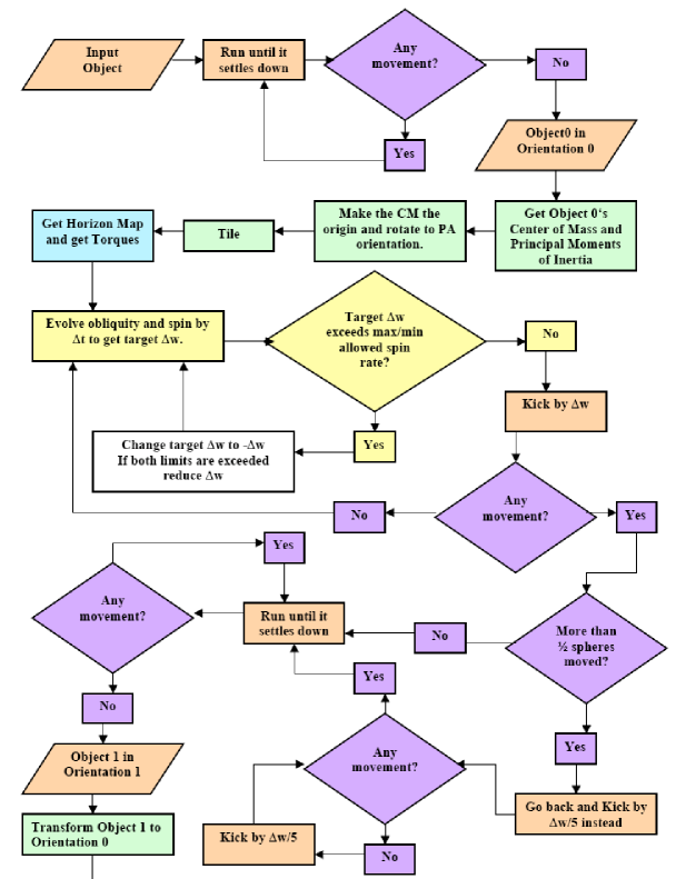
Figure 18: Orchestration flowchart; colors indicate major code elements: TACO (blue), pkdgrav (orange), Spin State Evolution (yellow), Transformation (purple) and Tiling (green).

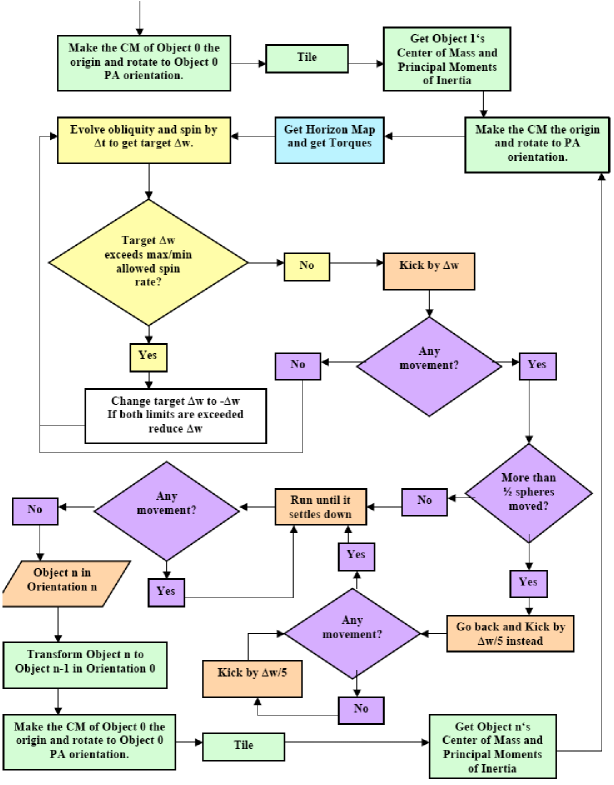
Figure 19: Orchestration flowchart, continued.

We start by dynamically evolving the original object for several rotations at the initial spin rate using pkdgrav. Then we obtain the tiling for the original object (Object 0) with its center of mass as the origin and in principal axis orientation. The YORP torques for the Object 0 are then obtained and we evolve the obliquity and spin in time until the spin rate changes by $0.5\%$ or reaches an extremum. The object is run dynamically with pkdgrav at the new spin rate for several rotations; if there is a movement of spheres we let it evolve for several more rotations until there are no more movements. If, at any movement of material, more than half of the spheres move, we take that as an indication that our increment in spin rate may have been too large. In that case we go back and increment the spin in time instead by $1/5$ of the previous increment until a movement occurs. Once the object has settled down, it is defined as Object 1. We transform it to the orientation of Object 0 in order to obtain the tiling; this guarantees that the tiling is altered only over the regions where motion occurred. Once the tiling is obtained, Object 1 is transformed to its principal axis orientation with its center of mass as the origin and the YORP torques are obtained. The obliquity and spin are evolved in time using the torques of Object 1 until the spin rate changes by $0.5\%$ or reaches an extremum. The object is run dynamically with pkdgrav at the new spin rate for several rotations until there is another movement and a new object is defined, repeating the whole process for each new object (Object n) as was done with Object 1.

References

- Abe et al. (2006) Abe, S., Mukai, T., Hirata, N., Barnouin-Jha, O. S., Cheng, A. F., Demura, H., Gaskell, R. W., Hashimoto, T., Hiraoka, K., Honda, T., Kubota, T., Matsuoka, M., Mizuno, T., Nakamura, R., Scheeres, D. J., Yoshikawa, M., 2006. Mass and Local Topography Measurements of Itokawa by Hayabusa. Science 312, 1344–1349.
- Ballouz et al. (2014) Ballouz, R.-L., Richardson, D. C., Michel, P., Schwartz, S. R., 2014. Rotation-dependent Catastrophic Disruption of Gravitational Aggregates. ApJ789, 158 (12pp).
- Bottke et al. (2013) Bottke, W., Vokrouhlicky, D., Nesvorny, D., Walsh, K., Delbo, M., Lauretta, D., Connolly, H., OSIRIS-REx Team, 2013. The Unusual Evolution of Billion-Year Old Asteroid Families by the Yarkovsky and YORP Effects. In: AAS/Division for Planetary Sciences Meeting Abstracts. Vol. 45 of AAS/Division for Planetary Sciences Meeting Abstracts. p. #106.06.
- Bottke et al. (2002) Bottke, W. F., Morbidelli, A., Jedicke, R., Petit, J., Levison, H. F., Michel, P., Metcalfe, T. S., 2002. Debiased Orbital and Absolute Magnitude Distribution of the Near-Earth Objects. Icarus 156, 399–433.
- Bottke et al. (2006) Bottke, Jr., W. F., Vokrouhlický, D., Rubincam, D. P., Nesvorný, D., 2006. The Yarkovsky and Yorp Effects: Implications for Asteroid Dynamics. Annual Review of Earth and Planetary Sciences 34, 157–191.
- Čapek and Vokrouhlický (2004) Čapek, D., Vokrouhlický, D., 2004. The YORP effect with finite thermal conductivity. Icarus172, 526–536.
- Chesley et al. (2008) Chesley, S. R., Vokrouhlický, D., Bottke, W. F., 2008. Distribution of NEA Spin Axis Obliquities from Measured Thermal Accelerations. In: Bulletin of the American Astronomical Society. Vol. 40 of Bulletin of the American Astronomical Society. p. 435.
- Davis et al. (1979) Davis, D. R., Chapman, C. R., Greenberg, R., Weidenschilling, S. J., Harris, A. W., 1979. Collisional evolution of asteroids - Populations, rotations, and velocities. In: Gehrels, T. (Ed.), Asteroids. University of Arizona Press, pp. 528–557.
- Durech et al. (2008a) Durech, J., Vokrouhlický, D., Kaasalainen, M., Higgins, D., Krugly, Y. N., Gaftonyuk, N. M., Shevchenko, V. G., Chiorny, V. G., Hamanowa, H., Hamanowa, H., Reddy, V., Dyvig, R. R., 2008a. Detection of the YORP effect in asteroid (1620) Geographos. A&A489, L25–L28.
- Durech et al. (2008b) Durech, J., Vokrouhlický, D., Kaasalainen, M., Weissman, P., Lowry, S. C., Beshore, E., Higgins, D., Krugly, Y. N., Shevchenko, V. G., Gaftonyuk, N. M., Choi, Y.-J., Kowalski, R. A., Larson, S., Warner, B. D., Marshalkina, A. L., Ibrahimov, M. A., Molotov, I. E., Michałowski, T., Kitazato, K., 2008b. New photometric observations of asteroids (1862) Apollo and (25143) Itokawa - an analysis of YORP effect. A&A488, 345–350.
- Ďurech et al. (2012) Ďurech, J., Vokrouhlický, D., Baransky, A. R., Breiter, S., Burkhonov, O. A., Cooney, W., Fuller, V., Gaftonyuk, N. M., Gross, J., Inasaridze, R. Y., Kaasalainen, M., Krugly, Y. N., Kvaratshelia, O. I., Litvinenko, E. A., Macomber, B., Marchis, F., Molotov, I. E., Oey, J., Polishook, D., Pollock, J., Pravec, P., Sárneczky, K., Shevchenko, V. G., Slyusarev, I., Stephens, R., Szabó, G., Terrell, D., Vachier, F., Vanderplate, Z., Viikinkoski, M., Warner, B. D., 2012. Analysis of the rotation period of asteroids (1865) Cerberus, (2100) Ra-Shalom, and (3103) Eger - search for the YORP effect. A&A547, A10.
- Farnocchia et al. (2013) Farnocchia, D., Chesley, S. R., Vokrouhlický, D., Milani, A., Spoto, F., Bottke, W. F., 2013. Near Earth Asteroids with measurable Yarkovsky effect. Icarus224, 1–13.
- Gladman et al. (1997) Gladman, B. J., Migliorini, F., Morbidelli, A., Zappala, V., Michel, P., Cellino, A., Froeschle, C., Levison, H. F., Bailey, M., Duncan, M., 1997. Dynamical lifetimes of objects injected into asteroid belt resonances. Science 277, 197–201.
- Hapke (2002) Hapke, B., 2002. Bidirectional Reflectance Spectroscopy 5. The Coherent Backscatter Opposition Effect and Anisotropic Scattering. Icarus 157, 523–534.
- Harris (1996) Harris, A. W., 1996. The Rotation Rates of Very Small Asteroids: Evidence for ’Rubble Pile’ Structure. In: Lunar and Planetary Institute Science Conference Abstracts. Vol. 27 of Lunar and Planetary Institute Science Conference Abstracts. p. 493.
- Helfenstein and Veverka (1989) Helfenstein, P., Veverka, J., 1989. Physical characterization of asteroid surfaces from photometric analysis. In: R. P. Binzel, T. Gehrels, & M. S. Matthews (Ed.), Asteroids II. pp. 557–593.
- Hirabayashi et al. (2014) Hirabayashi, M., Scheeres, D. J., Sánchez, D. P., Gabriel, T., 2014. Constraints on the Physical Properties of Main Belt Comet P/2013 R3 from its Breakup Event. ApJ789, L12.
- Holsapple (2007) Holsapple, K. A., 2007. Spin limits of Solar System bodies: From the small fast-rotators to 2003 EL61. Icarus187, 500–509.
- Kaasalainen and Nortunen (2013) Kaasalainen, M., Nortunen, H., 2013. Compact YORP formulation and stability analysis. A&A558, A104.
- Kaasalainen et al. (2007) Kaasalainen, M., Ďurech, J., Warner, B. D., Krugly, Y. N., Gaftonyuk, N. M., 2007. Acceleration of the rotation of asteroid 1862 Apollo by radiation torques. Nature446, 420–422.
- Kryszczyńska et al. (2007) Kryszczyńska, A., La Spina, A., Paolicchi, P., Harris, A. W., Breiter, S., Pravec, P., 2007. New findings on asteroid spin-vector distributions. Icarus192, 223–237.
- La Spina et al. (2004) La Spina, A., Paolicchi, P., Kryszczyńska, A., Pravec, P., 2004. Retrograde spins of near-Earth asteroids from the Yarkovsky effect. Nature428, 400–401.
- Leinhardt et al. (2000) Leinhardt, Z. M., Richardson, D. C., Quinn, T., 2000. Direct N-body Simulations of Rubble Pile Collisions. Icarus146, 133–151.
- Lowry et al. (2007) Lowry, S. C., Fitzsimmons, A., Pravec, P., Vokrouhlický, D., Boehnhardt, H., Taylor, P. A., Margot, J.-L., Galád, A., Irwin, M., Irwin, J., Kusnirák, P., 2007. Direct Detection of the Asteroidal YORP Effect. Science 316, 272–.
- Lowry et al. (2014) Lowry, S. C., Weissman, P. R., Duddy, S. R., Rozitis, B., Fitzsimmons, A., Green, S. F., Hicks, M. D., Snodgrass, C., Wolters, S. D., Chesley, S. R., Pittichová, J., van Oers, P., 2014. The internal structure of asteroid (25143) Itokawa as revealed by detection of YORP spin-up. A&A562, A48.
- Moré et al. (1984) Moré, J. J., Sorensen, D. C., Hillstrom, K. E., Garbow, B. S., 1984. The MINPACK Project, in Sources and Development of Mathematical Software. Prentice-Hall, Inc., Upper Saddle River, NJ, USA.
- Nugent et al. (2012) Nugent, C. R., Margot, J. L., Chesley, S. R., Vokrouhlický, D., 2012. Detection of Semimajor Axis Drifts in 54 Near-Earth Asteroids: New Measurements of the Yarkovsky Effect. AJ144, 60.
- Ostro et al. (2006) Ostro, S. J., Margot, J.-L., Benner, L. A. M., Giorgini, J. D., Scheeres, D. J., Fahnestock, E. G., Broschart, S. B., Bellerose, J., Nolan, M. C., Magri, C., Pravec, P., Scheirich, P., Rose, R., Jurgens, R. F., De Jong, E. M., Suzuki, S., 2006. Radar Imaging of Binary Near-Earth Asteroid (66391) 1999 KW4. Science 314, 1276–1280.
- Paddack (1969) Paddack, S. J., 1969. Rotational bursting of small celestial bodies: Effects of radiation pressure. J. Geophys. Res.74, 4379–4381.
- Richardson et al. (2005) Richardson, D. C., Elankumaran, P., Sanderson, R. E., 2005. Numerical experiments with rubble piles: equilibrium shapes and spins. Icarus 173, 349–361.
- Richardson et al. (2009) Richardson, D. C., Michel, P., Walsh, K. J., Flynn, K. W., 2009. Numerical simulations of asteroids modelled as gravitational aggregates with cohesion. Planet. Space Sci.57, 183–192.
- Richardson et al. (2000) Richardson, D. C., Quinn, T., Stadel, J., Lake, G., 2000. Direct Large-Scale N-Body Simulations of Planetesimal Dynamics. Icarus 143, 45–59.
- Richardson et al. (2011) Richardson, D. C., Walsh, K. J., Murdoch, N., Michel, P., 2011. Numerical simulations of granular dynamics: I. Hard-sphere discrete element method and tests. Icarus212, 427–437.
- Rozitis and Green (2013) Rozitis, B., Green, S. F., 2013. The influence of global self-heating on the Yarkovsky and YORP effects. MNRAS433, 603–621.
- Rozitis et al. (2014) Rozitis, B., MacLennan, E., Emery, J. P., 08 2014. Cohesive forces prevent the rotational breakup of rubble-pile asteroid (29075) 1950 da. Nature 512 (7513), 174–176.
- Rubincam (2000) Rubincam, D. P., 2000. Radiative Spin-up and Spin-down of Small Asteroids. Icarus 148, 2–11.
- Rubincam and Bottke (2000) Rubincam, D. P., Bottke, W. F., 2000. The YORP Effect and the Spin of Small Asteroids. In: Lunar and Planetary Institute Science Conference Abstracts. Vol. 31 of Lunar and Planetary Institute Science Conference Abstracts. p. 1399.
- Sánchez and Scheeres (2014) Sánchez, P., Scheeres, D. J., 2014. The strength of regolith and rubble pile asteroids. Meteoritics and Planetary Science 49, 788–811.
- Scheeres (2007) Scheeres, D. J., 2007. Rotational fission of contact binary asteroids. Icarus 189, 370–385.
- Scheeres and Gaskell (2008) Scheeres, D. J., Gaskell, R. W., 2008. Effect of density inhomogeneity on YORP: The case of Itokawa. Icarus 198, 125–129.
- Schwartz et al. (2013) Schwartz, S. R., Michel, P., Richardson, D. C., 2013. Numerically simulating impact disruptions of cohesive glass bead agglomerates using the soft-sphere discrete element method. Icarus226, 67–76.
- Schwartz et al. (2012) Schwartz, S. R., Richardson, D. C., Michel, P., 2012. An implementation of the soft-sphere discrete element method in a high-performance parallel gravity tree-code. Granular Matter 14 (3), 363–380.
- Stadel (2001) Stadel, J. G., 2001. Cosmological N-body simulations and their analysis. Ph.D. thesis, University of Washington.
- Statler (2009) Statler, T. S., 2009. Extreme sensitivity of the YORP effect to small-scale topography. Icarus 202, 502–513.
- Statler et al. (2013) Statler, T. S., Cotto-Figueroa, D., Riethmiller, D. A., Sweeney, K. M., 2013. Size matters: The rotation rates of small near-Earth asteroids. Icarus225, 141–155.
- Statler et al. (2004) Statler, T. S., Emsellem, E., Peletier, R. F., Bacon, R., 2004. Long-lived triaxiality in the dynamically old elliptical galaxy NGC 4365: a limit on chaos and black hole mass. MNRAS353, 1–14.
- Tanga et al. (2009) Tanga, P., Comito, C., Paolicchi, P., Hestroffer, D., Cellino, A., Dell’Oro, A., Richardson, D. C., Walsh, K. J., Delbo, M., 2009. Rubble-Pile Reshaping Reproduces Overall Asteroid Shapes. ApJ706, L197–L202.
- Taylor et al. (2007) Taylor, P. A., Margot, J.-L., Vokrouhlický, D., Scheeres, D. J., Pravec, P., Lowry, S. C., Fitzsimmons, A., Nolan, M. C., Ostro, S. J., Benner, L. A. M., Giorgini, J. D., Magri, C., 2007. Spin Rate of Asteroid (54509) 2000 PH5 Increasing Due to the YORP Effect. Science 316, 274–.
- Walsh et al. (2008) Walsh, K. J., Richardson, D. C., Michel, P., 2008. Rotational breakup as the origin of small binary asteroids. Nature454, 188–191.
- Walsh et al. (2012) Walsh, K. J., Richardson, D. C., Michel, P., 2012. Spin-up of rubble-pile asteroids: Disruption, satellite formation, and equilibrium shapes. Icarus220, 514–529.
- Wilkison et al. (2002) Wilkison, S. L., Robinson, M. S., Thomas, P. C., Veverka, J., McCoy, T. J., Murchie, S. L., Prockter, L. M., Yeomans, D. K., 2002. An Estimate of Eros’s Porosity and Implications for Internal Structure. Icarus155, 94–103.