Coding and Decoding Schemes for MSE and Image Transmission

Abstract

In this work we explore possibilities for coding and decoding tailor-made for mean squared error evaluation of error in contexts such as image transmission. To do so, we introduce a loss function that expresses the overall performance of a coding and decoding scheme for discrete channels and that exchanges the usual goal of minimizing the error probability to that of minimizing the expected loss. In this environment we explore the possibilities of using ordered decoders to create a message-wise unequal error protection (UEP), where the most valuable information is protected by placing in its proximity information words that differ by a small valued error. We give explicit examples, using scale-of-gray images, including small-scale performance analysis and visual simulations for the BSMC.

I Introduction

Information of various nature (pictures, movies, voice, music, text, etc.) is compressed using different methods and algorithms (JPEG, MPEG, FLAC, MP3, PDF, etc.), that takes into account the nature of the information and the different loss in distortion that may be caused by different errors. When it comes to information transmission, information is generally considered as just sequences of bits and the actual type of the information is generally ignored. In this work, we consider instances where we do know something about the semantic value of decoding errors. The main idea is the trade-off between the quantity and importance of decoding errors, as is usually done in distortion theory.

We start by defining a general expected loss function, the valued measure of decoding errors, in Section II. With this broad definition in mind, we establish various existence results showing the importance of encoders and decoders, in Section III.

We give a first heuristic approach for image transmission in Section IV, proposing strategies to address the problem of transmitting images over a (very) noisy channel. For this purpose, we consider the mean squared error (MSE) as the value function of decoding errors, proposing both coding and decoding schemes and considering a (syndrome) decoding algorithm that has the advantage of very low complexity. This heuristic approach is developed for a small dimensional case, and includes performance analyses and visual test performed on the sample in Figure 1.

Figure 1: A family of tamarins at the Rio Negro, Amazon rain forest.

Finally, in Section V, we briefly explore the expected loss function when the error measure of decoding is invariant by translations, a situation where the BER (bit error probability) is a particular case of this.

II Expected Loss Function

In this section we define the expected loss function of a code. We begin by introducing some basic concepts and notation, following [1], [2] and [5].

In this work, we consider a discrete channel with input set $\mathcal{X}$ and output set $\mathcal{Y}$, and we assume that $\mathcal{X}\subseteq\mathcal{Y}$. We assume that both $\mathcal{X}$ and $\mathcal{Y}$ are finite sets. The channel is determined by the matrix $\left(P\left(y|x\right)\right)_{y\in\mathcal{Y},x\in\mathcal{X}}$ of conditional probabilities $P\left(y\text{ is received}|x\text{ is sent}\right)$. In subsequent sections we will consider $\mathcal{X}=\mathcal{Y}=\mathbb{F}_{q}^{n}$, the $n$-dimensional vector space over the finite field $\mathbb{F}_{q}$ with $q$ elements, so we stress that $P\left(y|x\right)$ is considered over the words $x=\left(x_{1},\ldots,x_{n}\right)$ and $y=\left(y_{1},\ldots,y_{n}\right)$. We denote a discrete channel by $P_{\mathcal{X},\mathcal{Y}}$.

We consider an information set $\mathcal{I}{\ }$with $M=\left|\mathcal{I}\right|$ elements. A coding-decoding scheme for $\mathcal{I}$ over $P_{\mathcal{X},\mathcal{Y}}$ is a triple $\left(C,f,a\right)$ consisting of: $(i)$ a code $C\subseteq\mathcal{X}$ having $M$ elements; $(ii)$ a channel encoder $f:\mathcal{I}\rightarrow C$, where $f$ may be any bijective map; and $(iii)$ a channel decoder consisting of a surjective map $a:\mathcal{Y}\rightarrow C$. In such a coding-decoding scheme, a piece of information $\iota\in\mathcal{I}$ is encoded as a codeword $c=f\left(\iota\right)\in C$, and, after $c$ is transmitted, a message $y\in\mathcal{Y}$ is received and decoded as $a\left(y\right)$. Because the encoder $f$ is assumed to be a bijection over $C$, the decoding process is completed by assuming the original information was $f^{-1}\left(a\left(y\right)\right)\in\mathcal{I}$.

Let $D\left(c\right)$ be the decision region of $c$ relative to the decoder $a$:

$$D\left(c\right):=a^{-1}\left(c\right)=\left\{y\in\mathcal{Y}:a\left(y\right)=c\right\}\text{.}$$

The decision regions $D\left(c\right)$ of a decoder $a$ determine a partition of $\mathcal{Y}$. Given a coding-decoding scheme, an error occurs if $c$ is sent and the received codeword lies in some decision region $D\left(c^{\prime}\right)$ with $c^{\prime}\neq c$. The word error probability of $c$ is therefore

$$P_{e}\left(c\right)=1-\sum_{y\in D\left(c\right)}P\left(\left.y\right|c\right)\text{.}$$

Assuming that the probability distribution of $C$ is uniform, that is, each codeword $c$ is transmitted with probability $P\left(c\right)=\frac{1}{M}$ with $M:=\left|C\right|$, the word error probability of $C$ (WEP) is the average

$$P_{e}\left(C\right)=\frac{1}{M}\sum_{c\in C}P_{e}\left(c\right)\text{.}$$

We now let $\mathbb{R}_{+}$ denotes the set of non-negative real numbers and consider the map

$$\nu_{0\text{-}1}:C\times C\rightarrow\mathbb{R}_{+}$$

given by

$$\nu_{0\text{-}1}\left(c,c^{\prime}\right)=\left\{\begin{tabular}[c]{ccc}$0$&if&$c=c^{\prime}$\\ $1$&if&$c\neq c^{\prime}$\end{tabular}\ \right.\text{.}$$

It follows that the word error probability may be expressed as

$$P_{e}\left(C\right)=\frac{1}{M}\sum_{c\in C}\sum_{y\in\mathcal{Y}}\nu_{0\text{-}1}\left(a\left(y\right),c\right)P\left(\left.y\right|c\right)\text{.}$$ (1)

The function $\nu_{0\text{-}1}$ is the indicator function, which detects decoding errors (see [5]) but does not distinguish between different such errors.

In many real-world situations, such as the transmission of digital images, it is reasonable to attribute different values to different errors, and this is what will be done in this work, replacing $\nu_{0\text{-}1}$ by value functions that may assume any (non-negative) real value.

An error value function for a set of information $\mathcal{I}$ is a map $\nu$ that associates to each pair of information a non-negative real number

$$\nu:\mathcal{I}\times\mathcal{I}\rightarrow\mathbb{R}_{+}$$

where $\nu\left(\iota_{1},\iota_{2}\right)$ is the cost of exchanging $\iota_{2}$ by $\iota_{1}$. If $C$ is a code and $f:\mathcal{I}\rightarrow C$ is an encoder, we denote by

$$\nu_{f}:C\times C\rightarrow\mathbb{R}_{+}$$

the error value function induced by the encoder $f$: given $\iota_{1},\iota_{2}\in\mathcal{I}$, we define

$$\nu_{f}\left(f\left(\iota_{1}\right),f\left(\iota_{2}\right)\right):=\nu\left(\iota_{1},\iota_{2}\right).$$

We shall refer to $\nu$ and $\nu_{f}$ as just error value functions. By considering such an error value function, we are interested in evaluating the errors that may occur during the process consisting of coding, transmitting and decoding information.

Given a coding-decoding scheme $\left(C,f,a\right)$ and a error value function $\nu_{f}:C\times C\rightarrow\mathbb{R}_{+}$, let us denote by $\mathbb{E}(C,\left.\nu_{f},a\right|y)$ the posterior expected loss of the induced error value function $\nu_{f}\left(c,a\left(y\right)\right)$, given that $y$ is observed:

$$\mathbb{E}(C,\left.\nu_{f},a\right|y)=\sum_{c\in C}\nu_{f}\left(c,a\left(y\right)\right)P\left(\left.c\right|y\right)\text{.}$$ (2)

We define the overall expected loss of the coding-decoding scheme as the average of the expected loss for all possible $y\in\mathcal{Y}$,

$$\mathbb{E}\left(C,a,\nu_{f}\right)=\sum_{y\in\mathcal{Y}}\mathbb{E}(C,\left.\nu_{f}\left(c,a(y)\right)\right|y)P(y),$$

where $P(y)=\sum_{c\in C}P(c)P\left(\left.c\right|y\right)$ is the probability of receiving $y$. Considering Bayes’ Rule, this expression can be rewritten as

$$\mathbb{E}\left(C,a,\nu_{f}\right)=\sum_{c\in C}\sum_{y\in\mathcal{Y}}\nu_{f}\left(c,a\left(y\right)\right)P\left(\left.y\right|c\right)P(c)$$

and thus

$$\mathbb{E}\left(C,a,\nu_{f}\right)=\sum_{\left(c,c^{\prime}\right)\in C\times C}G_{a}\left(c,c^{\prime}\right)\nu_{f}\left(c,c^{\prime}\right)$$ (3)

where

$$G_{a}\left(c,c^{\prime}\right)=\sum_{y\in a^{-1}\left(c\right)}P\left(\left.c^{\prime}\right|y\right)P\left(y\right)\text{.}$$ (4)

In a general setting, we consider the following data to be given:

• The error value function $\nu$ (determined by the nature of the information);

• The size of the code $C$ (determined by $\left|\mathcal{I}\right|$);

• The rate $\left|\mathcal{I}\right|/\left|\mathcal{Y}\right|=\left|C\right|/\left|\mathcal{Y}\right|$ (determined by cost constraints);

• The channel model $P_{\mathcal{X},\mathcal{Y}}$ (determined by physical conditions).

In such a setting, we say that the triple $\left(C^{\ast},f^{\ast},a^{\ast}\right)$ is a Bayes coding-decoding scheme if

$$\mathbb{E}\left(C^{\ast},a^{\ast},\nu_{f^{\ast}}\right)=\min_{\left(C,a,f\right)}\mathbb{E}\left(C,a,\nu_{f}\right)$$

where the minimum is taken over all encoding-decoding schemes for $\mathcal{I}$ over $P_{\mathcal{X},\mathcal{Y}}$.

As expected, determining a Bayes coding-decoding scheme is a (very) hard problem, so we may consider each of the variables $C$, $f$ and $a$ independently and say that $a^{\ast}$ is a Bayes decoder of the pair $\left(C_{0},f_{0}\right)$ if

$$\mathbb{E}\left(C_{0},a^{\ast},\nu_{f_{0}}\right)=\min_{\left(C_{0},a,f_{0}\right)}\mathbb{E}\left(C_{0},a,\nu_{f_{0}}\right)\text{.}$$

Similarly, we say that $f^{\ast}$ is a Bayes encoder of the pair $\left(C_{0},a_{0}\right)$ if

$$\mathbb{E}\left(C_{0},a_{0},\nu_{f^{\ast}}\right)=\min_{\left(C_{0},a_{0},f\right)}\mathbb{E}\left(C_{0},a_{0},\nu_{f}\right)\text{.}$$

III Relevance of Encoders and Decoders

In this section, we show that, in quite general instances, every encoder and every decoder may be relevant, depending on the error value functions to be considered.

We start by remarking that there are two classes of decoders that may be considered to be “universal,” in the sense that they define a decoding criteria $a:\mathcal{Y}\rightarrow C$ for any code $C$ in $\mathcal{X}$. The first class is the probabilistic criterion determined by the channel, known as a maximal likelihood decoder (ML-decoder): given $y\in\mathcal{Y}$, $a\left(y\right)\in C$ satisfies the inequality

$$P\left(y|a\left(y\right)\right)\geq P\left(y|c\right)\text{ for all }c\in C.$$

The second class of universal decoders, relatives to the discrete channels such that $\mathcal{X}=\mathcal{Y}$, are the so-called nearest neighbor decoders (NN-decoders) determined by a metric $d:\mathcal{X}\times\mathcal{X}\rightarrow\mathbb{R}_{+}$: given $y\in\mathcal{X}$, $a\left(y\right)\in C$ satisfies the inequality

$$d\left(y,a\left(y\right)\right)\leq d\left(y,c\right)\text{ for all }c\in C.$$

We start by proving that, for any linear code and any ML-decoder, there are always error value functions for which it is better to use a different decoder.

From here on in this section, we assume that the prior probability of $C$ is uniform.

Theorem 1

Let $\left(C,f,a\right)$ be a coding-decoding scheme over a reasonable discrete channel $P_{\mathcal{X},\mathcal{Y}}$, that is, $P(x|x)>P(y|x)$ for all $y\neq x$. If $a:\mathcal{Y}\rightarrow C$ is an ML-decoder, then there exists a decoder $b:\mathcal{Y}\rightarrow C$ and error value functions $\nu_{f}$ and $\widetilde{\nu}_{f}$ such that

$$\mathbb{E}\left(C,a,\nu_{f}\right)>\mathbb{E}\left(C,b,\nu_{f}\right)\text{ and }\mathbb{E}\left(C,a,\widetilde{\nu}_{f}\right)<\mathbb{E}\left(C,b,\widetilde{\nu}_{f}\right)\text{.}$$

Proof:

Let $C$ be a code, $a:\mathcal{Y}\rightarrow C$ an ML-decoder and $\nu_{f}:C\times C\rightarrow\mathbb{R}_{+}$ the error value function defined by

$$\nu_{f}\left(c,c^{\prime}\right)=\left\{\begin{array}[c]{ccc}1&\text{ if }&c=c^{\prime}\\ 0&\text{ if }&c\neq c^{\prime}\end{array}\right.\text{.}$$

Note that $\nu_{f}$ does not depend of the encoder $f$ and that it may be expressed as $\nu_{f}\left(c,c^{\prime}\right)=1-\nu_{0\text{-}1}\left(c,c^{\prime}\right)$.

We consider now $c_{1},c_{2}\in C$, with $c_{1}\neq c_{2}$, and define $b:=b_{a,c_{1},c_{2}}:\mathcal{Y}\rightarrow C$ by

$$b\left(y\right)=\left\{\begin{array}[c]{ccc}c_{1}&\text{ if }&y=c_{2}\\ c_{2}&\text{ if }&y=c_{1}\\ a\left(y\right)&\text{ otherwise }&\end{array}\right.\text{.}$$

We are considering two different decoders and, for a given error value function, we wish to look at the difference $\mathbb{E}\left(C,a,\nu_{f}\right)-\mathbb{E}\left(C,b,\nu_{f}\right)$. We define

$$G_{a}\left(c\right):=\sum_{y\in a^{-1}\left(c\right)}P\left(c|y\right)P\left(y\right)\text{ and }G_{b}\left(c\right):=\sum_{y\in b^{-1}\left(c\right)}P\left(c|y\right)P\left(y\right)$$

and thus, considering the error value function $\nu_{f}$, we may express the difference

$$\mathbb{E}\left(C,a,\nu_{f}\right)-\mathbb{E}\left(C,b,\nu_{f}\right)=\sum_{c\in C}G_{a}\left(c\right)-\sum_{c\in C}G_{b}\left(c\right)$$ (5)

because $\nu_{f}\left(c,c^{\prime}\right)=0$ if $c\neq c^{\prime}$ and $\nu_{f}\left(c,c\right)=1$ for all $c\in C$.

Because for $y\neq c_{1},c_{2}$ we have that $a_{1}\left(y\right)=a_{2}\left(y\right)$, the equation (5) reduces to

$$\mathbb{E}\left(C,a,\nu_{f}\right)-\mathbb{E}\left(C,b,\nu_{f}\right)=$$

$$P\left(c_{1}|c_{1}\right)P\left(c_{1}\right)+P\left(c_{2}|c_{2}\right)P\left(c_{2}\right)-P\left(c_{1}|c_{2}\right)P\left(c_{2}\right)-P\left(c_{2}|c_{1}\right)P\left(c_{1}\right)$$

and assuming that the probability distribution of $C$ is uniform, we get

$$\mathbb{E}\left(C,a,\nu_{f}\right)-\mathbb{E}\left(C,b,\nu_{f}\right)=$$

$$\frac{1}{M}\left(P\left(c_{1}|c_{1}\right)+P\left(c_{2}|c_{2}\right)-P\left(c_{2}|c_{1}\right)-P\left(c_{1}|c_{2}\right)\right)\text{.}$$

Because

$$P\left(c_{1}|c_{1}\right)>P\left(c_{1}|c_{2}\right)\text{ and }P\left(c_{2}|c_{2}\right)>P\left(c_{2}|c_{1}\right),$$

it follows that

$$\mathbb{E}\left(C,a,\nu_{f}\right)-\mathbb{E}\left(C,b,\nu_{f}\right)>0\text{.}$$

To obtain the inequality

$$\mathbb{E}\left(C,a,\widetilde{\nu}\right)-\mathbb{E}\left(C,b,\widetilde{\nu}\right)<0\text{,}$$

we can consider $\widetilde{\nu}$ to be $\widetilde{\nu}=\nu_{0\text{-}1}$. Because $a$ is an ML-decoder, we have that

$$\mathbb{E}\left(C,a,\widetilde{\nu}\right)<\mathbb{E}\left(C,b,\widetilde{\nu}\right)\text{.}$$

∎

Corollary 1

Suppose $\mathcal{X}=\mathcal{Y}$ and let $\left(C,f,a\right)$ be an coding-decoding scheme over $\mathcal{X}$ such that $a:\mathcal{X}\rightarrow C$ is an NN-decoder determined by a metric $d$. Then, there exists a discrete channel $P_{\mathcal{X},\mathcal{X}}$, a decoder $b:\mathcal{X}\rightarrow C$ and error value functions $\nu_{f}$ and $\widetilde{\nu}_{f}$ such that

$$\mathbb{E}\left(C,a,\nu_{f}\right)>\mathbb{E}\left(C,b,\nu_{f}\right)\text{ and }\mathbb{E}\left(C,a,\widetilde{\nu}_{f}\right)<\mathbb{E}\left(C,b,\widetilde{\nu}_{f}\right).$$

Proof:

The proof follows from Theorem 1 and from the fact that, given a metric $d:\mathcal{X}\times\mathcal{X}\rightarrow\mathbb{R}_{+}$, there is a discrete channel over $\mathcal{X}$ such that the NN-decoder determined by $d$ and the ML-decoder coincide for any code $C\subseteq\mathcal{X}$ (proof to be found in [14]). ∎

From here on, we assume that $\mathcal{X}=\mathcal{Y}$ and write $P_{\mathcal{X},\mathcal{Y}}=P_{\mathcal{X}}$.

Theorem 2

Let $a_{1}\neq a_{2}$ be two NN-decoders defined on $\mathcal{X}$, determined respectively by the metrics $d_{1}$ and $d_{2}$. Then, there is a code $C\subseteq\mathcal{X}$, encoders $f_{1},f_{2}:\mathcal{I}\rightarrow C$, error value functions $\nu_{1},\nu_{2}:\mathcal{I}\times\mathcal{I}\rightarrow\mathbb{R}_{+}$ and an open family of discrete channels $P_{\mathcal{X}}$ over $\mathcal{X}$ such that

$$\mathbb{E}\left(C,a_{1},\nu_{1}\right)>\mathbb{E}\left(C,a_{2},\nu_{1}\right)\text{ and }\mathbb{E}\left(C,a_{1},\nu_{2}\right)<\mathbb{E}\left(C,a_{2},\nu_{2}\right)\text{.}$$

Proof:

Because we are assuming $a_{1}\neq a_{2}\,$, there is a code $C\subseteq\mathcal{X}$ and $y_{0}\in\mathcal{X}\setminus C$ such that

$$c_{1}:=a_{1}\left(y_{0}\right)\neq a_{2}\left(y_{0}\right):=c_{2}$$

Because we are considering NN-decoders determined by metrics, say $d_{1}$ and $d_{2}$, we have that

$$d_{1}\left(y_{0},c_{1}\right)\leq d_{1}\left(y_{0},c\right)\text{ and }d_{2}\left(y_{0},c_{2}\right)\leq d_{2}\left(y_{0},c\right),$$

for all $c\in C$, and in particular

$$d_{1}\left(y_{0},c_{1}\right)\leq d_{1}\left(y_{0},c_{2}\right)\text{ and }d_{2}\left(y_{0},c_{2}\right)\leq d_{2}\left(y_{0},c_{1}\right),$$

hence we may assume, without loss of generality, that $C=\left\{c_{1},c_{2}\right\}$

and thus our information set $\mathcal{I}=\left\{\iota_{1},\iota_{2}\right\}$ has only two elements. We consider the two possible encoders $f_{1},f_{2}:\mathcal{I\rightarrow C}$ by

$$f_{1}\left(\iota_{1}\right)=c_{1},f_{1}\left(\iota_{2}\right)=c_{2}\text{ and }f_{2}\left(\iota_{1}\right)=c_{2},f_{2}\left(\iota_{2}\right)=c_{1}\text{.}$$

Let us consider the induced error value functions

$$\nu_{1}\left(c,c^{\prime}\right)=\left\{\begin{array}[c]{cc}\delta_{1}&\text{ if }\left(c,c^{\prime}\right)=\left(c_{1},c_{2}\right)\\ 0&\text{ otherwise}\end{array}\right.$$

and

$$\nu_{2}\left(c,c^{\prime}\right)=\left\{\begin{array}[c]{cc}\delta_{2}&\text{ if }\left(c,c^{\prime}\right)=\left(c_{2},c_{1}\right)\\ 0&\text{ otherwise}\end{array}\right.$$

Let us define

$$V_{i}^{j}=\left\{y\in\mathcal{X}:a_{j}\left(y\right)=c_{i}\right\},$$

$i,j\in\left\{1,2\right\}$. With this notation, for $i\neq j$, we have that

$$\mathbb{E}\left(C,a_{j},\nu_{i}\right) =\sum_{y\in\mathcal{X}^{n}}\sum_{c\in C}\nu_{i}\left(c,a_{j}\left(y\right)\right)P\left(y|c\right)$$

$$=\sum_{y\in\mathcal{X}^{n}}\nu_{i}\left(c_{i},a_{j}\left(y\right)\right)P\left(y|c_{i}\right)$$

$$=\sum_{y\in V_{j}^{j}}\delta_{i}\cdot P\left(y|c_{i}\right)$$

and

$$\mathbb{E}\left(C,a_{i},\nu_{i}\right) =\sum_{y\in\mathcal{X}^{n}}\sum_{c\in C}\nu_{i}\left(c,a_{i}\left(y\right)\right)P\left(y|c\right)$$

$$=\sum_{y\in\mathcal{X}^{n}}\nu_{i}\left(c_{i},a_{i}\left(y\right)\right)P\left(y|c_{i}\right)$$

$$=\sum_{y\in V_{j}^{i}}\delta_{i}\cdot P\left(y|c_{i}\right)\text{.}$$

Considering the difference between the expected loss functions we find that

$$\mathbb{E}\left(C,a_{1},\nu_{1}\right)-\mathbb{E}\left(C,a_{2},\nu_{1}\right) =\delta_{1}\left(\sum_{y\in V_{2}^{1}}P\left(y|c_{1}\right)-\sum_{y\in V_{2}^{2}}P\left(y|c_{1}\right)\right)$$ (6)

$$=\delta_{1}\left(\sum_{y\in V_{2}^{1}\backslash V_{2}^{2}}P\left(y|c_{1}\right)-\sum_{y\in V_{2}^{2}\backslash V_{2}^{1}}P\left(y|c_{1}\right)\right)$$ (7)

and, similarly,

$$\mathbb{E}\left(C,a_{1},\nu_{2}\right)-\mathbb{E}\left(C,a_{2},\nu_{2}\right)=\delta_{2}\left(\sum_{y\in V_{1}^{1}\backslash V_{1}^{2}}P\left(y|c_{2}\right)-\sum_{y\in V_{1}^{2}\backslash V_{1}^{1}}P\left(y|c_{2}\right)\right)\text{.}$$ (8)

Considering $i\neq j$, we remark now that

$$V_{j}^{i}\backslash V_{j}^{j} =\left\{y\in\mathcal{X}:a_{i}\left(y\right)=c_{j},a_{j}\left(y\right)\neq c_{j}\right\}$$

$$=\left\{y\in\mathcal{X}:a_{i}\left(y\right)=c_{j},a_{j}\left(y\right)=c_{i}\right\}$$

$$=\left\{y\in\mathcal{X}:a_{i}\left(y\right)\neq c_{i},a_{j}\left(y\right)=c_{i}\right\}=V_{i}^{j}\backslash V_{i}^{i}$$

and

$$V_{i}^{i}\backslash V_{i}^{j} =\left\{y\in\mathcal{X}:a_{i}\left(y\right)=c_{i},a_{j}\left(y\right)\neq c_{i}\right\}$$

$$=\left\{y\in\mathcal{X}:a_{i}\left(y\right)=c_{i},a_{j}\left(y\right)=c_{j}\right\}$$

$$=\left\{y\in\mathcal{X}:a_{i}\left(y\right)\neq c_{j},a_{j}\left(y\right)=c_{j}\right\}=V_{j}^{j}\backslash V_{j}^{i},$$

along equations (7) and (8), can be represented as

$$\mathbb{E}\left(C,a_{1},\nu_{1}\right)-\mathbb{E}\left(C,a_{2},\nu_{1}\right)=\delta_{1}\left(\sum_{y\in V_{2}^{1}\backslash V_{2}^{2}}P\left(y|c_{1}\right)-\sum_{y\in V_{2}^{2}\backslash V_{2}^{1}}P\left(y|c_{1}\right)\right)$$

and

$$\mathbb{E}\left(C,a_{1},\nu_{2}\right)-\mathbb{E}\left(C,a_{2},\nu_{2}\right)=\delta_{2}\left(\sum_{y\in V_{2}^{2}\backslash V_{2}^{1}}P\left(y|c_{2}\right)-\sum_{y\in V_{2}^{1}\backslash V_{2}^{2}}P\left(y|c_{2}\right)\right)\text{.}$$

For simplicity, let us write

$$V_{1}=V_{2}^{1}\backslash V_{2}^{2},V_{2}=V_{2}^{2}\backslash V_{2}^{1}\text{.}$$

Thus, we have that

$$\mathbb{E}\left(C,a_{1},\nu_{1}\right)-\mathbb{E}\left(C,a_{2},\nu_{1}\right)=\delta_{1}\left(\sum_{y\in V_{1}}P\left(y|c_{1}\right)-\sum_{y\in V_{2}}P\left(y|c_{1}\right)\right)$$

and

$$\mathbb{E}\left(C,a_{1},\nu_{2}\right)-\mathbb{E}\left(C,a_{2},\nu_{2}\right)=\delta_{2}\left(\sum_{y\in V_{2}}P\left(y|c_{2}\right)-\sum_{y\in V_{1}}P\left(y|c_{2}\right)\right)\text{.}$$

Now, we note that

$$\mathbb{E}\left(C,a_{1},\nu_{1}\right)-\mathbb{E}\left(C,a_{2},\nu_{1}\right)>0\text{ and }\mathbb{E}\left(C,a_{1},\nu_{2}\right)-\mathbb{E}\left(C,a_{2},\nu_{2}\right)<0$$

is equivalent to having

$$\sum_{y\in V_{1}}P\left(y|c_{1}\right)>\sum_{y\in V_{2}}P\left(y|c_{1}\right)\text{ and }\sum_{y\in V_{1}}P\left(y|c_{2}\right)>\sum_{y\in V_{2}}P\left(y|c_{2}\right).$$ (9)

Because $V_{1}\cap V_{2}=\varnothing$, there is a channel $P_{0}=P_{\mathcal{X},\mathcal{X}}^{0}$, and there are$\ y\in\mathcal{X}$ and $c_{1},c_{2}\in C$, satisfying the inequalities in (9). Because this is a strict inequality, it will also be satisfied for any channel $P$ sufficiently close to $P_{0}$. ∎

Corollary 2

Let $C\subset\mathcal{X}$ be a code, $f:\mathcal{I}\rightarrow C$ an encoder and $a,b:\mathcal{X}\rightarrow C$ two distinct NN-decoders determined respectively by metrics $d_{1}$ and $d_{2}$. Suppose there are $c_{1},c_{2}\in C$ such that

$$\sum_{y\in V_{1}}P\left(y|c_{1}\right)>\sum_{y\in V_{2}}P\left(y|c_{1}\right)\text{ and }\sum_{y\in V_{1}}P\left(y|c_{2}\right)>\sum_{y\in V_{2}}P\left(y|c_{2}\right),$$

where

$$V_{1}=\left\{y\in\mathcal{X}:a\left(y\right)=c_{2},b\left(y\right)=c_{1}\right\}\text{ and }V_{2}=\left\{y\in\mathcal{X}:a\left(y\right)=c_{1},b\left(y\right)=c_{2}\right\}\text{.}$$

Then, there are error value functions $\nu_{f}$ and $\widetilde{\nu}_{f}$ such that

$$\mathbb{E}\left(C,a,\nu_{f}\right)>\mathbb{E}\left(C,b,\nu_{f}\right)\text{ and }\mathbb{E}\left(C,a,\widetilde{\nu}_{f}\right)<\mathbb{E}\left(C,b,\widetilde{\nu}_{f}\right).$$

Proof:

Follows from the proof of the preceding theorem. ∎

IV Coding and Decoding Schemes for Images

For the purpose we are aiming at with this work, we consider a gray palette of colours, using a scale of $k$ bits. This means that our information set is $\mathcal{I}_{k}=\left\{\iota_{0},\iota_{1},\ldots,\iota_{2^{k}-1}\right\}$, where $\iota_{r}$, $0\leq\frac{r}{2^{k}-1}\leq 1$, represents the brightness of a pixel in a scale of gray with $2^{k}$ uniform levels. We let $\mathbb{F}_{2}$ be the finite field with two elements denoted by $0$ and $1$. Each $\iota_{j}$ may be represented as a binary vector $x=\left(x_{0},x_{1},\ldots,x_{k-1}\right)$, with $x_{i}\in\mathbb{F}_{2}$, which represents a color with a black intensity of

$$\frac{x_{0}+x_{1}2+x_{2}2^{2}+\ldots+x_{k-1}2^{k-1}}{2^{k}-1}\text{,}$$

where here the $x_{i}$’s are considered to assume the real values $0$ or $1$, that is, to the color $\iota_{r}$ with a black intensity of $\frac{r}{2^{k}-1}$, we associate $x$ such that $r=x_{0}+x_{1}2+x_{2}2^{2}+\ldots+x_{k-1}2^{k-1}$. Given such $x,y\in\mathbb{F}_{2}^{k}$, the squared error loss value $\mu_{2}$ is

$$\mu_{2}\left(x,y\right)=\left[\frac{\sum_{i=0}^{k}\left(x_{i}-y_{i}\right)2^{i}}{2^{k}-1}\right]^{2}\text{.}$$

Let us consider a picture $X$ that has $M\times N$ pixels, let us say $X=\left(x^{mn}\right)$, with $1\leq m\leq M$ and $1\leq n\leq N$, and suppose that, after the coding-transmitting-decoding process, we get a picture $Y=\left(y^{mn}\right)$. The mean squared error (MSE) $\mu_{\text{{\tiny MSE}}}\left(X,Y\right)$ is

$$\mu_{\text{{\tiny MSE}}}\left(X,Y\right)=\frac{1}{MN}\sum_{m=1}^{M}\sum_{n=1}^{N}\mu_{2}\left(x^{mn},y^{mn}\right)$$

$$=\frac{1}{MN}\frac{1}{\left(2^{k}-1\right)^{2}}\sum_{m=1}^{M}\sum_{n=1}^{N}\left(\sum_{i=0}^{k}\left(x_{i}^{mn}-y_{i}^{mn}\right)2^{i}\right)^{2}\text{.}$$

This is a very simple measure of images distortion, which is considered to be an appropriate measure of the fidelity of images when errors are produced by a Gaussian noise, the same type of noise that gives rise to a symmetric channel. Thus, from here on, we assume that transmission is made over a binary memoryless symmetric channel (BMSC) and that $\mu=\mu_{\text{{\tiny MSE}}}$.

We proceed now to present our proposed coding-decoding scheme, considering transmission of images over a BMSC with overall error probability $p$. We consider linear block-codes, so that the information set $\mathcal{I}_{k}$ has $2^{k}=\left|\mathcal{I}_{k}\right|$ elements that are encoded considering a linear code $C\subseteq\mathbb{F}_{2}^{n}$, for some $n\geq k$. This is still an initial approach where each codeword represents a pixel but it fits into the concept of ultra-small block codes as explored in [11], suitable for situations with strong constraints on block length (see, for example, the introduction in [10]).

We present our heuristic proposal in two parts, considering first the encoding and then the decoding.

IV-A Encoding

Given an $\left[n;k\right]_{q}$ linear code $C$, a $k$-dimensional linear space of $\mathbb{F}_{q}^{n}$, and assuming a decoder $a:\mathbb{F}_{q}^{n}\rightarrow C$ is given, we are concerned with the choice of an encoder $f:\mathcal{I}\rightarrow C$. If we fix such an encoder $f:\mathcal{I}\rightarrow C$, we are actually distinguishing between $f$ and $f\circ\sigma$, where $\sigma:\mathcal{I}\rightarrow\mathcal{I}$ is any permutation of the information set. In this sense, we may say we are making a joint source-channel coding (JSCC), in the same sense adopted for instance, in [7], where some quantized information is more relevant than others.

Approaching the encoding problem, first of all, we consider the peculiar (in the coding context) situation where no redundancy is added to the system, that is, we are considering a $\left[k;k\right]_{q}$ linear code $C$. Under this circumstance, and considering that the channel is reasonable, in the sense that, for any $c\in C=\mathbb{F}_{q}^{k}$, $P\left(\left.c\right|c\right)>P\left(\left.c\right|y\right)$ for any $y\in C$, $y\neq c$, we have that the unique ML decoder is the trivial decoder: $a\left(y\right)=y$ for any $y\in C$. We identify the information set $\mathcal{I}$ with $C$, and so, an encoder is just a permutation $\sigma$ of $C$. Considering such permutation, we have that

$$\mu_{0\text{-}1}\left(c,c^{\prime}\right)=\mu_{0\text{-}1}\left(\sigma\left(c\right),\sigma\left(c^{\prime}\right)\right)$$

for all $c,c^{\prime}\in C$, and hence, the error probability does not depend on the encoder. If, instead of $\mu_{0\text{-}1}$, we consider a value function $\mu$ such that

$$\mu\left(c,c^{\prime}\right)\neq\mu\left(c,c^{\prime\prime}\right)$$

for some distinct $c,c^{\prime},c^{\prime\prime}\in C$ (as is such the square error loss value $\mu_{2}$) then, if we exchange $c^{\prime}$ by $c^{\prime\prime}$, the expected loss is affected.

To put it shortly: even in the most trivial case that can be considered, using a code with no redundancy and no error correction or detection, better results may be attained when the semantic value of errors is taken into consideration.

As a toy example, let the information set $\mathcal{I}_{4}$ consist of $16=2^{4}$ different gray-scale tones $\left\{\iota_{0},\ldots,\iota_{15}\right\}$. We consider two different encoders, $f,g:\mathcal{I}_{4}\rightarrow\mathbb{F}_{2}^{4}$. Encoder $f$ is determined by a reflex-and-prefix algorithm used for producing Gray encoders: it has the property $d_{H}\left(f\left(\iota_{j}\right),f\left(\iota_{j+1}\right)\right)=1$, where $d_{H}\left(\cdot,\cdot\right)\,\$is the usual Hamming metric. Encoder $g$ is determined by the lexicographic order: if we write $g\left(\iota_{j}\right)=\left(x_{1},x_{2},x_{3},x_{4}\right)$, with $x_{i}=0,1$, we have that

$$j-1=x_{1}2^{0}+x_{2}2^{1}+x_{3}2^{2}+x_{4}2^{3}\text{.}$$

We consider as an original message the tamarins’ picture in Figure 1.

Using a random number generator, we simulate a BMSC with overall bit error probability $p=0.2$, and we get the two different “decoded ”messages, shown in Figures 3 and 3. Since the overall error probability $p$ is very high, we find that each picture has approximately $0.4234$ % of the pixels having a wrong color, and both pictures are poor in quality. Nevertheless, the result using a lexicographic encoder is clearly perceived to be better.

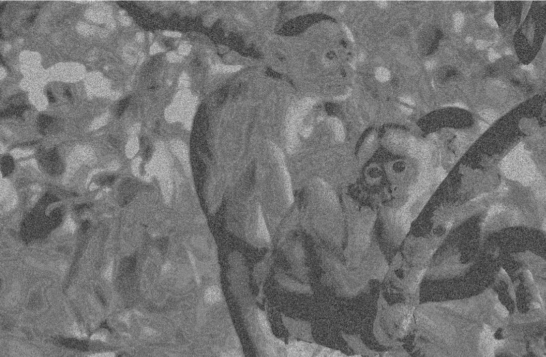
Figure 2: Encoded using a reflex-and-prefix algorithm; $p=0.2$.

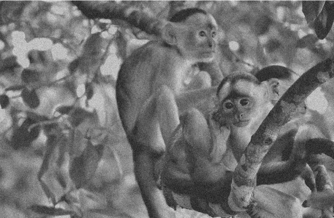
Figure 3: Encoded using a lexicographic order; $p=0.2$.

Simulations show that, in this situation, the lexicographic encoder seems to be optimal. In Figure 5, we consider the case $n=k=4$ and, in Figure 5, we consider the case $n=k=8$. On both graphs, the red lines represent the normalized expected loss attained by the lexicographic encoder (as a function of the overall error probability $p$). The other values correspond to different encoders, sampled randomly for different values of $p$.

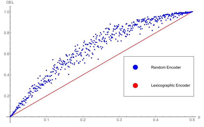
Figure 4: $n=k=4$

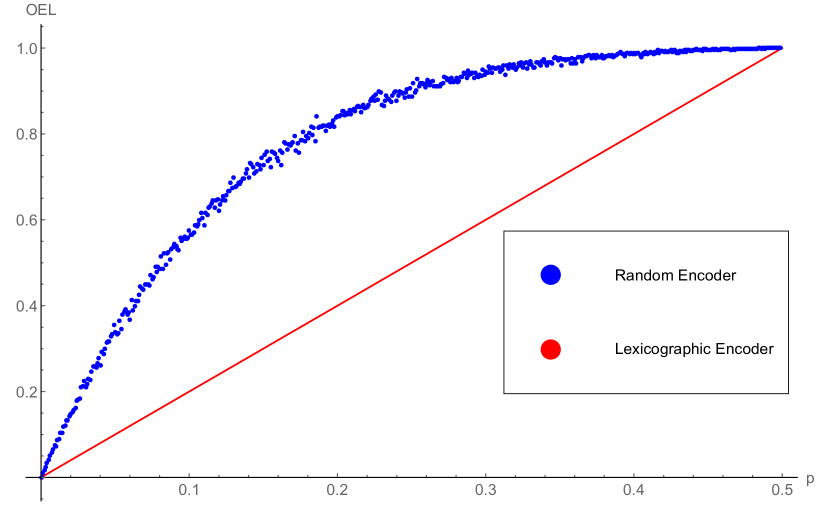
Figure 5: $n=k=8$

We remark that, when $n=k$ increases, the difference in the performance between the lexicographic encoder and a random encoder (in the average) also increases.

We generalize this approach when considering an information set $\mathcal{I}$ with $\left|\mathcal{I}\right|=2^{k}$ elements and a proper code $C$ in $\mathbb{\mathbb{F}}_{2}^{n}$ with $n\geq k$. We say an encoder $f:\mathcal{I}\rightarrow C$ is a lexicographic encoder if it satisfies the following condition: given $\iota_{j},\iota_{l}\in\mathcal{I}$, if $f\left(\iota_{j}\right)=x=\left(x_{1},\ldots,x_{n}\right)$ and $f\left(\iota_{l}\right)=y=\left(y_{1},\ldots,y_{n}\right)$, then

$$j<l\iff\sum_{i=1}^{n}x_{i}2^{i-1}<\sum_{i=1}^{n}y_{i}2^{i-1}\text{.}$$

We cannot prove that this is indeed a Bayes encoder, but experimental evidence supports this conjecture not only for the maximal likelihood (ML) decoder for the BMSC but also for various other encoders. Let us consider the situation described in our toy example where we have $2^{4}$ different tones of gray and let us consider an $\left[7;4\right]_{2}$ linear code $C$. We consider a decoder $a:\mathbb{F}_{2}^{7}\rightarrow C$ and compute the normalized expected loss function for different encoders and different values of $p$. On each of the pictures in Figures 7, 7, 9 and 9, we have that:

• The red line represents the lexicographic encoder;

• The black line represents an encoder $f:\mathcal{I}\rightarrow C$ such that, for $i\leq j$, we have $w_{H}\left(f\left(\iota_{i}\right)\right)\leq w_{H}\left(f\left(\iota_{j}\right)\right)$. Here, $w_{H}\left(\cdot\right)$ is the usual Hamming weight of a vector. Such an encoder is called a weight priority encoder and, its role will be explained by Theorem 3 in Section V ;

• The blue line represents an average (taken over all of the possible encoders) expected loss;

• The points represent random sampling of encoders for different values of $p$.

We consider two different $\left[7;4\right]_{2}$ codes $\mathcal{H}\left(3\right)$ and $\mathcal{C}\left(3\right)$ and two different decoders, $a_{ML}$ and $a_{T}$, such that each of those four pictures represents a pair $\left(C,a\right)=\left(\text{code,decoder}\right)$. The codes and decoders are the following:

• $\mathcal{H}\left(3\right)$ is the Hamming code with a parity check matrix

  $$\left(\begin{array}[c]{ccccccc}1&0&1&0&1&0&1\\ 0&1&1&0&0&1&1\\ 0&0&0&1&1&1&1\end{array}\right)\text{;}$$

• $\mathcal{C}\left(3\right)$ is the code with a generator matrix

  $$\left(\begin{array}[c]{ccccccc}1&0&0&0&1&0&1\\ 0&1&0&0&0&1&1\\ 0&0&1&0&1&1&0\\ 0&0&0&1&0&0&1\end{array}\right);$$

• $a_{ML}$ is the maximal likelihood decoder or the nearest (relative to the Hamming distance $d_{H}$) neighbor decoder;

• $a_{T}$ is the nearest neighbor decoder relatively to the metric $d_{T}\left(x,y\right):=\max\left\{i:x_{i}\neq y_{i}\right\}$, called the total-order decoder or just ordered decoder (more details about this decoder are explained in the next section).

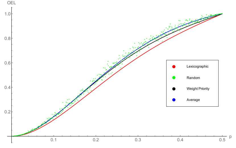
Figure 6: $(\mathcal{H}(3),a_{ML})$

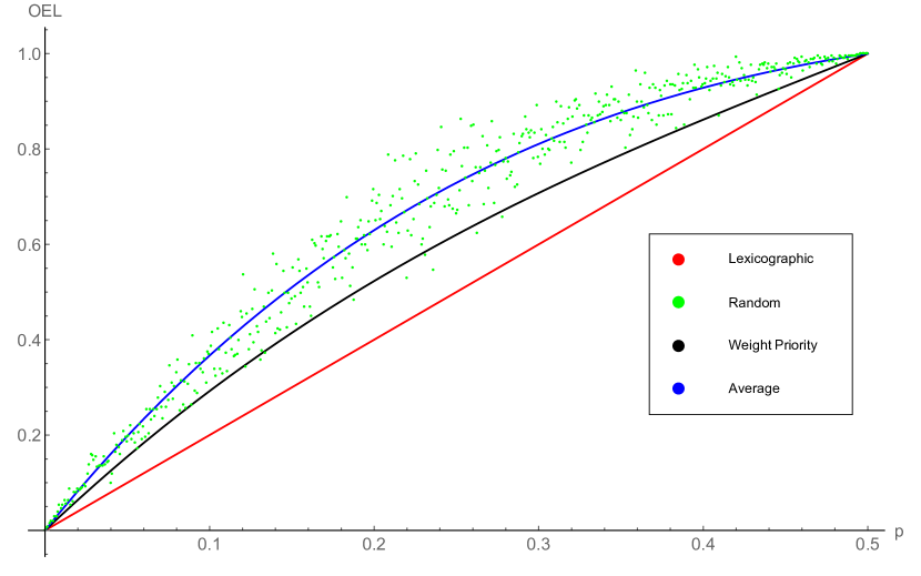
Figure 7: $(\mathcal{H}(3),a_{T})$

Figure 8: $(\mathcal{C}(3),a_{ML})$

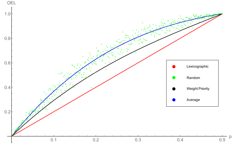
Figure 9: $(\mathcal{C}(3),a_{T})$

Those simulations support the conjecture that, for those decoders, the lexicographic encoder is a Bayes encoder.

IV-B Decoding

For the encoding part of the problem, we presented the lexicographic encoder as a candidate to be a Bayes encoder for a pair $\left(C,a\right)$, where $C$ is a linear code and $a$ is either the ML-decoder $a_{ML}$ or the decoder $a_{T}$ defined to be an NN-decoder (according to some metric quite different from the Hamming one).

For the decoding part of the problem, the situation is more blurry.

The approach adopted in this work is somewhat in the same direction that has been followed in various recent works regarding unequal error protection (UEP). The proposed use of nearest-neighbor decoders determined by a family of ordered metrics (that will be introduced on the sequence) is actually a decoding process that gives UEP of bits (bit-wise UEP), in a similar manner to that proposed in 1967 by Masnick and Wolf in [9] and since then extensively studied by many authors. Alternately, considering UEP of messages (message-wise UEP) is the approach adopted by Borade, Nakiboglu and Zheng in [3], where they consider the necessity of protecting in different ways pieces of information that are different in their nature (such as data and control messages) or have different types of errors (erasures and mis-decoded messages). This is performed by assigning larger decoding regions to the more valuable information.

Our approach is more general, and, in some sense, it combines message-wise and bit-wise UEP. We protect the messages by placing (encoding) similar (in the semantic sense) information messages close to each other and by adopting a decoding criterion that gives priority to the most significant bits.

We consider here two different metrics over $\mathbb{F}_{q}^{n}$, the usual Hamming distance $d_{H}$ and the total-order metric $d_{T}\left(x,y\right)=\max\left\{i:x_{i}\neq y_{i}\right\}$. Those two metrics are particular instances of the so-called hierarchical poset metrics (see, for example, [12] or [6] for an introduction to the subject) and when we do not need to distinguish between them, we may denote the metric as just $d_{P}$. As any metric, the metric $d_{P}$ determines a nearest neighbor (NN) decoder $a_{P}$: once a message $y$ is received $a_{P}\left(y\right)$ is chosen to minimize the distance to the code, that is, $a_{P}\left(y\right)\in\arg\min\left\{d_{P}\left(y,c\right):c\in C\right\}$. In the case of ambiguity (when $\left|\arg\min\left\{d_{P}\left(y,c\right):c\in C\right\}\right|\geq 2$), we assume the elements in $\arg\min\left\{d_{P}\left(y,c\right):c\in C\right\}$ are chosen randomly, with i.i.d. Thus, out of those two metrics, $d_{H}$ and $d_{T}$, we consider two different decoders $a_{H}$ and $a_{T}$. We remark that this definition of a decoder is actually a list-decoding type definition, and it coincides with the one presented in Section II only when $\left|\arg\min\left\{d_{P}\left(y,c\right):c\in C\right\}\right|=1$. When such an ambiguity exists, by considering an expected loss function, we will actually be considering the average (over all of the ambiguities) of the corresponding expected loss functions.

The idea of using hierarchical poset metrics lies in the fact that those metrics are matched to a lexicographic encoder, in the sense that it gives more protection against errors in the bits that become more significant due to the lexicographical manner of encoding. By using a decoder that is not ML, the number of errors (after decodification) increases, but not uniformly; less significant errors may increase a greatly, but more significant errors should decrease.

The main question is therefore the following: Is there a threshold where the loss of having more errors is compensated by the reduction in the most significant errors? We do not give a conclusive answer to this question but present some experimental evidence that shows it is indeed the case.

We consider the same toy example as in the encoding part, that is, we consider each pixel to be attributed a color chosen from a palette with $16$ gray tones. To explore the decoding side of the problem, we add redundancy by encoding each pixel as a codeword in the (perfect) $\left[7;4\right]_{2}$ binary Hamming code, one codeword assigned for each color that represents a pixel. Because the lexicographic encoder seems to be the Bayes encoder for both $a_{ML}$ and $a_{P}$, we consider it as fixed and start to compare decoders.

Using a random number generator, an error was created for each of the seven bits of each pixel, with an overall error probability of $p=0.35$. The same received picture was corrected twice, once using the usual ML decoder and once using an NN-decoder $a_{T}$, determined by the metric $d_{T}$.

To illustrate the performance of those decoders, we consider the same tamarins picture (Figure 1) as the original message. In Figure 10, all of the pixels that were correctly decoded are painted in purple, while the wrongly decoded pixels are left as decoded. On the left side, we see the result for the ML decoder, and on the right side, the result for the NN-decoder $a_{T}$.

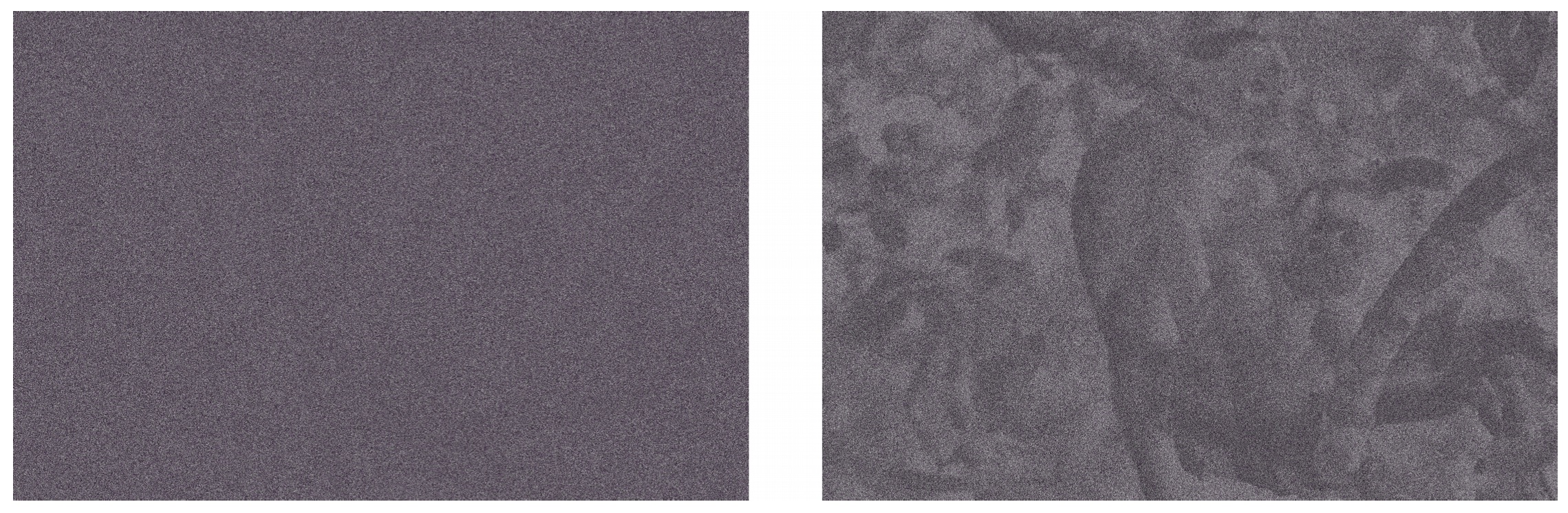
Figure 10: Right corrected pixels are colored with purple.

As expected, the picture on the left is much more color homogeneous (purple-like), because using ML to decode with a perfect code minimizes the amount of errors. However, one can identify the pixels to be painted in purple only when having the original picture. When looking at the picture as it was decoded using the two different decoding schemes, one gets a quite different perception:

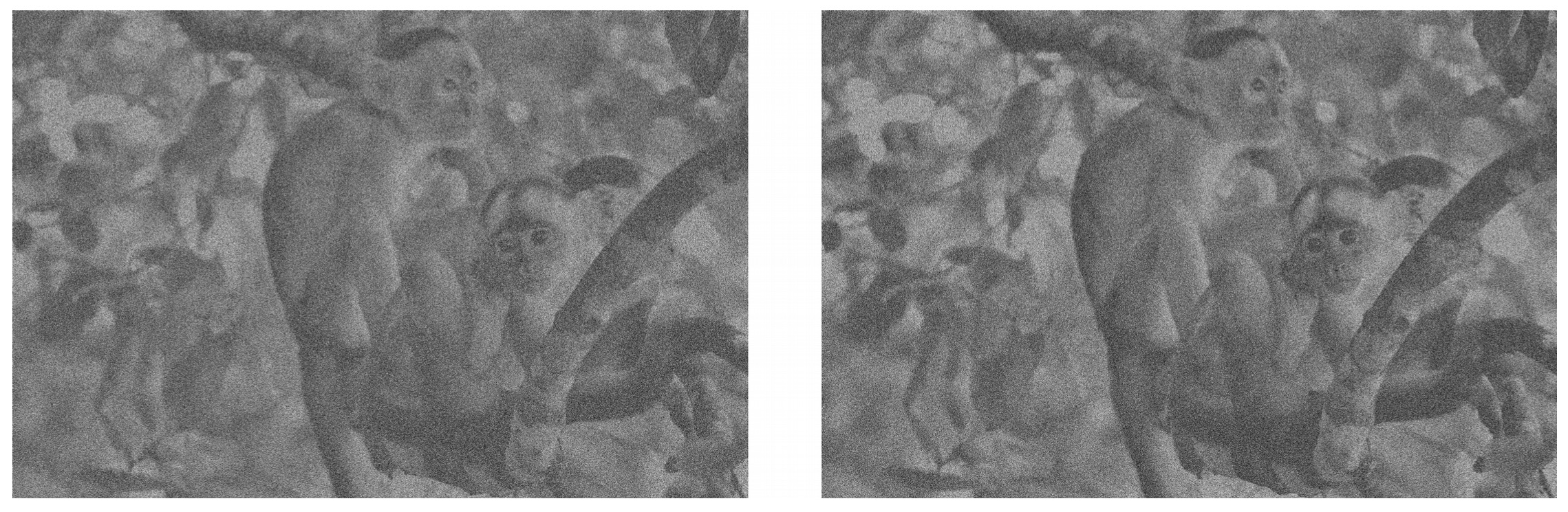
Figure 11: On the left, ML decoding, and, on the right, NN decoding; $p=0.35$.

The right-hand image seems to be sharper, closer to the original picture (Figure 11). This perception regarding the quality of these decoded pictures is an example of a way of valuing the error, in a situation in which each of us, ordinary viewers, may be considered as a type of expert.

In Figures 12 and 13 we can see that, even under a very high word error probability ($p=0.4$ and $p=0.43$), it is possible to grasp something of the original message.

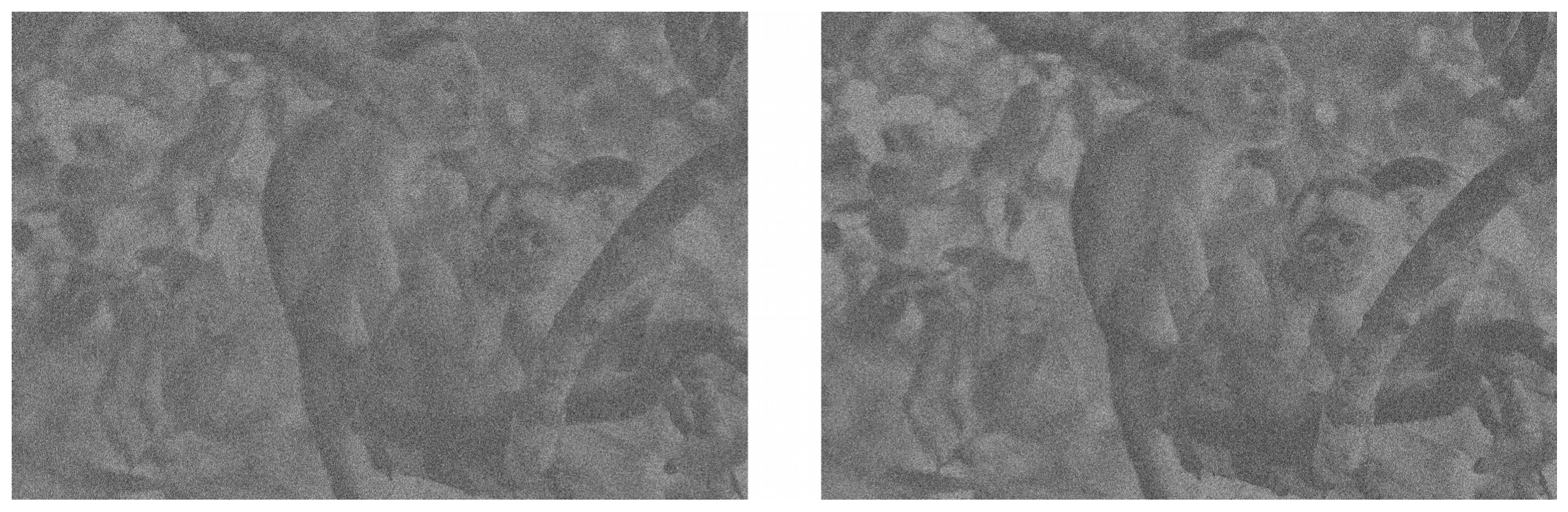
Figure 12: On the left ML decoding and on the right $T$-decoding; $p=0.4$.

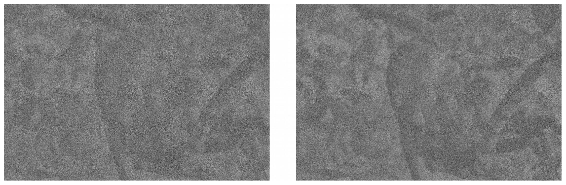
Figure 13: On the left ML decoding and on the right $T$-decoding; $p=0.43$.

We are able to compute expected loss for those small examples. In the pictures bellow we graph the expected loss functions in many situations. In each of them, we are considering one code and two decoders: the Hamming decoder $a_{H}$ in red and the total-order decoder $a_{T}$ in black). For each of those codes, we consider always an lexicographic encoder. The channel is considered to be a BMSC with overall error probability $p$ and the value function is the one determined by MSE.

Figure 14: Code $\mathcal{H}(3)$.

Figure 15: Code $\mathcal{C}(3)$.

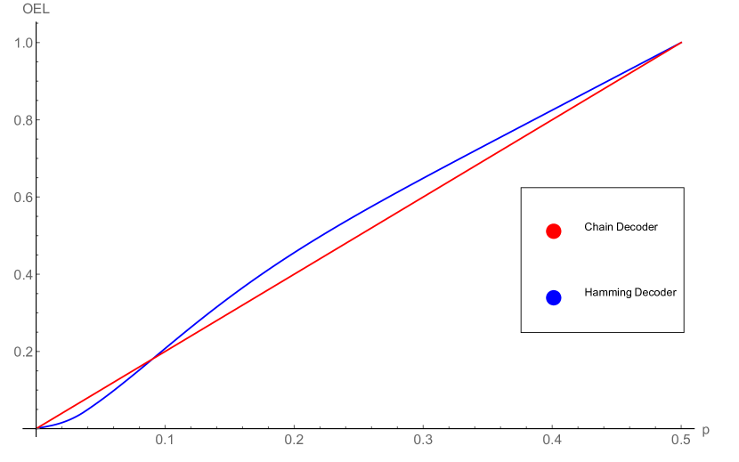
Figure 16: Code $\mathcal{H}(4)$.

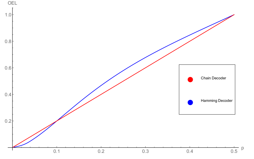
Figure 17: Code $\mathcal{C}(4)$.

The first two pictures represent the situation with $4$ bits of color (information) and the same redundancy, so we consider two $\left[7;4\right]_{2}$ linear codes: the Hamming code $\mathcal{H}\left(3\right)$ and the code $\mathcal{C}\left(3\right)$, both introduced in the end of Section IV-A. In the last two pictures, we consider $11$ bits of color (information) and the same redundancy, so we consider two $\left[15;11\right]_{2}$ linear codes: the Hamming code $\mathcal{H}\left(4\right)$ and the code $\mathcal{C}\left(4\right)$ that has a parity check matrix

$$\left(\begin{array}[c]{ccccccccccccccc}1&0&0&0&1&1&1&0&0&0&0&0&1&1&0\\ 0&1&0&0&0&1&0&1&1&1&0&1&0&1&0\\ 0&0&1&0&0&0&0&1&0&0&0&1&0&0&1\\ 0&0&0&1&0&0&0&0&0&1&0&1&0&1&1\end{array}\right)\text{.}$$

As we can see, for small $p$, the ML decoder seems to be the best choice. Nevertheless, those pictures depict the existence of a threshold $p_{0}$ above which the ordered decoders should be used. We do not know what would be the behavior of such a threshold for large $n$, but it seems that, for (very) noisy channels, using those ordered decoders may improve the performance and yield an extra bonus: very efficient decoding algorithms (details in [6]).

V Error Value Functions that are Invariant by Translations

In this section, we assume that the information set $\mathcal{I}$ is identified with the vector field $\mathbb{F}_{q}^{k}$, that is, we assume $\mathcal{I}=\mathbb{F}_{q}^{k}$, and we consider a special class of error value functions over $\mathbb{F}_{q}^{k}$, those that are invariant by translations. We assume also that $\mathcal{X}=\mathcal{Y}=\mathbb{F}_{q}^{n}$ and that $C$ is an $\left[n;k\right]_{q}$ linear code.

We say that an error value function $\nu:\mathbb{F}_{q}^{k}\times\mathbb{F}_{q}^{k}\rightarrow\mathbb{R}_{+}$ is invariant by translations if

$$\nu\left(x+z,y+z\right)=\nu\left(x,y\right)$$ (10)

for all $x,y,z\in\mathbb{F}_{q}^{k}$. In this case, we may consider a function $\widetilde{\nu}:\mathbb{F}_{q}^{k}\rightarrow\mathbb{R}_{+}$ (also called an error value function) defined by $\widetilde{\nu}\left(x\right):=\nu\left(x,0\right)$ because $\nu\left(x,y\right)=\nu\left(x-y,0\right)$.

We remark that, whenever there is a significant real number model for the information as an injective map $m:\mathcal{I}\rightarrow\mathbb{R}$, an error value function $\nu$ is said to be compatible with the model if $\mu\left(\iota_{1},\iota_{2}\right)$ is increasing with the difference $\left|m\left(\iota_{1}\right)-m\left(\iota_{2}\right)\right|$. It is not difficult to see that an error value function invariant by translations can not be compatible with a real number model for the information, and, in such a situation, a translation invariant error value function can be regarded only as a simplified model for errors. We also remark that, when defining invariance by translations, we assumed that the information set $\mathcal{I}$ is identified with the vector space $\mathbb{F}_{q}^{k}$, let us say by a bijection $\sigma:\mathcal{I}\rightarrow\mathbb{F}_{q}^{k}$. The identity (10) actually depends on $\sigma$, so that in fact we should say $\nu$ is $\sigma$-invariant invariant by translations. Nevertheless, we assume $\sigma$ is given and fixed, and hence the notation we adopt ignores its role.

The advantage of error value functions that are invariant by translations is that this allows us to determine Bayes encoders, as we see in the next two propositions.

As stated in equation (3), we express

$$\mathbb{E}\left(C,a,\nu_{f}\right)=\sum_{\left(c,c^{\prime}\right)\in C\times C}G_{a}\left(c,c^{\prime}\right)\nu_{f}\left(c,c^{\prime}\right)$$

where $G_{a}\left(c,c^{\prime}\right)=\sum_{y\in a^{-1}\left(c\right)}P\left(\left.c^{\prime}\right|y\right)P\left(y\right)$. Assuming now that the encoder $f:\mathbb{F}_{q}^{k}\rightarrow C$ is a linear map, we have that $\nu_{f}\left(c,c^{\prime}\right)=\nu_{f}\left(c-c^{\prime},0\right)=\widetilde{\nu}_{f}\left(c-c^{\prime}\right)$, and, writing $u=c-c^{\prime}$, we find that

$$\mathbb{E}\left(C,a,\nu_{f}\right) =\sum_{\left(c,c^{\prime}\right)\in C\times C}G_{a}\left(c,c^{\prime}\right)\widetilde{\nu}_{f}\left(c-c^{\prime}\right)$$

$$=\sum_{u\in C}\left(\sum_{c-c^{\prime}=u}G_{a}\left(c,c^{\prime}\right)\right)\widetilde{\nu}_{f}\left(u\right)$$

$$=\sum_{u\in C}\left(\sum_{c\in C}G_{a}\left(c,c-u\right)\right)\widetilde{\nu}_{f}\left(u\right)$$

and we get the following:

Proposition 1

If $\nu$ is an error value function invariant by translations and $f$ is a linear encoder, then

$$\mathbb{E}\left(C,a,\nu_{f}\right)=\sum_{c\in C}H_{a}(c)\widetilde{\nu}_{f}\left(c\right)$$

where

$$H_{a}(c):=\sum_{c\in C}G_{a}\left(c,c-u\right)=\sum_{y\in\mathbb{F}_{q}^{n}}P\left(a(y)-c|y\right)P(y).$$

We remark that $\mathbb{E}\left(C,a,\nu_{f}\right)$ is a linear combination of the values $\widetilde{\nu}_{f}\left(c\right)$, $c\in C$, and that the coefficients $H_{a}(c)$ do not depend on the encoder $f$. Because the values $\widetilde{\nu}_{f}\left(c\right)$ are all non-negative, it is simple to minimize the expected loss; one should choose an encoder $f$ that associates more valuable errors (higher $\widetilde{\nu}_{f}\left(c\right)$) to the lower coefficients $H_{a}(c)$.

Theorem 3

Let $C=\left\{c_{1},\ldots,c_{M}\right\}$ be a linear code, $a:\mathbb{F}_{q}^{n}\rightarrow C$ a decoder and $\nu:\mathbb{F}_{q}^{k}\times\mathbb{F}_{q}^{k}\rightarrow\mathbb{R}_{+}$ an error value function invariant by translations. We assume without loss of generality that

$$H_{a}\left(c_{1}\right)\geq H_{a}\left(c_{2}\right)\geq\ldots\geq H_{a}\left(c_{M}\right).$$

Then, a linear encoder $f:\mathbb{F}_{q}^{k}\rightarrow C$ is a Bayes encoder for the error value function $\nu$ and the decoder $a$ if and only if

$$\widetilde{\nu}_{f}\left(c_{1}\right)\leq\widetilde{\nu}_{f}\left(c_{2}\right)\leq\cdots\leq\widetilde{\nu}_{f}\left(c_{M}\right)\text{.}$$

From here on, we assume that the prior probability of $C$ is uniform.

We now explore an example that illustrates the preceding results for the case of a perfect code. Let us assume the channel to be a binary memoryless symmetric channel with overall error probability $p$. Let $w_{H}(c):=d_{H}\left(c,0\right)$ be the Hamming weight of $c$ and let $supp(x):=\{i:x_{i}\neq 0\}$ be the support of the vector $x=(x_{1},\ldots,x_{n})$.

Let $\mathcal{H}(l)$ be the $\left[n;k\right]_{2}$ binary Hamming code, where $n=2^{l}-1$ is the length of the block and $k=2^{l}-1-l$ the dimension of the code. Let $a:\mathbb{F}_{2}^{n}\rightarrow\mathcal{H}(l)$ be an ML decoder, so that $d_{H}\left(y,a\left(y\right)\right)\leq d_{H}\left(y,c\right)$, for all $y\in\mathbb{F}_{2}^{n}$ and every $c\in\mathcal{H}\left(l\right)$. In this situation, direct computations show that

$$H_{a}\left(c\right)=\frac{\left(1-p\right)^{n}}{M}\sum_{y\in\mathbb{F}_{2}^{n}}s^{d_{H}\left(y,a\left(y\right)-c\right)}$$ (11)

where $s:=\frac{p}{1-p}$ and $M:=\left|\mathcal{H}(l)\right|$. Since $\mathcal{H}\left(l\right)$ is a perfect code that corrects a single error and $a$ is an ML decoder, we find that either $y=a\left(y\right)$ or $y-a\left(y\right)=e_{i}$, a vector with Hamming weight $w_{H}\left(e_{i}\right)=1$. This ensures that

$$d_{H}\left(y,a\left(y\right)-c\right)=\left\{\begin{array}[c]{cc}w_{H}\left(e_{i}+c\right)&\text{for some }1\leq i\leq N\text{ if }y\notin\mathcal{H}\left(l\right)\\ w_{H}\left(c\right)&\text{ otherwise}\end{array}\right.\text{.}$$

We write

$$\sum_{y\in\mathbb{F}_{2}^{n}}s^{d_{H}\left(y,a\left(y\right)-c\right)} =\sum_{y\in\mathcal{H}\left(l\right)}s^{d_{H}\left(y,a\left(y\right)-c\right)}+\sum_{y\notin\mathcal{H}\left(l\right)}s^{d_{H}\left(y,a\left(y\right)-c\right)}$$

$$=\sum_{y\in\mathcal{H}\left(l\right)}s^{w_{H}\left(c\right)}+M\cdot\sum_{i\notin\text{\emph{supp}}\left(c\right)}s^{w_{H}\left(e_{i}+c\right)}+M\cdot\sum_{i\in\text{\emph{supp}}\left(c\right)}s^{w_{H}\left(e_{i}+c\right)}\text{.}$$

Because

$$\sum_{i\notin\text{\emph{supp}}\left(c\right)}s^{w_{H}\left(e_{i}+c\right)}=\left(n-w_{H}\left(c\right)\right)s^{w_{H}\left(c\right)+1}$$

and

$$\sum_{i\in\text{\emph{supp}}\left(c\right)}s^{w_{H}\left(e_{i}+c\right)}=w_{H}\left(c\right)s^{w_{H}\left(c\right)-1}\text{,}$$

considering expression (11), it follows that

$$H_{a}\left(c\right)=\left(1-p\right)^{n}(s^{w_{H}\left(c\right)}+\left(n-w_{H}\left(c\right)\right)s^{w_{H}\left(c\right)+1}+w_{H}\left(c\right)s^{w_{H}\left(c\right)-1})\text{,}$$

which depends only on $w_{H}\left(c\right)$ but not on $c$. Now it is possible to show that, for the Hamming code $\mathcal{H}\left(l\right)$, $H_{a}\left(c\right)\geq H_{a}\left(c^{\prime}\right)$ if $w_{H}\left(c\right)\leq w_{H}\left(c^{\prime}\right)$. Using this and Theorem 3, it follows that $f:\mathbb{F}_{2}^{k}\rightarrow\mathcal{H}\left(l\right)$ is a Bayes encoder of a Hamming code iff

$$\widetilde{\nu}_{f}\left(c\right)\leq\widetilde{\nu}_{f}\left(c^{\prime}\right)\text{ whenever }w_{H}\left(c\right)\leq w_{H}\left(c^{\prime}\right)\text{.}$$ (12)

Similar reasoning may be used to compute the coefficients $H_{a}\left(c\right)$ of the perfect $[23;12]_{2}$ Golay code and to show that condition (12) holds also for this code. We call such an encoder a weight priority encoder.

Finally, in addition to giving a good description of Bayes encoders, the use of a value function that is invariant by translation may be justified also by the fact that it generalizes two well-known measures of loss. When introducing the expected loss in Section II, we already showed that the word error probability may be considered as a particular instance of an expected loss function (by considering the indicator function $\nu_{0\text{-}1}$ to be the loss function). If we assume now that the channel is invariant by translations, in the sense that

$$P\left(\left.y\right|x\right)=P\left(\left.y+z\right|x+z\right)$$

for all $x,y,z\in\mathbb{F}_{q}^{n}$, we may look also at the bit error probability $P_{b}(C)$ of $C$ (BER) as a particular case of the expected loss function. This is attained by considering a decoder $a:\mathbb{F}_{q}^{n}\rightarrow C$ that is also invariant by translations, in the sense that

$$a^{-1}\left(c\right)=c+a^{-1}\left(0\right)$$

for every $c\in C$, considering any encoder $f:\mathbb{F}_{q}^{k}\rightarrow C$ and the value function $\nu:\mathbb{F}_{q}^{k}\rightarrow\mathbb{R}_{+}$ defined by

$$\nu_{f}\left(c\right)=\frac{w_{H}\left(f^{-1}\left(c\right)\right)}{k}\text{.}$$

The proof follows by direct calculations and comparison with the expression for BER, as given, for example, in [2].

References

[1]R. B. Ash - Information Theory - Dover Publication (1999).
[2]S. Benedetto and E. Biglieri - Principles of Digital
Transmission With Wireless Application - Klumer Academic (1999).
[3]S. Borade, B Nakiboğlu and L. Zheng - Unequal error
protection: an information-theoretic perspective - IEEE Transactions on
Information Theory (2009), vol. 55, No. 12, 5511-5539.
[4]R. Brualdi, J. S. Graves and M. Lawrence - Codes with
a poset metric - Discrete Mathematics 147 (1995) 57-72.
[5]T. Cover and J. A. Thomas - Elements of Information
Theory - John Wiley & Sons (2006).
[6]L. V. Felix and M. Firer - Canonical-Systematic Form of
Hierarchical Codes - Advances in Mathematics of Communications (2012) vol. 6,
No. 3, 315-328.
[7]K. Po Ho and J. M. Kahn - Image Transmission over
Noisy Channels Using Multicarrier Modulation - Signal Processing: Image
Communication 9 (1997) 159-169.
[8]H. K. Kim and D. Y. Oh - A Classification of Poset
Admitting the MacWilliams Identity - IEEE Transactions on Information Theory
(2005), vol. 51, No. 4, 1424-1431.
[9]B. Masnick and J. Wolf - On linear unequal error protection
codes - IEEE Transactions on Information Theory (1967), vol. 3, No. 4, 600-607.
[10]S. M. Moser - Weak Flip Codes and Applications to
Optimal Code Design on the Binary Erasure Channel - research report available
at http://moser-isi.ethz.ch/docs/papers/smos-2013-6.pdf, 2013.
[11]Po-Ning Chen, Hsuan-Yin Lin and S. M. Moser - Optimal
Ultrasmall Block-Codes for Binary Discrete Memoryless Channels - IEEE Transactions on Information Theory (2013), vol.59, No. 11, 7346-7378.
[12]L. Panek, M. Firer, H. Kwang Kim and J. Yoon Hyun -
Groups of linear isometries on poset structures - Discrete Mathematics
308 (2008) 4116-4123.
[13]L. Panek, M. Firer and M. M. S. Alves - Classification of
Niederreiter-Rosenbloom-Tsfasman Block Codes - IEEE Transactions on
Information Theory (2010), vol. 56, No. 10, 5207-5216.
[14] J. Walker and M. Firer, Matched Metrics and Channels, preprint, 2014.