A generalized mixed model framework for assessing fingerprint individuality in presence of varying image quality

Abstract

Fingerprint individuality refers to the extent of uniqueness of fingerprints and is the main criteria for deciding between a match versus nonmatch in forensic testimony. Often, prints are subject to varying levels of noise, for example, the image quality may be low when a print is lifted from a crime scene. A poor image quality causes human experts as well as automatic systems to make more errors in feature detection by either missing true features or detecting spurious ones. This error lowers the extent to which one can claim individualization of fingerprints that are being matched. The aim of this paper is to quantify the decrease in individualization as image quality degrades based on fingerprint images in real databases. This, in turn, can be used by forensic experts along with their testimony in a court of law. An important practical concern is that the databases used typically consist of a large number of fingerprint images so computational algorithms such as the Gibbs sampler can be extremely slow. We develop algorithms based on the Laplace approximation of the likelihood and infer the unknown parameters based on this approximate likelihood. Two publicly available databases, namely, FVC2002 and FVC2006, are analyzed from which estimates of individuality are obtained. From a statistical perspective, the contribution can be treated as an innovative application of Generalized Linear Mixed Models (GLMMs) to the field of fingerprint-based authentication.

T1Supported in part by NSF Grant SES-0961649, NSF Grant DMS-11-06450 and Universiti Teknologi PETRONAS URIF Grant no. 16/2013.

, and

1 Introduction

1.1 Fingerprint features, matching and individuality

Fingerprint individuality is the study of the extent of uniqueness of fingerprints and is the central premise for expert testimony in court. Assessment of individuality is made based on comparing features from two fingerprint images such as in Figure 1. A fingerprint image consists of alternating dark and light smooth flow lines termed as ridges and valleys. The fingerprint feature formed when a ridge occasionally either terminates or bifurcates is called a minutia; the minutia type “ending” and “bifurcation” correspondingly relate to the type of ridge anomaly that occurs. The location of a minutia is denoted by $x$ where $x\in D$, $D$ is the image domain. Figure 1 identifies all minutiae as white squares in the two fingerprint images; the images are from the publicly available database FVC2002. Each white line emanating from the center of the square represents the minutia direction, denoted by $u$ with $u\in(0,2\pi]$, which is (i) the direction of the merged ridge flow for a minutia bifurcation, and (ii) the direction pointing away from the ridge flow for a minutia ending; see Figure 1. Minutia information of a fingerprint consists of the collection of locations and directions, $(x,u)$, of all minutiae in the image.

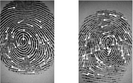
Figure 1: A total of $35$ and $49$ minutiae were detected in left and right images, respectively, and $w=7$ correspondences (i.e., matches) were found. The white squares and lines, respectively, represent the minutia location and direction. Note that for a minutia ending, the white line points away from the ridge flow, whereas for a minutia bifurcation, the white line points along the direction of the merged ridge. Images taken from the publicly available database FVC2002 DB2.

Minutiae in fingerprint images are extracted using pattern recognition algorithms. In this paper, we used the algorithm described in Zhu, Dass and Jain (2007) for minutia extraction. Minutia information is easy to extract, and believed to be permanent and unique; that is, minutiae information is believed to stay the same over time and different individuals have distinct minutia patterns, thus making it a popular method for identifying individuals in the forensics community. For a pair of prints, a minutia $(x,u)$ in one print is said to match a minutia $(y,v)$ in the another print if

$$|x-y|_{d}<r_{0}\quad\mbox{and}\quad|u-v|_{a}<u_{0}$$ (1)

for prespecified small positive numbers $r_{0}$ and $u_{0}$, where $|x-y|_{d}$ and $|u-v|_{a}$, respectively, denote the Euclidean distance in $R^{2}$ and the angular distance

$$|u-v|_{a}=\operatorname{min}\bigl{\{}|u-v|,2\pi-|u-v|\bigr{\}}.$$ (2)

We subsequently assume that a set of minutiae has already been extracted (or detected) for every fingerprint image under study. Fingerprint-based authentication proceeds by determining the highest possible number of minutia matches between a pair of prints. This is achieved by an optimal rigid transformation that brings the two sets of minutiae as close to each other as possible and then counting the number of minutia pairs $(x,u)$ and $(y,v)$ that satisfy (1). For example, the number of minutia matches between the prints in the left and right panels in Figure 1 is $w\equiv 7$.

A reasonably high degree of match (high $w$) between the two sets of minutiae leads forensic experts to testify irrefutably that the owner of the two prints is one and the same person. Central to establishing an identity based on fingerprint evidence is the assumption of discernible uniqueness; fingerprint minutiae of different individuals are observably different and, therefore, when two prints share many common minutiae, the experts conclude that the two different prints are from the same person. The primary concern here is what constitutes a “reasonably high degree of match?” For example, in Figure 1, is $w=7$ large enough to conclude that the two prints come from the same person? When fingerprint evidence is presented in a court, the testimony of experts is almost always included and, on cross-examination, the foundations and basis of this testimony are rarely questioned. However, in the case of Daubert vs. Merrell Dow Pharmaceuticals (1995), the U.S. Supreme Court ruled that in order for expert forensic testimony to be allowed in courts, it had to be subject to the criteria of scientific validation [see Pankanti, Prabhakar and Jain (2002) for details]. Following the Daubert ruling, forensic evidence based on fingerprints was first challenged in the case of U.S. vs. Byron C. Mitchell (1999) and, subsequently, in 20 other cases involving fingerprint evidence. The main concern with an expert’s testimony as well as admissibility of fingerprint evidence is the problem of individualization. The fundamental premise for asserting the extent to which the prints match each other (i.e., the extent of uniqueness of fingerprints) has not been scientifically validated and matching error rates are unknown [Pankanti, Prabhakar and Jain (2002), Zhu, Dass and Jain (2007)]; see also the National Academy of Sciences (NAS) report (2009).

The central question in a court of law is “What is the uncertainty associated with the experts’ judgement when matches are decided by fingerprint evidence?” How likely can an erroneous decision be made for the given latent print? The main issue with expert testimony is the lack of quantification of this uncertainty in the decision. To address these concerns, several research investigations have proposed measures that characterize the extent of fingerprint individuality; see Pankanti, Prabhakar and Jain (2002), Zhu, Dass and Jain (2007) and the references therein. The primary aim of these measures is to capture the inherent variability and uncertainty (in the expert’s assessment of a “match”) when an individual is identified based on fingerprint evidence.

A measure of fingerprint individuality is given by the probability of a random correspondence (PRC), which is the probability that two sets of minutiae, one from the query containing $m_{1}$ minutiae and the other from the template fingerprint containing $m_{2}$ minutiae, randomly correspond to each other with at least $w$ matches. Since large (resp., small) $w$ is a measure of the extent of similarity (resp., dissimilarity) between a pair of fingerprints, the PRC should be a decreasing function of $w$. Mathematically, the PRC corresponding to $w$ matches is given by

$$\operatorname{PRC}(w|m_{1},m_{2})=P(\mathcal{S}\geq w|m_{1},m_{2}),$$ (3)

where the random variable $\mathcal{S}$ denotes the number of minutia matches that result when two arbitrary fingerprints from a target population are paired with each other; the notation used in (3) also emphasizes the dependence of the PRC on the total number of minutiae detected in the two prints, that is, $m_{1}$ and $m_{2}$. It is clear from the above formula that $\operatorname{PRC}(w|m_{1},m_{2})$ decreases as $w$ increases for fixed $m_{1}$ and $m_{2}$. The distribution of $\mathcal{S}$ is governed by the extent to which minutia matches occur randomly, an unknown quantity which has been modeled in a variety of ways in the literature. The main aim of research in fingerprint individuality is to obtain reliable inference on the PRC, which is also unknown as a result of the unknown extent of random minutia matches.

1.2 Minutia matching models

Several fingerprint minutia matchingmodels and expressions for the PRC have been developed from a completely theoretical perspective [see Pankanti, Prabhakar and Jain (2002) for a detailed account of these models]. These models are distributions elicited for minutia occurrences, that is, the distributions that arise from viewing each minutia $(x,u)$ as a random occurrence in the fingerprint, occurring independently of each other. A major drawback of these works is that the models for minutia occurrences, and consequently matching probabilities and PRCs, are not validated based on actual fingerprint images. This effort was first carried out in Pankanti, Prabhakar and Jain (2002) based on real fingerprint databases, albeit for a simple minutia matching model. Subsequent improvements on validating matching models based on actual fingerprint databases have been carried out in Zhu, Dass and Jain (2007) and several other works. Zhu, Dass and Jain (2007), for example, demonstrated that when the number of minutiae in the prints are moderate to large, the distribution of $\mathcal{S}$ in (3) can be approximated by a Poisson distribution with mean $\lambda$, the expected number of random matches, given by

$$\lambda=\lambda(f_{1},f_{2})=m_{1}m_{2}\biggl{(}2\pi r_{0}^{2}u_{0}\int_{D}\int_{(0,2\pi]}f_{1}(x,u)f_{2}(x,u)\,dx\,du\biggr{)},$$ (4)

based on the minutia distributions $f_{1}$ and $f_{2}$ for prints $1$ and $2$, respectively; in (4), $m_{1}$ and $m_{2}$ are, respectively, the number of minutiae in prints $1$ and $2$, and $r_{0}$ and $u_{0}$ are as in (1). The above formula for the mean number of random matches can be understood in the following way: The total number of pairings available for random matching from $m_{1}$ minutiae in print $1$ and $m_{2}$ minutiae in print $2$ is $m_{1}m_{2}$. The expression $2\pi r_{0}^{2}u_{0}\int_{D}\int_{(0,2\pi]}f_{1}(x,u)f_{2}(x,u)\,dx\,du$ represents the probability of a single random match when $r_{0}$ and $u_{0}$ are small compared to the image size. It follows from the expected value of a binomial distribution that $\lambda$ in (4) is the mean number of successes (i.e., random matches). The contribution of Zhu, Dass and Jain (2007) was to characterize the distribution of $\mathcal{S}$ (the extent of random matching in the target population) by a single number, namely, the probability of a (single) random match between two minutiae, one from each of the prints in question. Since the probability of a random match

$$p(f_{1},f_{2})=2\pi r_{0}^{2}u_{0}\int_{D}\int_{(0,2\pi]}f_{1}(x,u)f_{2}(x,u)\,dx\,du$$ (5)

depends on the minutia distributions $f_{1}$ and $f_{2}$, Zhu, Dass and Jain (2007) inferred these distributions from actual fingerprint databases by representing them as a finite mixture of normals.

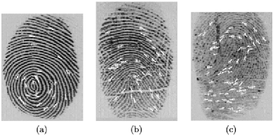
Figure 2: Fingerprint images with (a) good (b) moderate and (c) poor quality. White squares and lines indicate locations and directions of detected minutiae, and possibly not true ones in panel (c); images taken from the publicly available FVC2002 databases.

Factors other than the minutia distributions also govern the extent of random matches. In the case of forensic testimony, for example, it is reasonable to believe that expert matching is more prone to error if the latent prints are of poor quality. Here, poor quality images mean poor resolution (or clarity) of the ridge-valley structures (e.g., in the presence of smudges, sweaty fingers, cuts and bruises) due to which the detection of true minutiae can be missed and spurious minutiae can be detected; see Figure 2 for examples of good, moderate and poor quality fingerprint images. In other words, the extent of individualization should be smaller when the underlying image qualities are poor. One critical issue, therefore, is to be able to quantify the increase in PRC with respect to quality degradation for each matching number $w$. This quantification is crucial, for example, for latent prints lifted from crime scenes which are known to have inferior image quality. In the presence of poor quality, automatic as well as manual extraction of fingerprint features are prone to more errors through (i) increased likelihood of detecting spurious minutiae and (ii) missing true ones. Previous work has not quantified the effects of (i) and (ii) on fingerprint individuality; see Dass (2010).

1.3 Objective and contributions

The aim of this paper is to quantify PRC assessment (and hence fingerprint individuality) in the presence of varying image quality. The methodology involves two main steps. (i) First, a class of generalized linear mixed models (GLMMs) is proposed that consists of two levels. At the top level, the Poisson model is elicited as the distribution for the number of random minutia matches, following the derivation of Zhu, Dass and Jain (2007). At the second level, image quality of the two prints in question are incorporated as covariates. Also, inter-finger variability is modeled using variance components in the second level. (ii) Second, an inference procedure for the PRC is developed to accommodate a large number of images from different fingers as is typical in real fingerprint databases. Efficient computational algorithms are essential for arriving at reliable reports of fingerprint individuality in practice. Since the number of fingerprint images in real databases is typically large, inference based on Bayesian computational algorithms such as the Gibbs sampler is extremely slow due to increased dimensions of the parameter space. To alleviate this problem, the asymptotic Laplace approximation of the GLMM likelihood is used instead. To summarize, contributions of this paper are as follows: For fingerprint-based authentication, a procedure is developed for obtaining the PRC based on explicitly modeling the occurrence of spurious minutia on image quality degradation. Statistical contributions include (i) an innovative application of GLMM to fingerprint-based authentication, and (ii) the development of computationally fast algorithms achieved by approximating the GLMM likelihood (with associated theoretical and numerical validation). Inference results (point estimates and credible intervals) on the PRC are also given (see the experimental results section—Section 6).

The rest of this paper is organized as follows: Section 3 discusses the log-linear GLMM model that is used to study how PRCs change as a function of the underlying image quality. Section 4 presents the procedure for fitting GLMMs in a Bayesian framework. Section 5 develops the inference procedure (point estimates and credible intervals) on the PRC. Section 6 obtains the estimates of fingerprint individuality based on the FVC2002 and FVC2006 databases and gives an analysis of the numerical results. Section 7 validates the Laplace approximation and various other approximations used in this paper for efficient computation. Section 8 presents the summary, conclusions and other relevant discussions.

2 Fingerprint databases and empirical findings

2.1 Fingerprint databases

Fingerprint databases that have been used in fingerprint analysis include the FVC (e.g., FVC2000, 2002, 2004 and 2006) and NIST databases (e.g., NIST Special Database 4, 9, 27, etc.) which are publicly available for download and analysis. These fingerprint databases typically consist of images acquired from $F$ different fingers, obtained by placing the finger onto the sensing plate of an image acquisition device. Each finger is sensed multiple times, possibly a different number of times for the different fingers. The databases have a common number of multiple acquisitions, say, $L$, for each finger, resulting in total of $FL$ images in the database. Due to the different sensors used as well as varying placement of the finger, per individual, onto the sensing plate, the images acquired exhibit significant variability (even for the same finger); see Figure 3 for several examples from two of the databases used in this paper, namely, FVC2002 (DB1 and DB2) and FVC2006 (DB3). For FVC2002 DB1 and DB2, $F=100$ and $L=8$, whereas for FVC2006 DB3, $F=150$ with $L=15$. Figure 3 gives an idea of the intra-finger variability (variability due to multiple impressions) that has to be taken into account in addition to image quality variability. Intra-finger variability gives different matching numbers when different impressions are used for the matching between two fingers.

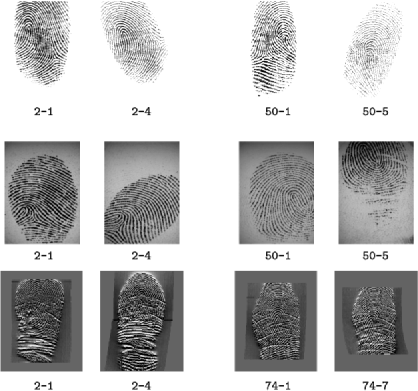
Figure 3: Sample images from the FVC2002 DB1, DB2 and FVC2006 DB3 databases; impression $f\mbox{--}l$ refers to the $l$th impression of the $f$th finger. Top, middle and bottom rows are images from the FVC2002 DB1, DB2 and FVC2006 DB3 databases, respectively; all images are publicly available.

2.2 Empirical findings for varying image quality

In practice, the quality of an image can be either ordinal (i.e., taking values in an ordered label set) or quantitative (i.e., taking values in a continuum, usually in a bounded interval $[a,b]$). We have considered one specific choice of each type of quality measure: (i) The categorical quality extractor “NFIQ,” which is an implementation of the “NIST Image Quality” algorithm based on neural networks described in Tabassi, Wilson and Watson (2004), and (ii) the minutia quality extractor obtained from the feature extraction algorithm mindtct from NIST (see the Home Office Automatic Fingerprint Recognition System [HOAFRS (1993)]). These algorithms are all publicly available. For the NFIQ quality extractor, the output $Q_{0}$ is a quality label numbered $1,2,\ldots,5$, with $1$ and $5$ corresponding to the best and worst quality images, respectively. For the continuous quality extractor by mindtct, a real number $Q_{\mathrm{con}}$ between $0$ and $1$ is obtained with higher values indicating better quality images. To maintain consistency between the two quality measures, we relabel the categorial measure as $Q_{\mathrm{cat}}=Q_{\mathrm{max}}+1-Q_{0}$, where $Q_{\mathrm{max}}$ is the maximum label for a given database, so that higher labels indicate better quality images.

For a pair of prints, $1$ and $2$ say, with $m_{1}$ and $m_{2}$ minutiae, respectively, let $Y$ denote the observed number of minutia matches between them. We consider only impostor matches (matches between impressions of different fingers) which are equivalent to the notion of random matching when assessing fingerprint individuality. The total number of impostor pairs in a database with $F$ fingers and $L$ impressions per finger is $F(F-1)L^{2}/2$ (since the order of the prints is immaterial). Suppose $(Q_{1},Q_{2})$ are the labels for the categorical measure $Q_{{\mathrm{cat}}}$. Table 1 gives the average number (and standard deviations) of matches $\bar{Y}$ for each quality bin pair based on FVC2002 DB1 and DB2. Note that the average number of matches is an increasing function of the quality labels, that is, the average number of random matches increases as the image quality becomes better. This seems counterintuitive initially, but we note that the average increases because the total number of minutiae extracted from the two prints also increases as quality gets better. With more minutiae available for random pairings, the number of matches based on such pairings should also increase on the average. Table 2 gives the mean number (and standard deviations) of minutiae for each quality bin for the two databases considered to illustrate this trend. The minutia extraction algorithm mindtct detects (or extracts) a minutia only if its computed reliability measure (computed within the program) is above a certain threshold. For better quality images, more minutiae have a reliability index above the threshold, which explains the higher number extracted in better quality images.

Table 1: Mean and standard deviations (in parenthesis) of $Y$ (the observed number of random matches) for $Q_{\mathrm{cat}}$ pairs for FVC2002 DB1 and DB2 in panels (a) and (b)

$\bolds{Q_{1}/Q_{2}}$ $\bolds{1}$ $\bolds{2}$ $\bolds{3}$ $1$ 3.36 3.43 4.15 (1.11) (1.14) (1.36) $2$ 3.73 4.02 4.94 (1.13) (1.19) (1.41) $3$ 4.57 4.96 6.38 (1.40) (1.43) (1.71)	$\bolds{Q_{1}/Q_{2}}$ $\bolds{1}$ $\bolds{2}$ $\bolds{3}$ $\bolds{4}$ $1$ 2.20 3.02 3.36 3.76 (0.42) (0.76) (0.90) (1.00) $2$ 2.96 3.91 4.21 5.12 (0.75) (1.30) (1.39) (1.71) $3$ 3.19 4.26 4.71 5.77 (0.82) (1.26) (1.32) (1.57) $4$ 3.74 5.26 5.96 7.47 (0.99) (1.51) (1.58) (1.91)
(a)	(b)

Table 2: Mean and standard deviations (in parenthesis) of $m_{1}m_{2}$ (the total number of possible random pairings) for $Q_{\mathrm{cat}}$ pairs for FVC2002 DB1 and DB2 in panels (a) and (b)

$\bolds{Q_{1}/Q_{2}}$ $\bolds{1}$ $\bolds{2}$ $\bolds{3}$ $1$ 357 403 641 (239) (219) (336) $2$ 490 594 947 (260) (221) (327) $3$ 768 921 1459 (383) (301) (440)	$\bolds{Q_{1}/Q_{2}}$ $\bolds{1}$ $\bolds{2}$ $\bolds{3}$ $\bolds{4}$ $1$ 177 366 482 705 (53) (144) (148) (203) $2$ 338 684 835 1295 (178) (395) (445) (634) $3$ 414 845 1036 1596 (138) (368) (350) (485) $4$ 650 1342 1682 2546 (192) (527) (491) (655)
(a)	(b)

Table 3: Mean and standard deviations (in parenthesis) of $Y/(m_{1}m_{2})$ (the probability of a random pairing) for $Q_{\mathrm{cat}}$ pairs for FVC2002 DB1 and DB2 in panels (a) and (b)

$\bolds{Q_{1}/Q_{2}}$ $\bolds{1}$ $\bolds{2}$ $\bolds{3}$ $1$ 0.0127 0.0105 0.0077 (0.0083) (0.0057) (0.0036) $2$ 0.0092 0.0075 0.0056 (0.0046) (0.0030) (0.0019) $3$ 0.0069 0.0058 0.0046 (0.0029) (0.0018) (0.0013)	$\bolds{Q_{1}/Q_{2}}$ $\bolds{1}$ $\bolds{2}$ $\bolds{3}$ $\bolds{4}$ $1$ 0.0131 0.0090 0.0074 0.0056 (0.0032) (0.0029) (0.0024) (0.0021) $2$ 0.0104 0.0068 0.0058 0.0044 (0.0042) (0.0028) (0.0023) (0.0017) $3$ 0.0083 0.0056 0.0049 0.0038 (0.0028) (0.0021) (0.0016) (0.0012) $4$ 0.0060 0.0043 0.0037 0.0030 (0.0017) (0.0014) (0.0010) (0.0009)
(a)	(b)

Consequently, a better quantity to model for varying image quality is $Y/(m_{1}m_{2})$, which is an estimate of the probability of a random match based on the Poisson model of Zhu, Dass and Jain (2007) [see (4) and (5)]. Table 3 gives the average value of $Y/(m_{1}m_{2})$ (and standard deviations) for the different quality bins. Note that now the averages are decreasing as a function of $Q_{\mathrm{cat}}$. Intuitively, this is expected since it is less likely to obtain a random match when the image quality is high for a pair of impostor fingerprints. More importantly, we can attribute the larger values of $Y/(m_{1}m_{2})$ for poor quality images to the extraction of spurious minutiae. The probability of a random match based on true minutiae is intrinsic to the two prints in question and depends only on the distributions $f_{1}$ and $f_{2}$. Thus, this probability should not depend on quality if all true minutiae are correctly identified. The probability of a random match, $p$, in the presence of noisy (both spurious and true) minutiae is the sum of four component probabilities:

$$p=p^{(0,0)}+p^{(0,1)}+p^{(1,0)}+p^{(1,1)},$$ (6)

where $p^{(u,v)}$ is the probability of a random match with minutia of type $u$ from print $1$ and type $v$ from print $2$; $u=0,1$ for true or spurious minutia from print $1$, and $v=0,1$ for true or spurious minutia from print $2$. From earlier discussion, it follows that $p^{(0,0)}$ does not depend on $(Q_{1},Q_{2})$, whereas $p^{(0,1)},p^{(1,0)}$ and $p^{(1,1)}$ all increase as either or both quality labels $(Q_{1},Q_{2})$ decrease. In the GLMM framework, the dependence of $p^{(0,1)}$, $p^{(1,0)}$ and $p^{(1,1)}$ on quality is modeled explicitly. The above discussion is presented for the categorical quality measure $Q_{\mathrm{cat}}$, but similar empirical findings are also obtained for $Q_{\mathrm{con}}$ by binning the values in the range $[0,1]$.

3 GLMM framework for fingerprint individuality

Let a fingerprintdatabase consists of $F$ fingers and $L$ impressions per finger. Each fingerprint image in the database corresponds to a fingerprint impression denoted by the index pair $(f,l)$ with $1\leq f\leq F$ and $1\leq l\leq L$; here $f$ and $l$, respectively, are the indices of the finger and the impression. An impostor pair of fingerprint images $(i,j)$ with $i\equiv(f,l)$ and $j\equiv(f^{\prime},l^{\prime})$ arise from different fingers, that is, $f\neq f^{\prime}$. The collection of all impostor pairs arising from the database is denoted by $\mathcal{I}$ with $N\equiv F(F-1)L^{2}/2$. For each impostor pair $(i,j)\equiv((f,l),(f^{\prime},l^{\prime}))$, the matching algorithm presented in Section 1 [see (1) and (2)] computes the observed number of minutia matches, $Y_{ij}$, between impressions $i$ and $j$. The image quality of $i$ and $j$ is obtained by a quality extractor $Q$ that outputs the ordered pair $(Q_{i},Q_{j})$ which for the moment is taken to be continuous (the categorical quality case is discussed later).

Based on the discussion in the previous section, the total number of matches $Y_{ij}$ is expressed as a sum of four components:

$$Y_{ij}=\sum_{u=0}^{1}\sum_{v=0}^{1}Y_{ij}^{(u,v)},$$ (7)

where $Y_{ij}^{(u,v)}$ is the number of matches obtained based on minutia of type $u$ for impression $i$ and minutia of type $v$ for impression $j$ [see (6) and the ensuing discussion in Section 2.2]. The rest of the GLMM model specification is

$$Y_{ij}^{(u,v)}\sim\operatorname{Poisson}\bigl{(}\lambda_{ij}^{(u,v)}\bigr{)},$$ (8)

independently for each combination of $(u,v)$,

$$\lambda_{ij}^{(u,v)}=m_{i}m_{j}\operatorname{exp}\bigl{\{}b_{f}+b_{f^{\prime}}+\eta_{ij}^{(u,v)}\bigr{\}}$$ (9)

with $\eta_{ij}^{(u,v)}$ for various combinations $(u,v)$ given as

$$\eta_{ij}^{(0,0)} = 2\beta_{0},$$ (10)

$$\eta_{ij}^{(0,1)} = \beta_{0}+\theta_{0}+\theta_{1}{Q_{j}},$$ (11)

$$\eta_{ij}^{(1,0)} = \beta_{0}+\theta_{0}+\theta_{1}Q_{i}\quad\mbox{and}$$ (12)

$$\eta_{ij}^{(1,1)} = 2\theta_{0}+\theta_{1}(Q_{i}+Q_{j}).$$ (13)

In (9), $m_{i}$ and $m_{j}$ are, respectively, the number of extracted minutiae from $i$ and $j$. The GLMM model of (7)–(13) consists of unknown fixed effects parameters $(\theta_{0},\theta_{1},\beta_{0})$ and random effect parameters $b_{f}$ with $b_{f}\sim N(0,\sigma^{2})$ independently for $f=1,2,\ldots,F$ for unknown variance $\sigma^{2}>0$.

Comparing (4) and (9), we note that the probability of a random match $p(f_{1},f_{2})$ [see (5)] is modeled as $\operatorname{exp}\{b_{f}+b_{f^{\prime}}+\eta_{ij}^{(u,v)}\}$ with random effects $b_{f}$ and $b_{f^{\prime}}$ in the GLMM framework. The reason for this is as follows: The assessment of fingerprint individuality is typically carried out for a target population with different individuals. Hence, $f_{1}$ and $f_{2}$ are random realizations of prints from the target population. While each $f_{1}$ and $f_{2}$ is modeled as a mixture of normals, Zhu, Dass and Jain (2007) subsequently proceed with a clustering of these estimated $f_{1}$ and $f_{2}$ for a given database. The assumption made is that the target population (and, hence, the database which is considered a representative of the target population) consists of unknown $K$ different clusters of hyperdistributions (a distribution on the mixtures) from which $f_{1}$ and $f_{2}$ are realized. Subsequent development of the clustering of mixtures of normals is reported in Dass and Li (2009) where the uncertainty of estimating the hyperdistribution is accounted for in the assessment of PRC. In the present context, the random effects $b_{f}$ (and $b_{f^{\prime}}$) account for variability due to different fingers (each finger $f$ has a distribution on its minutiae) which are assumed to be realizations from the target population. The fixed effect parameters $(\theta_{0},\theta_{1},\beta_{0},\sigma^{2})$ are target population specific: Their values can change when we move from one database to another.

It follows that the parameters $(\theta_{0},\theta_{1},\beta_{0})$ should be all negative. More elaborate restrictions can be placed on the random and fixed effects parameters jointly by requiring that $b_{f}+b_{f^{\prime}}+\eta_{ij}^{(u,v)}\leq 0$ for all $(u,v)$ and $(i,j)$, but we choose not to pursue estimation and subsequent Bayesian inference in this complicated feasibility region. The posterior estimates of $(\theta_{0},\theta_{1},\beta_{0},\sigma^{2})$ obtained in the experimental results section demonstrate that the restrictions are satisfied naturally: Estimates of $(\theta_{0},\theta_{1},\beta_{0})$ are found to be negative for all the databases we worked with. Further, we found the estimate of $\sigma$ to be so small relative to $(\theta_{0},\theta_{1},\beta_{0})$ that the restrictions $b_{f}+b_{f^{\prime}}+\eta_{ij}^{(u,v)}\leq 0$ satisfied automatically for all realized values of $b_{f}$ and $b_{f^{\prime}}$ when computing the PRC.

For a categorical quality measure labeled in increasing order of image quality, (10)–(13) in the GLMM framework are replaced by the following four equations for $\eta_{ij}^{(u,v)}$:

$$\eta_{ij}^{(0,0)} = 2\beta_{0},$$ (14)

$$\eta_{ij}^{(0,1)} = \beta_{0}+\theta_{0}+\theta_{1}+\cdots+\theta_{(Q_{j}-1)},$$ (15)

$$\eta_{ij}^{(1,0)} = \beta_{0}+\theta_{0}+\theta_{1}+\cdots+\theta_{(Q_{i}-1)}\quad\mbox{and}$$ (16)

$$\eta_{ij}^{(1,1)} = 2\theta_{0}+\theta_{1}+\cdots+\theta_{(Q_{i}-1)}+\theta_{1}+\cdots+\theta_{(Q_{j}-1)},$$ (17)

where the fixed effects parameters are now $(\theta_{0},\theta_{1},\ldots,\theta_{(Q_{\mathrm{max}}-1)})$ and $\beta_{0}$ which are all negative.

Equations (10)–(13) for a continuous quality measure and (14)–(17) for a categorical quality measure imply that the matching between type $u$ minutia from print $1$ and type $v$ minutia from print $2$ are independent of each other. To see this, note that the probability of a random match in (6), $p=p^{(0,0)}+p^{(0,1)}+p^{(1,0)}+p^{(1,1)}$, is the sum of four component probabilities depending on the type of minutiae being matched. It follows that each normalized term ${p^{(u,v)}}/{p}$ gives the multinomial probability that type $u$ minutia is paired with type $v$ minutia, conditional on the fact that a random pairing has occurred. For the GLMM framework, we get ${p^{(u,v)}}/{p}={e^{\eta_{ij}^{(u,v)}}}/{\sum_{u=0}^{1}\sum_{v=0}^{1}e^{\eta_{ij}(u,v)}}$. Consequently, the odds ratio $\frac{p^{(1,1)}p^{(0,0)}}{p^{(0,1)}p^{(1,0)}}=1$ for both the continuous and categorical quality measures. In other words, spurious minutia locations are dispersed “evenly” in between the true minutiae. No region in the print is more prone to spurious detection in relation to the distribution of true minutiae in the fingerprint impression. We further note that $\frac{p^{(u,1)}}{p^{(u,0)}}=e^{\theta_{0}+\theta_{1}Q_{j}-\beta_{0}}$ for the continuous and $\frac{p^{(u,1)}}{p^{(u,0)}}=e^{\theta_{0}+\theta_{1}+\cdots+\theta_{(Q_{j}-1)}-\beta_{0}}$ for the categorical quality measures. These expressions suggest that $\theta_{1}$ for the continuous and $\theta_{1},\ldots,\theta_{(Q_{\mathrm{max}}-1)}$ for categorical quality measures should all be negative: As $Q_{j}$ increases (better quality image), the odds of pairing with spurious minutiae ($v=1$ versus $v=0$) should decrease for each minutia type $u=0,1$.

For both the categorical and continuous quality measures, equation (9) can be rewritten in the general log-linear form with respect to the fixed and random effects parameters. For each fixed $(u,v)$, this is given by

$$\operatorname{log}\lambda_{ij}^{(u,v)}=K_{ij}+\delta_{ij}(u,v),$$ (18)

where $K_{ij}=\operatorname{log}(m_{i}m_{j})$ and $\delta_{ij}{(u,v)}=x_{ij}^{\prime}(u,v)\bolds{\theta}+z_{ij}^{\prime}{\mathbf{b}}$ for appropriatechoices of the $1\times p$ row vector $x_{ij}^{\prime}(u,v)$ and $1\times F$ row vector $z_{ij}^{\prime}$ [which is independent of $(u,v)$]; $\bolds{\theta}$ and $\mathbf{b}=(b_{1},b_{2},\ldots,b_{F})^{\prime}$, respectively, are $p\times 1$ and $F\times 1$ column vectors representing the collection of fixed and random effects parameters. For the continuous quality measure, the parameter vector ${\bolds{\theta}}=(\theta_{0},\theta_{1},\beta_{0})^{\prime}$ with $p=3$, whereas ${\bolds{\theta}}=(\theta_{0},\theta_{1},\ldots,\theta_{(Q_{\mathrm{max}}-1)},\beta_{0})^{\prime}$ with $p=Q_{\mathrm{max}}+1$ for the categorical quality measure. We also denote $\bolds{\tau}=(\bolds{\theta}^{\prime},\sigma^{2})^{\prime}$ to be the $(p+1)\times 1$ vector consisting of all unknown fixed effects parameters.

In matrix notation, the GLMM for each fixed $(u,v)$ is given by

$$\qquad Y_{ij}^{(u,v)}\sim\operatorname{Poisson}\bigl{(}e^{K_{ij}+\delta_{ij}{(u,v)}}\bigr{)}\qquad\mbox{independently for each $(i,j)\in\mathcal{I}$}$$ (19)

and

$${\bolds{\delta}}{(u,v)}=\mathbf{X}(u,v)\bolds{\theta}+\mathbf{Z}\mathbf{b},$$ (20)

where ${\bolds{\delta}}{(u,v)}$ is the $N\times 1$ vector consisting of $\delta_{ij}{(u,v)}$s, $\mathbf{X}(u,v)$ is the $N\times p$ matrix with rows consisting of $x_{ij}^{\prime}(u,v)$, and $\mathbf{Z}$ is the $N\times F$ matrix with rows comprising of $z_{ij}^{\prime}$.

4 Inference methodology

The subsequent subsections develop inference methodology for $\bolds{\tau}\equiv(\bolds{\theta}^{\prime},\sigma^{2})^{\prime}$ in a Bayesian framework.

4.1 Exact GLMM likelihood

The following notation is developed for the ensuing discussion. Let $\mathbf{Y}_{uv}=\{Y_{ij}^{(u,v)}\dvtx(i,j)\in\mathcal{I}\}$ denote the missing data component comprised of minutia matches of type $(u,v)$ for all impostor pairs. We also denote $\mathbf{Y}_{\mathrm{mis}}$ and $\mathbf{Y}_{\mathrm{obs}}$ to be the collection of all missing and observed matching numbers, that is, $\mathbf{Y}_{\mathrm{mis}}=(\mathbf{Y}_{00},\mathbf{Y}_{01},\mathbf{Y}_{10},\mathbf{Y}_{11})$ and $\mathbf{Y}_{\mathrm{obs}}=\{Y_{ij},(i,j)\in\mathcal{I}\}$, respectively. The set of feasible values for $\mathbf{Y}_{\mathrm{mis}}$ is given by the set

$$\mathcal{M}=\Biggl{\{}\mathbf{Y}_{\mathrm{mis}}\dvtx\sum_{u=0}^{1}\sum_{v=0}^{1}Y_{ij}^{(u,v)}=Y_{ij}\mbox{ for all }(i,j)\in\mathcal{I}\Biggr{\}}.$$ (21)

All subsequent analysis is conditional on the random effects $\mathbf{b}$. The missing data component $\mathbf{Y}_{uv}$ has a likelihood $\ell_{uv}(\mathbf{Y}_{uv}|\bolds{\theta},\mathbf{b})=e^{-h_{uv}(\mathbf{Y}_{uv},\bolds{\theta},\mathbf{b})}$, where

$$h_{uv}(\mathbf{Y}_{uv},\bolds{\theta},\mathbf{b}) = -\sum_{(i,j)\in\mathcal{I}}\bigl{\{}\bigl{(}x_{ij}^{\prime}(u,v)\bolds{\theta}+z_{ij}^{\prime}\mathbf{b}+K_{ij}\bigr{)}Y_{ij}^{(u,v)}$$

$$\hskip 41.0pt{}-\operatorname{exp}\bigl{(}x_{ij}^{\prime}(u,v)\bolds{\theta}+z_{ij}^{\prime}\mathbf{b}+K_{ij}\bigr{)}-\operatorname{log}\bigl{(}Y_{ij}^{(u,v)}!\bigr{)}\bigr{\}}$$

based on the GLMM model. Since the $(u,v)$ pairs are independent of each other, the complete likelihood, or the likelihood of $\mathbf{Y}_{\mathrm{mis}}$, is

$$\ell_{c}(\mathbf{Y}_{\mathrm{mis}}|\bolds{\theta},\mathbf{b})=\operatorname{exp}\Biggl{(}-\sum_{u=0}^{1}\sum_{v=0}^{1}h_{uv}(\mathbf{Y}_{uv},\bolds{\theta},\mathbf{b})\Biggr{)}.$$ (23)

The observed likelihood, or the likelihood of $\mathbf{Y}_{\mathrm{obs}}$, is the marginal of $\ell_{c}$ summing over $\mathbf{Y}_{\mathrm{mis}}\in\mathcal{M}$. Thus, we have

$$\ell_{\mathrm{obs}}(\mathbf{Y}_{\mathrm{obs}}|\bolds{\theta},\mathbf{b}) = \sum_{\mathbf{Y}_{\mathrm{mis}}\in\mathcal{M}}\ell_{c}(\mathbf{Y}_{\mathrm{mis}}|\bolds{\theta},\mathbf{b})=e^{-h(\bolds{\theta},\mathbf{b})}$$ (24)

with

$$h(\bolds{\theta},\mathbf{b}) = -\sum_{(i,j)\in\mathcal{I}}\bigl{\{}\bigl{(}H_{ij}(\bolds{\theta})+z_{ij}^{\prime}\mathbf{b}+K_{ij}\bigr{)}Y_{ij}$$

$$\hskip 41.0pt{}-\operatorname{exp}\bigl{(}x_{ij}^{\prime}(u,v)\bolds{\theta}+z_{ij}^{\prime}\mathbf{b}+K_{ij}\bigr{)}-\operatorname{log}\bigl{(}Y_{ij}!\bigr{)}\bigr{\}}$$

and

$$H_{ij}(\bolds{\theta})=\operatorname{log}\sum_{u=0}^{1}\sum_{v=0}^{1}\operatorname{exp}\bigl{\{}x_{ij}^{\prime}(u,v)\bolds{\theta}\bigr{\}};$$ (25)

the last equality in (24) results from simplifications based on the well-known multinomial formula. Finally, marginalizing over $\mathbf{b}$, the marginal likelihood for $\mathbf{Y}_{\mathrm{obs}}$ given $\bolds{\tau}=(\bolds{\theta}^{\prime},\sigma^{2})^{\prime}$, denoted by $\ell(\bolds{\tau})$, becomes

$$\ell(\bolds{\tau})=\int_{R^{F}}\ell_{\mathrm{obs}}(\mathbf{Y}_{\mathrm{obs}}|\bolds{\theta},\mathbf{b})\frac{e^{-{\mathbf{b}^{\prime}\mathbf{b}}/{(2\sigma^{2})}}}{(2\pi)^{F/2}\sigma^{F}}\,d\mathbf{b}=\int_{R^{F}}\operatorname{exp}\bigl{\{}-g(\bolds{\tau},\mathbf{b})\bigr{\}}\,d\mathbf{b},$$ (26)

where

$$g(\bolds{\tau},\mathbf{b}) = h(\bolds{\theta},\mathbf{b})+h_{1}\bigl{(}\sigma^{2},\mathbf{b}\bigr{)},$$ (27)

$$h_{1}\bigl{(}\sigma^{2},\mathbf{b}\bigr{)} = \frac{1}{2\sigma^{2}}\mathbf{b}^{\prime}\mathbf{b}+\frac{F}{2}\operatorname{log}\sigma^{2}+\frac{F}{2}\operatorname{log}(2\pi)$$ (28)

and the dependence of $\ell(\bolds{\tau})$ on $\mathbf{Y}_{\mathrm{obs}}$ is suppressed for convenience of the subsequent presentation.

4.2 Laplace approximation of the likelihood and Bayesian inference

The typical approach for obtaining inference on $\bolds{\tau}$ in a Bayesian framework is to utilize the Gibbs sampler. The Gibbs sampler augments the random effects vector $\mathbf{b}$ as additional parameters to be estimated and, on convergence, gives samples from the posterior distribution of $(\bolds{\tau},\mathbf{b})$. This parameter augmentation step avoids computing the integral in the likelihood (26). However, in the case of fingerprint databases, $F$, the number of fingers in a database, is typically large. As a result, parameter augmentation schemes such as the Gibbs sampler take a considerably long time to run until convergence and hinder any possibility of real time inference.

We avoid using any parameter augmentation scheme for the inference on $\bolds{\tau}$. Our approach is to derive an approximation of the GLMM likelihood $\ell(\bolds{\tau})$ based on the Laplace expansion given by

$$\ell_{a}(\bolds{\tau})=e^{-g(\bolds{\tau},\hat{\mathbf{b}}(\bolds{\tau}))}\biggl{[}\operatorname{det}\biggl{(}\frac{1}{2\pi}\frac{\partial^{2}g(\bolds{\tau},\hat{\mathbf{b}}(\bolds{\tau}))}{\partial\bolds{\tau}^{2}}\biggr{)}\biggr{]}^{-1/2},$$ (29)

where $g(\bolds{\tau},\mathbf{b})$ is the function defined in (26), $\hat{\mathbf{b}}(\bolds{\tau})$ is the maximum likelihood estimate of $\mathbf{b}$ for fixed $\bolds{\tau}$, and ${\partial^{2}g(\bolds{\tau},\hat{\mathbf{b}}(\bolds{\tau}))}/{\partial\bolds{\tau}^{2}}$ is the matrix of second order partial derivatives with respect to $\mathbf{b}$ evaluated at $\mathbf{b}=\hat{\mathbf{b}}(\bolds{\tau})$, see Shun and McCullagh (1995). In the supplemental article [Dass, Lim and Maiti (2014)], we show that

$$\operatorname{log}\bigl{(}\ell(\bolds{\tau})\bigr{)}=\operatorname{log}\bigl{(}\ell_{a}(\bolds{\tau})\bigr{)}\biggl{(}1+O\biggl{(}\frac{1}{F}\biggr{)}\biggr{)}$$ (30)

as $F\rightarrow\infty$, meaning that the Laplace approximation $\operatorname{log}(\ell_{a}(\bolds{\tau}))$ is accurate up to order $O(1/F)$ as $F\rightarrow\infty$. Equation (30) justifies the use of the Laplace-based approximate likelihood in place of (26) when $F$ is large.

A further approximation to $\operatorname{log}(\ell_{a}(\bolds{\tau}))$ is obtained by observing that

$$\operatorname{log}\bigl{(}\ell_{a}(\bolds{\tau})\bigr{)} = -g\bigl{(}\bolds{\tau},\hat{\mathbf{b}}(\bolds{\tau})\bigr{)}-\frac{1}{2}\operatorname{log\,det}\biggl{(}\frac{1}{2\pi}\frac{\partial^{2}g(\bolds{\tau},\hat{\mathbf{b}}(\bolds{\tau}))}{\partial\bolds{\tau}^{2}}\biggr{)}$$

$$\equiv (A)+(B)$$

is the sum of two terms: the first term $(A)$ involves a summation over $F(F-1)L^{2}/2$ terms and, hence, is of that order as $F\rightarrow\infty$. The order of the second term $(B)$ is $F\operatorname{log}(F-1+1/\sigma^{2})$ which follows from ${\partial^{2}g({\bolds{\tau}},\hat{\mathbf{b}}({\bolds{\tau}}))}/{\partial\bolds{\tau}^{2}}\sim(F-1+1/\sigma^{2})\mathbf{I}_{F}$, where $\mathbf{I}_{F}$ is the $F\times F$ identity matrix. This is because each diagonal entry of ${\partial^{2}g({\bolds{\tau}},\hat{\mathbf{b}}({\bolds{\tau}}))}/{\partial\bolds{\tau}^{2}}$ involves a sum over $F-1$ terms together with one term involving $1/\sigma^{2}$, whereas the off-diagonal entries are each of order $1$. We retain the term $1/\sigma^{2}$ in the case when $1/\sigma^{2}$ is of the same order as $F$ for small $\sigma^{2}$. Nevertheless, $F(F-1)L^{2}/2$ still dominates over $F\operatorname{log}(F-1+1/\sigma^{2})$ for large $F$ and small $\sigma^{2}$ (where $\sigma^{2}\sim F^{-1}$). This implies that $(A)$ dominates $(B)$ for large $F$ and small $\sigma^{2}$ which motivates the further approximation of $\operatorname{log}(\ell_{a}(\bolds{\tau}))$ by $(A)$. In Section 6, we show that the above approximation is valid based on the estimated values of $\sigma^{2}$ and choices of $F$ and $L$ for each database we worked with. The reader is also referred to further details on the approximation presented in the supplemental article [Dass, Lim and Maiti (2014)].

We assume that the maximum likelihood estimate of $\bolds{\tau}$, $\hat{\bolds{\tau}}$, is available for the moment. Expanding $(A)$ in a Taylor’s series around $\hat{\bolds{\tau}}$, we get

$$g\bigl{(}\bolds{\tau},\hat{\mathbf{b}}(\bolds{\tau})\bigr{)}\approx g\bigl{(}\hat{\bolds{\tau}},\hat{\mathbf{b}}(\hat{\bolds{\tau}})\bigr{)}+\frac{1}{2}(\bolds{\tau}-\hat{\bolds{\tau}})^{\prime}\biggl{(}\frac{\partial^{2}g(\hat{\bolds{\tau}},\hat{\mathbf{b}}(\hat{\bolds{\tau}}))}{\partial\bolds{\tau}^{2}}\biggr{)}(\bolds{\tau}-\hat{\bolds{\tau}}),$$ (32)

where ${\partial^{2}g(\hat{\bolds{\tau}},\hat{\mathbf{b}}(\hat{\bolds{\tau}}))}/{\partial\bolds{\tau}^{2}}$ is the matrix ${\partial^{2}g({\bolds{\tau}},\hat{\mathbf{b}}({\bolds{\tau}}))}/{\partial\bolds{\tau}^{2}}$ evaluated at $\bolds{\tau}=\hat{\bolds{\tau}}$. It is challenging to numerically evaluate $\hat{\bolds{\tau}}$ and ${\partial^{2}g(\hat{\bolds{\tau}},\hat{\mathbf{b}}(\hat{\bolds{\tau}}))}/{\partial\bolds{\tau}^{2}}$ in real time. This problem is addressed in greater detail in Section 4.3 subsequently.

For inference in the Bayesian framework, we consider a prior $\pi_{0}$ on $\bolds{\tau}$ of the product form: $\pi_{0}(\bolds{\tau})=\pi_{0}(\bolds{\theta})\pi_{0}(\sigma^{2})$ with $\pi_{0}(\bolds{\theta})\propto 1$ and $\pi_{0}(\sigma^{2})\propto(1/\sigma^{2})I(\sigma^{2}>0)$. These are standard noninformative priors used on location and scale parameters in Bayesian literature. Based on the likelihood and prior specifications, the exact and approximate posteriors of $\bolds{\tau}$ (conditional on $\mathbf{Y}_{\mathrm{obs}}$) are

$$\pi(\bolds{\tau}|\mathbf{Y}_{\mathrm{obs}}) = \frac{\ell(\bolds{\tau})\times\pi_{0}(\bolds{\tau})}{\int_{\bolds{\tau}}\ell(\bolds{\tau})\times\pi_{0}(\bolds{\tau})\,d\bolds{\tau}}$$ (33)

$$\approx \frac{\ell_{a}(\bolds{\tau})\times\pi_{0}(\bolds{\tau})}{\int_{\bolds{\tau}}\ell_{a}(\bolds{\tau})\times\pi_{0}(\bolds{\tau})\,d\bolds{\tau}}$$ (34)

$$= \pi_{a}(\bolds{\tau}|\mathbf{Y}_{\mathrm{obs}}),$$ (35)

say, based on equation (30). The first likelihood $\ell(\bolds{\tau})$ is difficult to evaluate due to the integral with respect to $\mathbf{b}$, whereas the second likelihood $\ell_{a}(\bolds{\tau})$ is easier to evaluate for each $\bolds{\tau}$ but difficult to simulate from. However, based on equations (4.2) and (32), we obtain samples of $\bolds{\tau}$ from $\tilde{\pi}(\bolds{\tau})$, the multivariate normal distribution with mean $\hat{\bolds{\tau}}$ and covariance matrix ${\partial^{2}g(\hat{\bolds{\tau}},\hat{\mathbf{b}}(\hat{\bolds{\tau}}))}/{\partial\bolds{\tau}^{2}}$. An importance sampling scheme is then used to convert these realizations to posterior samples from $\pi_{a}(\bolds{\tau}|\mathbf{Y}_{\mathrm{obs}})$. More specifically, suppose $\bolds{\tau}_{h}^{*}$, $h=1,2,\ldots,H$ are $H$ samples from $\tilde{\pi}$. Define the $H$ weights $w_{h}^{*}$, $h=1,2,\ldots,H$ by

$$w_{h}^{*}=\frac{\pi_{a}(\bolds{\tau}_{h}^{*})}{D\tilde{\pi}(\bolds{\tau}_{h}^{*})},$$ (36)

where $D=\sum_{h=1}^{H}{\pi_{a}(\bolds{\tau}_{h}^{*})}/{\tilde{\pi}(\bolds{\tau}_{h}^{*})}$ is the normalizing constant so that $\sum_{h=1}^{H}w_{h}^{*}=1$. To obtain a sample from $\pi_{a}(\bolds{\tau}|\mathbf{Y}_{\mathrm{obs}})$ in (35), we resample from the collection $\bolds{\tau}_{h}^{*}$ with weights $w_{h}^{*}$ for $h=1,2,\ldots,H$. This procedure is repeated $R$ times to obtain $R$ samples from $\pi_{a}(\bolds{\tau}|\mathbf{Y}_{\mathrm{obs}})$. Numerical analysis showed that the weights $w_{h}^{*}$ are uniformly distributed with value around $1/H$, which indicates the effectiveness of approximating the target posterior density $\pi_{a}$ using the Gaussian approximation $\tilde{\pi}$.

4.3 Obtaining $\hat{\tau}$ using EM algorithm

The previous sections assume the availability of the maximum likelihood estimate $\hat{\bolds{\tau}}$ of $\bolds{\tau}$ which we now describe how to obtain. The estimator $\hat{\bolds{\tau}}$ is obtained based on the maximizing function $-g(\bolds{\tau},\hat{\mathbf{b}}(\bolds{\tau}))$. From equations (30) and (4.2), it is clear that $\hat{\bolds{\tau}}$ also approximately maximizes the log-likelihood function $\operatorname{log}(\ell_{a}(\bolds{\tau}))$ and, subsequently, $\operatorname{log}(\ell(\bolds{\tau}))$, for large $F$. Ignoring constant terms, we note that

$$-g\bigl{(}\bolds{\tau},\hat{\mathbf{b}}(\bolds{\tau})\bigr{)} = -h\bigl{(}\bolds{\theta},\hat{\mathbf{b}}(\bolds{\tau})\bigr{)}-h_{1}\bigl{(}\bolds{\tau},\hat{\mathbf{b}}(\bolds{\tau})\bigr{)}$$ (37)

$$= \operatorname{log}\biggl{(}\sum_{\mathbf{Y}_{\mathrm{mis}}\in\mathcal{M}}\ell_{c}\bigl{(}\mathbf{Y}_{\mathrm{mis}}|\bolds{\theta},\hat{\mathbf{b}}(\bolds{\tau})\bigr{)}\biggr{)}-h_{1}\bigl{(}\sigma^{2},\hat{\mathbf{b}}(\bolds{\tau})\bigr{)},$$ (38)

where the function $h(\bolds{\theta},\mathbf{b})$ and $\ell_{c}$ are as defined in (24) and

$$h_{1}\bigl{(}\sigma^{2},\mathbf{b}\bigr{)}=\frac{1}{2\sigma^{2}}\mathbf{b}^{\prime}\mathbf{b}+\frac{F}{2}\operatorname{log}\sigma^{2}.$$ (39)

Equation (38) sets the stage for an EM algorithm to be used: Start with an initial estimate $\bolds{\tau}=\bolds{\tau}_{0}=(\bolds{\theta}_{0},\sigma_{0}^{2})$ and obtain $\bolds{\tau}=\bolds{\tau}_{k}=(\bolds{\theta}_{k},\sigma^{2}_{k})$ at the end of the $k$th step. At step $(k+1)$, the $E$-step is carried out by noting that the conditional distribution of $(Y_{ij}^{(u,v)},u=0,1,v=0,1)$ is multinomial with total number of trials $Y_{ij}$ and multinomial probabilities

$$p_{ij,k}^{(u,v)}=\frac{e^{x_{ij}(u,v)^{\prime}\bolds{\theta}_{k}}}{\sum_{u=0}^{1}\sum_{v=0}^{1}e^{x_{ij}(u,v)^{\prime}\bolds{\theta}_{k}}}$$

independently for each $(i,j)\in\mathcal{I}$. Subsequently, we plug in the expected value of each $Y_{ij}^{(u,v)}$, $Y_{ij,k}^{(u,v)}\equiv Y_{ij}p_{ij,k}^{(u,v)}$ in place of $Y_{ij}^{(u,v)}$ in (4.1) and (23). The $M$-step now entails maximizing the objective function $-g_{c}(\bolds{\tau},\hat{\mathbf{b}}(\bolds{\tau}))$ with respect to $\bolds{\tau}$, where

$$g_{c}(\bolds{\tau},\mathbf{b})=h_{c}(\bolds{\theta},\mathbf{b})+h_{1}\bigl{(}\sigma^{2},\mathbf{b}\bigr{)}$$ (40)

and $h_{c}(\bolds{\theta},\mathbf{b})$ is given by

$$h_{c}(\bolds{\theta},\mathbf{b})=\sum_{u=0}^{1}\sum_{v=0}^{1}\sum_{(i,j)\in\mathcal{I}}\bigl{\{}\bigl{(}x_{ij}^{\prime}(u,v)\bolds{\theta}+z_{ij}^{\prime}\mathbf{b}+K_{ij}\bigr{)}Y_{ij,k}^{(u,v)}$$

(41)

$$\hskip 114.0pt{}+\operatorname{exp}\bigl{(}x_{ij}^{\prime}(u,v)\bolds{\theta}+z_{ij}^{\prime}\mathbf{b}+K_{ij}\bigr{)}\bigr{\}}.$$

This maximization yields $\bolds{\tau}=\bolds{\tau}_{k+1}$. Proceeding with $k=1,2,\ldots$ gives $\bolds{\tau}=\hat{\bolds{\tau}}$ at convergence.

The $M$-step, or maximization of $-g_{c}(\bolds{\tau},\hat{\mathbf{b}}(\bolds{\tau}))$ with respect to $\bolds{\tau}$, is carried out using the Newton–Raphson procedure involving the first and second order partial derivatives of $g_{c}$ with respect to $\bolds{\tau}$. At step $(k+1)$ of the EM algorithm, we start with the initial value $\bolds{\tau}\equiv\bolds{\tau}_{k+1}^{0}\equiv\bolds{\tau}_{k}$ as defined above. At step $(l+1)$, the current value $\bolds{\tau}_{k+1}^{l+1}$ is obtained from $\bolds{\tau}_{k+1}^{l}$ using the equation

$$\bolds{\tau}_{k+1}^{l+1}=\bolds{\tau}_{k+1}^{l}-\biggl{[}\frac{\partial^{2}g_{c}}{\partial\bolds{\tau}^{2}}\bigl{(}\bolds{\tau}_{k+1}^{l},\hat{\mathbf{b}}\bigl{(}\bolds{\tau}_{k+1}^{l}\bigr{)}\bigr{)}\biggr{]}^{-1}\frac{\partial g_{c}}{\partial\bolds{\tau}}\bigl{(}\bolds{\tau}_{k+1}^{l},\hat{\mathbf{b}}\bigl{(}\bolds{\tau}_{k+1}^{l}\bigr{)}\bigr{)},$$ (42)

where $\frac{\partial^{2}g_{c}}{\partial\bolds{\tau}^{2}}(\bolds{\tau}_{k+1}^{l},\hat{\mathbf{b}}(\bolds{\tau}_{k+1}^{l}))$ and $\frac{\partial g_{c}}{\partial\bolds{\tau}}(\bolds{\tau}_{k+1}^{l},\hat{\mathbf{b}}(\bolds{\tau}_{k+1}^{l}))$ are, respectively, the first and second order partial derivatives of $g_{c}$ evaluated at $\bolds{\tau}=\bolds{\tau}_{k+1}^{l}$. The explicit expressions for the first and second order partial derivatives of $g_{c}(\bolds{\tau},\hat{\mathbf{b}}(\bolds{\tau}))$ with respect to $\bolds{\tau}$ are given in the supplemental article Dass, Lim and Maiti (2014). These expressions, in turn, involve the first and second order partial derivatives of $\hat{\mathbf{b}}(\bolds{\tau})$ with respect to $\bolds{\tau}$. Since no analytical form of $\hat{\mathbf{b}}(\bolds{\tau})$ as a function of $\bolds{\tau}$ is available, one has to resort to numerical methods to estimate $\hat{\mathbf{b}}(\bolds{\tau})$, its first and second order partial derivatives at each iterative step of $k\geq 0$ and $l\geq 0$. A fast and effective way of obtaining these numerical estimates is outlined in the supplemental article Dass, Lim and Maiti (2014) for the interested reader. On convergence at $\bolds{\tau}=\hat{\bolds{\tau}}$, one obtains the numerical estimate of the matrix ${\partial^{2}g(\hat{\bolds{\tau}},\hat{\mathbf{b}}(\hat{\bolds{\tau}}))}/{\partial\bolds{\tau}^{2}}$ by a similar method. The reader is referred to the supplemental article Dass, Lim and Maiti (2014) for details.

5 Bayesian inference for the PRC

Suppose $w$ minutia matches are observed for a fingerprint pair with total number of detected minutiae $m_{1}$ and $m_{2}$, and with quality measures $Q_{1}$ and $Q_{2}$ (assume continuous for the moment). Due to varying image quality, not all of the $w$ matches correspond to matches between genuine (true) minutiae. The model developed in Section 3 gives the number of true minutia matches, $Y^{(0,0)}$, to be binomially distributed with parameters $w$ and $p_{00}\equiv e^{\eta^{(0,0)}}/\sum_{u=0}^{1}\sum_{v=0}^{1}e^{\eta^{(u,v)}}$ for the number of trials and success probability, respectively, where $\eta^{(u,v)}$ are as defined in (10)–(13). The binomial distribution for $Y^{(0,0)}$ results by observing that the conditional distribution of independent Poisson random variables $(Y^{(u,v)},u,v=\{0,1\})$ given their sum $Y=\sum_{u=0}^{1}\sum_{v=0}^{1}Y^{(u,v)}=w$ is multinomial with total number of trials $w$ and probabilities $p_{uv}\equiv e^{\eta^{(u,v)}}/\sum_{u=0}^{1}\sum_{v=0}^{1}e^{\eta^{(u,v)}}$ summing to one. It follows that the marginal distribution of each $Y^{(u,v)}$ is binomial for each $(u,v)=(0,0),(0,1),(1,0)$ and $(1,1)$. Assuming $Y^{(0,0)}$ is known, the PRC corresponding to $Y^{(0,0)}$ matches is given by

$$\operatorname{PRC}^{*}\bigl{(}Y^{(0,0)}|b_{1},b_{2},m_{1},m_{2},\bolds{\tau}\bigr{)}=P\bigl{(}\mathcal{S}\geq Y^{(0,0)}\bigr{)},$$ (43)

where $\mathcal{S}\sim\operatorname{Poisson}(m_{1}m_{2}e^{\eta})$ and $\eta=2\beta_{0}+b_{1}+b_{2}$ with $b_{1}$ and $b_{2}$ distributed as independent $N(0,\sigma^{2})$ random variables. The notation of $\operatorname{PRC}^{*}(\cdot|\cdots)$ in (43) emphasizes its dependence on the GLMM parameters $\bolds{\tau}$, the unobserved matches between genuine minutiae, $Y^{(0,0)}$, and the random effects parameters $b_{1}$ and $b_{2}$. Since $(Y^{(0,0)},b_{1},b_{2})$ are unknown, the unconditional PRC is obtained by integrating out all unknown random parameters, that is,

$$\operatorname{PRC}(w|m_{1},m_{2},\bolds{\tau})=E_{b_{1},b_{2},Y^{(0,0)}}\bigl{[}\operatorname{PRC}^{*}\bigl{(}Y^{(0,0)}|b_{1},b_{2},m_{1},m_{2},\bolds{\tau}\bigr{)}\bigr{]},$$ (44)

where the expectation is taken over the joint distribution of $(Y^{(0,0)},b_{1},b_{2})$ given $\bolds{\tau}$. The random variables $b_{1}$ and $b_{2}$ are independent from each other based on our modeling assumptions, but note further that $Y^{(0,0)}$ is independent of $(b_{1},b_{2})$. This is because the $p_{00}$ parameter of the binomial distribution of $Y^{(0,0)}$, conditional on $b_{1}$ and $b_{2}$, is independent of $b_{1}$ and $b_{2}$ (they cancel out from the numerator and denominator expressions of $p_{00}$). Thus, for given $\bolds{\tau}$, it is easy to sample from the joint distribution $(Y^{(0,0)},b_{1},b_{2})$ and estimate the expectation using a Monte Carlo sum. To obtain inference for the PRC, assume $M$ samples from the posterior $\pi_{a}(\bolds{\tau}|\mathbf{Y}_{\mathrm{obs}})$, $\bolds{\tau}_{1},\bolds{\tau}_{2},\ldots,\bolds{\tau}_{M}$, are available. For $r=1,2,\ldots,R$, we obtain the $r$th sample of the PRC, $\operatorname{PRC}_{r}\equiv\operatorname{PRC}(w|m_{1},m_{2},\bolds{\tau}_{r})$, by plugging $\bolds{\tau}=\bolds{\tau}_{r}$ in (44). These $R$ posterior samples are then used to obtain the PRC posterior mean, standard deviation and the $100(1-\alpha)\%$ credible intervals (mean $\pm z_{1-\alpha/2}$ sd) in Section 6. Note that $\operatorname{PRC}(w|m_{1},m_{2},\bolds{\tau})$ in (44) should be the same value whether we use the combination $(Q_{1},Q_{2})$ or $(Q_{2},Q_{1})$. Although this symmetry can be established mathematically, small deviations away from symmetry arise due to sampling error when (i) approximating the expected value in (44) using Monte Carlo, and (ii) using different random samples from the posterior of $\bolds{\tau}$ for the two combinations $(Q_{1},Q_{2})$ and $(Q_{2},Q_{1})$. Thus, a common estimate is reported in Section 6 which is the average of the estimates obtained for the two combinations $(Q_{1},Q_{2})$ and $(Q_{2},Q_{1})$.

6 Data analysis

The publicly available databases provided by the Fingerprint Verification Competitions [FVCs, Maio et al. (2002) and FVC2006] are considered here. Specifically, subsets DB1 and DB2 of FVC2002 and subset DB3 of FVC2006 are used. The FVC2002 DB1 database consists of fingerprint images of $F=100$ different fingers and $L=8$ impressions per finger obtained using the optical sensor “TouchView II” by Identix with image size $388\times 374$ and resolution $500$ dots per inch (dpi). The FVC2002 DB2 database consists of $L=8$ impressions from $F=100$ fingers collected from an optical sensor “FX2000” by Biometrika with image size $296\times 560$ and resolution $569$ dpi. Fingerprint images in the DB1 and DB2 subsets were collected under exaggerated distortions but were of good quality in general. The FVC2006 database is comprised of four subsets, DB1 through DB4, each consisting of $F=150$ fingers with $L=12$ impressions per finger. Fingerprint image data collection in FVC2006 was carried out using a thermal sweeping sensor with resulting image size $400\times 500$ and resolution $500$ dpi. Examples of images from the FVC2002 and FVC2006 databases are shown in Figure 3. Note the variability in the image acquisition process due to using different sensors. Our methodology is applied to each of the three subsets with two quality measures: (i) the NFIQ categorical quality measure and (ii) the continuous quality measure described in Section 2.2. Results of the parameter inference methodology for components of $\bolds{\tau}$ are as given in Tables 4, 5 and 6 based on $R=200$ samples from the posterior distribution $\pi_{a}(\bolds{\tau}|\mathbf{Y}_{\mathrm{obs}})$.

Table 4: Posterior means ($M$), standard deviations ($\mathit{SD}$) and $99.9\%$ credible intervals ($\mathit{CI}$) for components of $\bolds{\tau}$ based on FVC2002 DB1

	Continuous, $\bolds{Q_{\mathrm{con}}}$				Categorical, $\bolds{Q_{\mathrm{cat}}}$
$\bolds{\bolds{\tau}}$	M	SD	CI	$\bolds{\bolds{\tau}}$	M	SD	CI
$\theta_{0}$	$-1.2801$	$0.0061$	$[-1.3003,-1.2599]$	$\theta_{0}$	$-3.4857$	$0.0049$	$[-3.5018,-3.4697]$
$\theta_{1}$	$-5.8520$	$0.0137$	$[-5.8969,-5.8070]$	$\theta_{1}$	$-0.7429$	$0.0013$	$[-0.7472,-0.7386]$
$-$	$-$	$-$	$-$	$\theta_{2}$	$-1.6144$	$0.0001$	$[-1.6145,-1.6143]$
$\beta_{0}$	$-2.9047$	$0.0065$	$[-2.9259,-2.8835]$	$\beta_{0}$	$-2.7297$	$0.0064$	$[-2.7507,-2.7087]$
$\operatorname{log}(\sigma^{2})$	$-4.9518$	$0.1460$	$[-5.4321,-4.4716]$	$\operatorname{log}(\sigma^{2})$	$-4.9537$	$0.1231$	$[-5.3588,-4.5486]$

Table 5: Posterior means ($M$), standard deviations ($\mathit{SD}$) and $99.9\%$ credible intervals ($\mathit{CI}$) for components of $\bolds{\tau}$ based on FVC2002 DB2

	Continuous, $\bolds{Q_{\mathrm{con}}}$				Categorical, $\bolds{Q_{\mathrm{cat}}}$
$\bolds{\bolds{\tau}}$	M	SD	CI	$\bolds{\bolds{\tau}}$	M	SD	CI
$\theta_{0}$	$-0.6346$	$0.0020$	$[-0.6413,-0.6280]$	$\theta_{0}$	$-2.9255$	$0.0019$	$[-2.9319,-2.9191]$
$\theta_{1}$	$-9.2982$	$0.0024$	$[-9.3062,-9.2901]$	$\theta_{1}$	$-1.1496$	$0.0011$	$[-1.1532,-1.1460]$
$-$	$-$	$-$	$-$	$\theta_{2}$	$-0.9676$	$0.0007$	$[-0.9698,-0.9653]$
$-$	$-$	$-$	$-$	$\theta_{3}$	$-4.2827$	$0.0007$	$[-4.2850,-4.2804]$
$\beta_{0}$	$-2.8721$	$0.0015$	$[-2.8769,-2.8672]$	$\beta_{0}$	$-2.8810$	$0.0001$	$[-2.8811,-2.8810]$
$\operatorname{log}(\sigma^{2})$	$-4.2974$	$0.0185$	$[-4.3581,-4.2366]$	$\operatorname{log}(\sigma^{2})$	$-4.7817$	$0.0132$	$[-4.8252,-4.7382]$

Table 6: Posterior means ($M$), standard deviations ($\mathit{SD}$) and $99.9\%$ credible intervals ($\mathit{CI}$) for components of $\bolds{\tau}$ based on FVC2006 DB3

	Continuous, $\bolds{Q_{\mathrm{con}}}$				Categorical, $\bolds{Q_{\mathrm{cat}}}$
$\bolds{\bolds{\tau}}$	M	SD	CI	$\bolds{\bolds{\tau}}$	M	SD	CI
$\theta_{0}$	$-6.1444$	$0.0025$	$[-6.1526,-6.1362]$	$\theta_{0}$	$-5.4501$	$0.0014$	$[-5.4547,-5.4456]$
$\theta_{1}$	$-3.6746$	$0.0042$	$[-3.6885,-3.6607]$	$\theta_{1}$	$-0.2537$	$0.0009$	$[-0.2565,-0.2509]$
$-$	$-$	$-$	$-$	$\theta_{2}$	$-1.1425$	$0.0011$	$[-1.1462,-1.1389]$
$-$	$-$	$-$	$-$	$\theta_{3}$	$-2.3753$	$0.0032$	$[-2.3859,-2.3647]$
$-$	$-$	$-$	$-$	$\theta_{4}$	$-2.9186$	$0.0029$	$[-2.9281,-2.9091]$
$\beta_{0}$	$-3.1624$	$0.0011$	$[-3.1660,-3.1587]$	$\beta_{0}$	$-3.1734$	$0.0009$	$[-3.1763,-3.1705]$
$\operatorname{log}(\sigma^{2})$	$-3.9248$	$0.0127$	$[-3.9666,-3.8831]$	$\operatorname{log}(\sigma^{2})$	$-4.2314$	$0.0065$	$[-4.2527,-4.2101]$

Table 7: Inference on $\operatorname{PRC}(12|38,38)$ based on $Q_{\mathrm{cat}}$ and FVC2002 DB1: $M$ and $\mathit{CI}$ are, respectively, the posterior means and $99.9\%$ credible intervals

	$\mathbf{1}$		$\mathbf{2}$		$\mathbf{3}$
$\bolds{Q_{1}\setminus Q_{2}}$	$\mathbf{M}$	$\mathbf{CI}$	$\mathbf{M}$	$\mathbf{CI}$	$\mathbf{M}$	$\mathbf{CI}$
$1$	$0.4082$	$[0.3759$,	$0.2653$	$[0.2424$,	$0.1541$	$[0.1325$,
		$0.4404]$		$0.2882]$		$0.1758]$
$2$	$0.2653$	$[0.2424$,	$0.1383$	$[0.1113$,	$0.0565$	$[0.0451$,
		$0.2882]$		$0.1654]$		$0.0679]$
$3$	$0.1541$	$[0.1325$,	$0.0565$	$[0.0451$,	$0.0130$	$[0.0095$,
		$0.1758]$		$0.0679]$		$0.0164]$

Table 8: Inference on $\operatorname{PRC}(12|40,40)$ based on $Q_{\mathrm{cat}}$ and FVC2002 DB2: $M$ and $\mathit{CI}$ are, respectively, the posterior means and $99.9\%$ credible intervals

	$\mathbf{1}$		$\mathbf{2}$		$\mathbf{3}$		$\mathbf{4}$
$\bolds{Q_{1}\setminus Q_{2}}$	$\mathbf{M}$	$\mathbf{CI}$	$\mathbf{M}$	$\mathbf{CI}$	$\mathbf{M}$	$\mathbf{CI}$	$\mathbf{M}$	$\mathbf{CI}$
$1$	$0.7958$	$[0.7873$,	$0.5858$	$[0.5733$,	$0.4734$	$[0.4605$,	$0.3881$	$[0.3750$,
		$0.8044]$		$0.5983]$		$0.4862]$		$0.4013]$
$2$	$0.5858$	$[0.5733$,	$0.2725$	$[0.2609$,	$0.1556$	$[0.1469$,	$0.0902$	$[0.0838$,
		$0.5983]$		$0.2841]$		$0.1643]$		$0.0967]$
$3$	$0.4734$	$[0.4605$,	$0.1556$	$[0.1469$,	$0.0667$	$[0.0608$,	$0.0275$	$[0.0245$,
		$0.4862]$		$0.1643]$		$0.0726]$		$0.0306]$
$4$	$0.3881$	$[0.3750$,	$0.0902$	$[0.0838$,	$0.0275$	$[0.0245$,	$0.0073$	$[0.0062$,
		$0.4013]$		$0.0967]$		$0.0306]$		$0.0085]$

Table 9: Inference on $\operatorname{PRC}(12|38,38)$ based on $Q_{\mathrm{con}}$ and FVC2002 DB1: $M$ and $\mathit{CI}$ are, respectively, the posterior means and $99.9\%$ credible intervals

	$\bolds{0.3}$		$\bolds{0.4}$		$\bolds{0.5}$
$\bolds{Q_{1}\setminus Q_{2}}$	$\mathbf{M}$	$\mathbf{CI}$	$\mathbf{M}$	$\mathbf{CI}$	$\mathbf{M}$	$\mathbf{CI}$
$0.3$	$0.5358$	$[0.5126$,	$0.3908$	$[0.3671$,	$0.2868$	$[0.2650$,
		$0.5591]$		$0.4146]$		$0.3087]$
$0.4$	$0.3908$	$[0.3671$,	$0.2383$	$[0.2174$,	$0.1455$	$[0.1280$,
		$0.4146]$		$0.2592]$		$0.1631]$
$0.5$	$0.2868$	$[0.2650$,	$0.1455$	$[0.1280$,	$0.0724$	$[0.0610$,
		$0.3087]$		$0.1631]$		$0.0838]$

Inference for the PRC: We report the PRC corresponding to $w=12$ matches using the method outlined in Section 5. Note that $w=12$ is used for illustrative purposes only; similar inference results on the PRC can be obtained for any observed number of minutia matches $w$. The values of $m_{1}$ and $m_{2}$, the total number of extracted minutiae in the two prints, are fixed at mean values for each database: These are $(m_{1},m_{2})=(38,38),(40,40)$ and $(84,84)$ for FVC2002 DB1, FVC2002 DB2 and FVC2006 DB3, respectively. The mean numbers for FVC2002 DB1 and DB2 are similar, and are much smaller compared to FVC2006 DB3. Tables 7 and 8 give the results for FVC2002 DB1 and DB2 based on the categorical quality measure, whereas Tables 9 and 10 give the results for the continuous quality measure. Similar reports and conclusions are obtained for FVC2006 DB3 as in FVC2002 DB1 and DB2, so the relevant tables are not presented here but relegated to the Appendix.

The posterior mean estimates of the $\operatorname{PRC}$ are monotonically decreasing functions of increasing quality measures (for both NFIQ and the continuous quality measure), as should be expected. As quality becomes better, erroneous decisions due to spurious minutia matches are reduced. In turn, this component of uncertainty in the PRC evaluation is also decreased. Thus, for high quality images, the PRC essentially captures the inherent inter-finger variability in the population. The results reported in Tables 7–10 show the importance of having good quality images when a decision of a positive match has to be made. With the requirement of $\operatorname{PRC}\approx 0.05$, we see from the four tables that this is achieved when both prints are of the best quality. The PRC deteriorates quickly as the image quality degrades, as is indicated by all the four tables, signifying the importance of very good quality images for PRC assessment. For poor quality images, one has to be extra cautious interpreting the extent of a fingerprint match, as the uncertainty associated with a positive match is very large.

Table 10: Inference on $\operatorname{PRC}(12|40,40)$ based on $Q_{\mathrm{con}}$ and FVC2002 DB2: $M$ and $\mathit{CI}$ are, respectively, the posterior means and $99.9\%$ credible intervals

	$\bolds{0.2}$		$\bolds{0.4}$		$\bolds{0.5}$		$\bolds{0.6}$
$\bolds{Q_{1}\setminus Q_{2}}$	$\mathbf{M}$	$\mathbf{CI}$	$\mathbf{M}$	$\mathbf{CI}$	$\mathbf{M}$	$\mathbf{CI}$	$\mathbf{M}$	$\mathbf{CI}$
$0.2$	$0.9152$	$[0.9087$,	$0.6967$	$[0.6811$,	$0.6292$	$[0.6134$,	$0.5965$	$[0.5797$,
		$0.9217]$		$0.7123]$		$0.6451]$		$0.6134]$
$0.4$	$0.6967$	$[0.6811$,	$0.1956$	$[0.1816$,	$0.1158$	$[0.1051$,	$0.0873$	$[0.0787$,
		$0.7123]$		$0.2096]$		$0.1265]$		$0.0959]$
$0.5$	$0.6292$	$[0.6134$,	$0.1158$	$[0.1051$,	$0.0559$	$[0.0489$,	$0.0371$	$[0.0323$,
		$0.6451]$		$0.1265]$		$0.0630]$		$0.0420]$
$0.6$	$0.5965$	$[0.5797$,	$0.0873$	$[0.0787$,	$0.0371$	$[0.0323$,	$0.0228$	$[0.0193$,
		$0.6134]$		$0.0959]$		$0.0420]$		$0.0264]$

Tables 7–10 invite some comparisons. For DB1, the average values of $Q_{\mathrm{con}}$ for each value of $Q_{\mathrm{cat}}=1,2,3$ are $0.32,0.45,0.51$, respectively; for DB2, the average values of $Q_{\mathrm{con}}$ for each value of $Q_{\mathrm{cat}}=1,2,3,4$ are $0.24$, $0.38$, $0.53$ and $0.58$, respectively. The levels of $Q_{\mathrm{con}}$ chosen in Tables 9 and 10 are taken to reflect these average values. So, one would expect that the PRC results presented for each database be consistent over $Q_{\mathrm{cat}}$ and $Q_{\mathrm{con}}$, especially when the value of $\operatorname{PRC}$ is small, say, less than $0.05$, for example. This is generally the case when we compare the entries of Tables 7 and 9 for DB1 and Tables 8 and 10 for DB2. Minor differences in the PRCs can be attributed to the significant variability of $Q_{\mathrm{con}}$ for each level of $Q_{\mathrm{cat}}$ in the three databases. While we would expect $Q_{\mathrm{con}}$ values to be different corresponding to different levels of $Q_{\mathrm{cat}}$, we do not find this to be the case empirically. There is significant overlap between the $Q_{\mathrm{con}}$ levels for the different $Q_{\mathrm{cat}}$ values. In the case when $Q_{\mathrm{cat}}=3$ for DB1, the range of $Q_{\mathrm{con}}$ is from $0.32$ to $0.67$, whereas it is $0.30$ to $0.64$ for $Q_{\mathrm{cat}}=2$; see Figure 4 for an idea of the range of these values for $Q_{\mathrm{con}}$.

The PRCs corresponding to $Q_{\mathrm{con}}$ and $Q_{\mathrm{cat}}$ are much larger for DB3 [see Tables 1 and 2 in the supplemental article Dass, Lim and Maiti (2014)] compared to DB1 and DB2, because $(m_{1},m_{2})=(84,84)$, the mean values for DB3, are much larger compared to the mean minutia numbers for DB1 and DB2. As a result, it is much more likely for random pairings to occur in DB3 since more minutia are available for pairings.

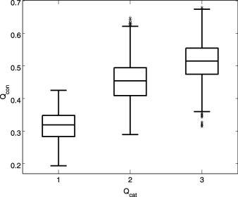
Figure 4: Boxplots showing the distribution of $Q_{\mathrm{con}}$ for each level of $Q_{\mathrm{cat}}=1,2$ and $3$ for DB1.

Analysis and interpretation for the forensic practitioner: We illustrate how PRCs can be obtained for a pair of prints under investigation in forensic practice. The pair in Figure 1 has $w=7$ matches with $m_{1}=35$ and $m_{2}=49$, and $Q_{\mathrm{cat}}=2$ and $3$ for the left and right images, respectively. Since these images are from FVC2002 DB2, we base our inference using the results from this database. Corresponding to $w=7$, the mean PRC is $0.6395$ with $99.9\%$ credible interval $[0.6263,0.6523]$. The mean value implies that about $64\%$ of random pairings of impostor fingerprints will have minutia matches of $7$ or more. Thus, there is no evidence to suggest that the pair in Figure 1 is something other than a random match (namely, an impostor pair).

The forensic practitioner can also perform a “what if” analysis. If the quality of the images was good with $Q_{\mathrm{cat}}$ taking value $4$ for both images in the pair, then the PRC is reduced to $0.3112$, which still indicates this is more likely a random pairing. With this analysis, a practitioner can eventually conclude that the pairs in question are very likely a random match even in the best case scenario where the image qualities are perfect.

The GLMM procedure can also be utilized to provide a guideline for choices of $w$ that will give desired PRC values for forensic testimony, for example, $\operatorname{PRC}=0.01$ means that the error we make in declaring a positive match when in fact it is not is at most $0.01$. Table 11 provides the smallest values for $w$ for guaranteeing $\operatorname{PRC}(w|m_{1},m_{2})\leq 0.01$ for different $Q_{\mathrm{cat}}$ combinations when $m_{1}=35$ and $m_{2}=49$ based on DB2 with maximum possible number of matches $w$ being ${\operatorname{min}}(m_{1},m_{2})=35$. Based on the $(2,3)$ [or $(3,2)$] entry of the table, we see that the desired $w$ to make a reliable decision for the above prints in question should be $21$. Thus, $w=7$ is too low for making a reliable positive match decision. The $*$ entries corresponding to the lowest quality combinations indicate that even for the maximum value of $w=35$, the PRC never goes below $0.01$. This again emphasizes that positive identification decisions cannot and should not be made with very low quality images. Corresponding results can be obtained for DB1 and DB3 similarly, and for $Q_{\mathrm{con}}$, and are therefore not presented here.

=200pt $\bolds{Q_{1}/Q_{2}}$ $\bolds{1}$ $\bolds{2}$ $\bolds{3}$ $\bolds{4}$ $1$ $*$ $*$ $33$ $29$ $2$ $*$ $25$ $21$ $18$ $3$ $33$ $21$ $17$ $15$ $4$ $29$ $18$ $15$ $13$

Table 11: Smallest $w$ required for $\operatorname{PRC}(w|35,49)\leq 0.01$ based on $Q_{\mathrm{cat}}$ and DB2. $*$ indicates no such $w$ exists

7 Validation based on simulation

We performed simulation and validation experiments for DB1 and DB2 with $F=100$ fingers and $L=8$ impressions per finger. $Q_{\mathrm{cat}}$ and $Q_{\mathrm{con}}$ levels were fixed as in the respective databases, but the total number of minutia matches $Y_{ij}$ for each pair of prints $(i,j)$ (see Section 3 for the GLMM model and related notation) were simulated from the GLMM model with fixed and known parameter values $\bolds{\tau}=(\bolds{\theta}^{\prime},\operatorname{log}(\sigma^{2}))^{\prime}$. The parameter values were fixed at the estimated values obtained based on real data for DB1 and DB2, as given in Tables 4 and 5. As noted previously, our inference procedure yields posterior mean and standard deviation estimates as well as $99.9\%$ credible intervals as mentioned in Section 4. The coverage probabilities of each credible interval were calculated for all the true parameter values as well as the true PRC values based on $50$ runs. We use the coverage probabilities as a measure of how well the Laplace method approximates the exact GLMM likelihood for large $F$. Based on simulations, we find that the average coverage probabilities for parameters and PRC values (averaged over all three databases) are approximately $98\%$ and $98.5\%$, respectively. There is some underestimation of the coverage probability but not grossly so, indicating that the Laplace approximation to the GLMM likelihood is good even for $F=100$.

8 Summary and discussion

To assess the extent of fingerprint individuality for different image quality of prints, a GLMM framework and Bayesian inference procedure is developed. Our inference scheme is able to provide a point estimate as well as a credible interval for the PRC depending on the image quality and the observed number of matches between a pair of prints. Numerical reports of the PRC are obtained which can be used to validate forensic testimony. Further, we also provide the smallest number of minutia matches $w$ needed to keep the PRC around a prespecified (small) number. These matching numbers serve as a guideline and safeguard against falsely deciding a positive match when the quality of the prints is unreliable. The best report of fingerprint individuality is obtained when both or at least one is of very good quality and the other is of good quality. No inference on individuality should be made when either print is of moderate to poor quality as observed from our experimental results; having poor quality latent prints, for example, severely hampers reliable matching results.

As far as we know, previous work has not considered including image quality in fingerprint individuality assessment in a quantitative manner and in a formal statistical framework. Our work can be used as a baseline in forensic applications for acquiring a quantitative assessment of individuality given two prints in question. Regardless of whether the prints are of poor or good quality, the methodology outlined will output a PRC value. This PRC value could serve as a baseline and as a first guide to what extent there is evidence beyond a reasonable doubt. The subsection of Section 6 titled “Analysis and inference for the forensic practitioner” highlights the kinds of analysis that may be conducted based on the GLMM methodology. The GLMM method still does not utilize other fingerprint features such as type of minutiae detected, ridge lengths and the class of fingerprint, which could potentially further decrease the PRC and increase the extent of individualization. This will be addressed in a future work.

Intra-finger correlations and inter-finger variability: The incorporation of the random effects $b_{f}$ is very important in any statistical analysis involving different fingers and multiple impressions per finger. The random effects $b_{f}$ serve to model both intra-finger correlations as well as inter-finger variability. Models that incorporate correlations due to multiple impressions of the same finger give very different results compared to models that do not account for this. For example, Dass and Jain (2006) show that the upper and lower confidence bounds are misleadingly narrower if correlations, when present, are not taken into account. Similarly, the upper and lower credible bounds for the PRC will be affected if one does not account for intra-finger correlations. The random effects $b_{f}$ also serve another purpose. They model inter-finger variability as we move from different fingers in the target population; the database is merely a representative sample of the target population of fingers for which the true population PRC is unknown and has to be estimated. In Zhu, Dass and Jain (2007), the PRC was calculated for each pair of print based on minutia distributions on the respective fingers. However, this is not a representative PRC for the entire fingerprint database. Thus, Zhu, Dass and Jain (2007) considered clustering the minutia distributions for the entire fingerprint database. A more formal approach for obtaining inference for population level PRCs was addressed in Dass and Li (2009). The random effects $b_{f}$ in the present context represent deviations in the target population, thus enabling inference for this overall population PRC to be made.

Alignment of prints: The alignment prior to matching a pair of prints is not a separate issue but a function of the detected minutia. Based on the detected minutia in a print, the alignment with the other print is done by first aligning a pair of detected minutiae (one from each print), then finding the optimal translation (via the paired minutiae locations) and rotation (via the paired minutiae directions) that exactly aligns the two. So, one can see that the alignment is also a function of image quality: For poor quality images, more spurious minutiae are detected and, hence, the alignment can be more random (compared to the true alignment based on genuine minutia). The randomness in the alignment also contributes to increasing the number of minutia matches, $Y_{ij}$, for poor quality images. We do not model the alignment separately because of the fact that its randomness, which depends on spurious minutia, is captured in the observed $Y_{ij}$.

Fusion schemes: The difference in the estimates of fingerprint individuality for the three databases can be attributed to the intrinsic nature of the images in these separate databases. For the databases considered, the intrinsic variability arises due to the different sensors used, the extent of distortion due to varying skin elasticity and the composition of the subjects (manual workers versus aged population and others). Where forensic application is concerned, it is usually the practice to match a latent print to template prints in a database. The sensor used to acquire the templates is known and, therefore, it makes sense to report sensor-specific estimates of fingerprint individuality. However, sensor-specific estimates should not be too different from each other: A significant difference in the reported PRCs (using sensor-specific models) indicates systematic bias of that particular sensor toward or against random matching. As we mentioned and observed earlier, we also find significant variability (as well as overlap) in $Q_{\mathrm{con}}$ values corresponding to different $Q_{\mathrm{cat}}$ levels. This motivates us to consider GLMMs and inference for PRCs based on combining two or more quality covariates that measure different aspects of image clarity. It is possible to arrive at a single measure of fingerprint individuality by incorporating additional random effects (for different fingerprint databases and sensors) and fixed effects (for two or more quality measures) in the GLMM formulation. We will investigate these fusion issues in our future research.

References

- Dass (2010) {barticle}[auto:STB—2014/02/12—14:17:21] \bauthor\bsnmDass, \bfnmS.\binitsS. (\byear2010). \btitleAssessing fingerprint individuality in presence of noisy minutiae. \bjournalIEEE Trans. of Information Forensics and Security \bvolume5 \bpages62–70. \bptokimsref\endbibitem
- Dass and Jain (2006) {barticle}[auto:STB—2014/02/12—14:17:21] \bauthor\bsnmDass, \bfnmS.\binitsS. and \bauthor\bsnmJain, \bfnmA. K.\binitsA. K. (\byear2006). \btitleValidating a biometric authentication system: Sample size requirements. \bjournalIEEE Transactions on Pattern Analysis and Machine Intelligence \bvolume28 \bpages1902–1319. \bptokimsref\endbibitem
- Dass and Li (2009) {barticle}[auto:STB—2014/02/12—14:17:21] \bauthor\bsnmDass, \bfnmS.\binitsS. and \bauthor\bsnmLi, \bfnmM.\binitsM. (\byear2009). \btitleHierarchical mixture models for assessing fingerprint individuality. \bjournalAnn. Appl. Stat. \bvolume3 \bpages1448–1466. \bidmr=2752141 \bptokimsref\endbibitem
- Dass, Lim and Maiti (2014) {bmisc}[author] \bauthor\bsnmDass, \binitsS. C., \bauthor\bsnmLim, \binitsC. and \bauthor\bsnmMaiti, \binitsT. (\byear2014). \bhowpublishedSupplement to “A generalized mixed model framework for assessing fingerprint individuality in presence of varying image quality.” DOI:\doiurl10.1214/14-AOAS734SUPP. \bptokimsref \endbibitem
- Daubert vs. Merrell Dow Pharmaceuticals (1995) {bmisc}[auto:STB—2014/02/12—14:17:21] \borganizationDaubert vs. Merrell Dow Pharmaceuticals (\byear1995). \bhowpublished509 U.S. 579, 113 S. Ct. 2786, 125 L.Ed.2d 469. \bptokimsref\endbibitem
- FVC2006 (2006) {bmisc}[auto:STB—2014/02/12—14:17:21] \borganizationFVC2006: Fingerprint Verification Competition (\byear2006). \bhowpublishedhttp://bias.csr.unibo.it/fvc2006/. \bptokimsref\endbibitem
- Home Office Automatic Fingerprint Recognition System (HOAFRS), License 16-93-0026 (1993) {bmisc}[auto:STB—2014/02/12—14:17:21] \borganizationHome Office Automatic Fingerprint Recognition System (HOAFRS), License 16-93-0026 (\byear1993). \bhowpublishedScience and technology group. Home Office, London. \bptokimsref\endbibitem
- Lehmann and Romano (2005) {bbook}[mr] \bauthor\bsnmLehmann, \bfnmE. L.\binitsE. L. and \bauthor\bsnmRomano, \bfnmJoseph P.\binitsJ. P. (\byear2005). \btitleTesting Statistical Hypotheses, \bedition3rd ed. \bpublisherSpringer, \blocationNew York. \bidmr=2135927 \bptokimsref\endbibitem
- Maio et al. (2002) {bincollection}[auto:STB—2014/02/12—14:17:21] \bauthor\bsnmMaio, \bfnmD.\binitsD., \bauthor\bsnmMaltoni, \bfnmD.\binitsD., \bauthor\bsnmCappelli, \bfnmR.\binitsR., \bauthor\bsnmWayman, \bfnmJ. L.\binitsJ. L. and \bauthor\bsnmJain, \bfnmAnil K.\binitsA. K. (\byear2002). \btitleFVC2002: Fingerprint verification competition. In \bbooktitleProceedings of the International Conference on Pattern Recognition (ICPR) \bpages744–747. \bpublisherIEEE Computer Society, \blocationQuebec, Canada. \bptokimsref\endbibitem
- National Academy of Sciences Committee on Identifying the Needs of the Forensic Science Community, National Research Council (2009) {bmisc}[auto:STB—2014/02/12—14:17:21] \borganizationNational Academy of Sciences Committee on Identifying the Needs of the Forensic Science Community, National Research Council (\byear2009). \bhowpublishedStrengthening forensic science in the United States: A path forward. National Academies Press. \bptokimsref\endbibitem
- Pankanti, Prabhakar and Jain (2002) {barticle}[auto:STB—2014/02/12—14:17:21] \bauthor\bsnmPankanti, \bfnmS.\binitsS., \bauthor\bsnmPrabhakar, \bfnmS.\binitsS. and \bauthor\bsnmJain, \bfnmA. K.\binitsA. K. (\byear2002). \btitleOn the individuality of fingerprints. \bjournalIEEE Transactions on Pattern Analysis and Machine Intelligence \bvolume24 \bpages1010–1025. \bptokimsref\endbibitem
- Shun and McCullagh (1995) {barticle}[mr] \bauthor\bsnmShun, \bfnmZhenming\binitsZ. and \bauthor\bsnmMcCullagh, \bfnmPeter\binitsP. (\byear1995). \btitleLaplace approximation of high-dimensional integrals. \bjournalJ. Roy. Statist. Soc. Ser. B \bvolume57 \bpages749–760. \bidissn=0035-9246, mr=1354079 \bptokimsref\endbibitem
- Tabassi, Wilson and Watson (2004) {bmisc}[auto:STB—2014/02/12—14:17:21] \bauthor\bsnmTabassi, \bfnmE.\binitsE., \bauthor\bsnmWilson, \bfnmC.\binitsC. and \bauthor\bsnmWatson, \bfnmC.\binitsC. (\byear2004). \bhowpublishedFingerprint image quality. Technical Report 7151. Available at http://fingerprint.nist.gov/NBIS. \bptokimsref\endbibitem
- U.S. vs. Byron C. Mitchell (1999) {bmisc}[auto:STB—2014/02/12—14:17:21] \borganizationU.S. vs. Byron C. Mitchell (\byear1999). \bhowpublishedCriminal Action No. 96-407, U.S. District Court for the Eastern District of Pennsylvania. \bptokimsref\endbibitem
- Zhu, Dass and Jain (2007) {barticle}[auto:STB—2014/02/12—14:17:21] \bauthor\bsnmZhu, \bfnmY.\binitsY., \bauthor\bsnmDass, \bfnmS. C.\binitsS. C. and \bauthor\bsnmJain, \bfnmA. K.\binitsA. K. (\byear2007). \btitleStatistical models for assessing the individuality of fingerprints. \bjournalIEEE Transactions on Information Forensics and Security \bvolume2 \bpages391–401. \bptokimsref\endbibitem