Why is the electrocaloric effect so small in ferroelectrics?

Abstract

Ferroelectrics are attractive candidate materials for environmentally friendly solid state refrigeration free of greenhouse gases. Their thermal response upon variations of external electric fields is largest in the vicinity of their phase transitions, which may occur near room temperature. The magnitude of the effect, however, is too small for useful cooling applications even when they are driven close to dielectric breakdown. Insight from microscopic theory is therefore needed to characterize materials and provide guiding principles to search for new ones with enhanced electrocaloric performance. Here, we derive from well-known microscopic models of ferroelectricity meaningful figures of merit for a wide class of ferroelectric materials. Such figures of merit provide insight into the relation between the strength of the effect and the characteristic interactions of ferroelectrics such as dipolar forces. We find that the long range nature of these interactions results in a small effect. A strategy is proposed to make it larger by shortening the correlation lengths of fluctuations of polarization. In addition, we bring into question other widely used but empirical figures of merit and facilitate understanding of the recently observed secondary broad peak in the electrocalorics of relaxor ferroelectrics.

The thermal changes that occur in ferroelectric (FE) materials upon the application or removal of electric fields are known as the electrocaloric effect (ECE). Crossley2015a ; Moya2014a ; Alpay2014a ; Correia2014a ; Valant2012a ; Scott2011a ; Guo2009a The effect was first studied in Rochelle salt in 1930 Kobeko1930a and it’s the electric analogue of the magnetocaloric effect, which is commonly used to reach temperatures in the milliKelvin range. The ECE is the result of entropy variations with polarization, e.g., isothermal polarization of a ferroelectric reduces its entropy while depolarization increases it. It is parametrized by isothermal changes in entropy $\Delta S$ and adiabatic changes in temperature $\Delta T$ and it is strongest near the ferroelectric transition.

Since the phase transitions occur near room temperature in many FEs, the potential for using the ECE for cooling applications is huge: it could provide an alternative to standard refrigeration technologies based on the vapor-compression method in which the running substances are greenhouse gases such as freon and hydrochlorofluorocarbons; Narayan2012a replace the widely used but inefficient small thermoelectric cooling devices such as Peltier coolers; Moya2014a and lead to energy harvesting applications. Sebald2014a Moreover, developing cooling prototypes based on the ECE Narayan2009a ; Jia2012a ; Gu2013a may have several advantages over those based on the more studied magnetocaloric effect as the magnetic materials of interest require expensive rare-earth elements and large magnetic fields, while many FEs are ceramics or polymers, which are cheap and can be driven with electric fields that are easy to generate.

Though promising, a major challenge is that the magnitude of the ECE remains too small for useful applications: in bulk FEs, $\Delta T$ is usually less than a few milliKelvin per Volt and $\Delta S$ is usually a fraction of a JK^-1mol^-1. Moya2014a FE thin films exhibit ECEs of about an order of magnitude larger than their bulk counterparts as they can withstand larger breakdown electric fields. Mischenko2006a Thin films, however, have small cooling power because of their small heat capacities. Ferroelectric polymers have also received considerable attention with ECEs comparable to those of thin films, though they must be driven at larger electric fields than those of thin films. Neese2008a

In the light of these challenges, it has been recently pointed out that insight from microscopic theory into the ECE may contribute to characterize known materials and provide guiding principles to search for new ones with enhanced electrocaloric performance. Moya2014a Here, we provide such insight by deriving meaningful figures of merit from well-known microscopic models of ferroelectricity. Our figure of merit allow us to set trends across different classes of FE materials (order-disorder and displacive) and provides insight into the relation between the magnitude of the ECE and the characteristic interactions of FEs (e.g. dipolar and strain). We find that the long-range nature of these interactions produces trade-offs in the ECE: while they can give rise to high transition temperatures (i.e., comparable to room temperature), they concomitantly give rise to long correlation lengths of polarization at finite electric fields, which, as we show here, result in a small effect. We make contact with well-known results derived from Landau theory Lines1977a and those from heuristic arguments. Pirc2011b Based on these findings, we then study the effects of compositional disorder. The purpose of this is twofold: to propose a strategy to increase the magnitude of the ECE and to model the ECE of so-called relaxor ferroelectrics - a widely studied class of electrocaloric materials with diffuse phase transitions that could provide a broad temperature range of operation in a cooling device. Pirc2011b ; Shebanov1992a ; Mischenko2006b ; Hagberg2008a ; Correia2009a ; Lu2010a ; Valant2010a ; Dunne2011a ; Rozic2011a ; Pirc2011a ; Goupil2012a ; Perantie2013a ; LeGoupil2014a We find that the commonly observed secondary broad peak in the ECE of relaxors Hagberg2008a ; Perantie2013a is expected in any ferroelectric that is deep in the supercritical region of their phase diagram. Our results also bring into question the common practice of defining the electrocaloric strength of a material as the ratio of the entropy or temperature changes over the change in applied electric field. Moya2014a ; Valant2012a

To illustrate the ideas presented above, we adhere to a simple microscopic model for displacive ferroelectrics with quenched random electric fields. Guzman2013a Such compositional disorder is typical of relaxor ferroelectrics such as the prototype PbMg_1/3Nb_2/3O₃ (PMN) and it arises from the different charge valencies and disordered location of the Mg²⁺ and Nb⁵⁺ ions. In the absence of disorder, it is a standard minimal model of ferroelectricity. Lines1977a With disorder, the model gives a good starting point for the description of the static dielectric properties of relaxors. Guzman2013a ; Guzman2015a

In calculating the ECE in the presence of compositional disorder, it is important to recall that Maxwell relations are not applicable. Maxwell relations are usually invoked in ferroelectrics to indirectly determine, for instance, adiabatic changes in temperature $\Delta T$ from the variations of the polarization with respect to temperature. Valant2012a Pure ferroelectrics are in thermodynamic equilibrium, thus Maxwell relations hold. Disordered ferroelectrics are not in thermodynamic equilibrium, thus Maxwell’s relations do not apply. This is supported by the recent experimental observation that direct measurements of $\Delta T$ in solutions of the relaxor ferroelectric polymer PVDF-TrFE-CFE with PVDF-CTFE were significantly larger than those estimated from their polarization curves. Lu2010a Another difficulty is that Landau theory fails for relaxors. Landau theory is applicable away from the region of critical fluctuations of polarization that occur near the transition point. In conventional ferroelectrics, Landau theory works remarkably well since this region is narrow. Lines1977a In relaxors, on the other hand, Landau theory is not expected to hold as the region of fluctuations is broad. We overcome both of these difficulties by calculating the ECE directly from the entropy function, as described in the supplementary material (SM). SM

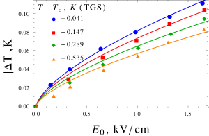
Figure 1: Applied electric field dependence of the adiabatic changes in temperature near the paraelectric-to-ferroelectric transition ($T_{c}^{0}\simeq 322\,$K) in triglycine sulphate (TGS). Solid lines correspond to fits to the electric field to the power of $2/3$ as predicted by Eq. (3). Data taken from Ref. [Strukov1964a, ].

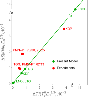
Figure 2: Figures of merit at the paraelectric-to-ferroelectric transition for several ferroelectrics. Axes are in units of (statvolt/cm)^2/3. Here, TSCC = (CH₃NHCH₂COOH)₃CaCl₂, KDP = KH₂PO₄, TGS = (NH₂CH2COOH)₃ $\cdot$ H₂SO₄, LNO = LiNbO₃, LTO = LiTaO₃, and PMN-PT ${1-x}/x$ = (PbMg_1/3Nb_2/3O₃)_1-x-(PbTiO₃)_x. Data taken from Refs. [Moya2014a, , Strukov1964a, , Mackeviciute2013a, ].

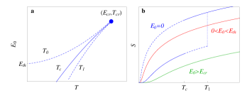
Figure 3: (a) Schematic of the electric field-temperature phase diagram for ferroelectric with disorder. The coexistence line (blue) ends at a critical point $(E_{cr},T_{cr})$. Spinodal curves $T_{0}$ and $T_{1}$ indicate the end of the stability of the paraelectric and ferroelectric states, respectively. (b) Schematic entropy-temperature phase diagram for various electric field regimes. Solid and dashed lines correspond to stable and metastable states, respectively. The entropy function for $E_{th}<E_{0}<E_{tr}$ is not shown for clarity.

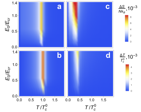
Figure 4: Density plots of the adiabatic changes in temperature and isothermal changes in entropy for (a)-(b) no and (c)-(d) moderate  ($(\Delta^{2}/v_{0})/(k_{B}T_{c}^{0})=2.0\times 10^{-2}$) disorder. As expected, $\Delta S$ and $\Delta T$ in all cases are small except at the onset of the ferroelectric transition. For moderate disorder, $\Delta S$ increases as a result the shortening of the correlation length, while $\Delta T$ decreases as $T_{c}$ shifts to lower temperatures. $v_{0}$ is the zone-center Fourier component of the dipolar force.

We first consider the case without compositional disorder. In the absence of disorder and no applied electric field, the model gives a second-order paraelectric-to-ferroelectric phase transition at a transition temperature $T_{c}^{0}$. Consider an isothermal change in entropy $\Delta S(T,E_{0})$ near $T_{c}^{0}$ that results from a change in electric field $\Delta E_{0}=0\to E_{0}$. Within a mean field approximation, we find that (see SM), SM

$$\frac{|\Delta S(T,E_{0})|}{Nk_{B}}=\frac{3\zeta a^{2}}{8\pi}\left[\xi^{-2}(T,E_{0})-\xi^{-2}(T,0)\right],$$ (1)

where $\zeta$ is a dimensionless coefficient that depends on the lattice structure, $a$ is the lattice constant and $N$ is the number of lattice sites. Guzman2013a $\xi(T,E_{0})$ is the correlation length of the exponentially decaying fluctuations of polarization at the field $E_{0}$ and temperature $T$. Lines1977a It is given by the (soft) frequency of the transverse optic phonon mode Guzman2013a and it diverges as $\xi(0,T)\propto\left(|T-T_{c}|\right)^{-1/2}$ at the onset of the FE transition. Lines1977a A similar relation is derived for the adiabatic changes in temperature $\Delta T(T_{1},E_{0})=T_{2}-T_{1}$ (see SM), SM

$$\frac{\Delta T(T_{1},E_{0})}{T_{1}}=\frac{3\zeta a^{2}}{8\pi}\left[\xi^{-2}(E_{0},T_{2})-\xi^{-2}(0,T_{1})\right].$$ (2)

Equations (1) and (2) relate the ECE to the correlation length of a ferroelectric. We make contact with known results by noting that near the FE transition, $\left(\xi(T,E_{0})/a\right)^{-2}-\left(\xi(T,0)/a\right)^{-2}\simeq(\zeta k_{B}n)^{-1}P_{s}^{2}(T,E_{0})/C_{CW}$ in Eqs. (1), which gives the standard results from Landau theory Lines1977a and similar form to those derived from heuristic arguments. Pirc2011b $P_{s}(T,E_{0})$ is the polarization at temperature $T$ and at field $E_{0}$, $C_{CW}$ is the Curie-Wiess constant, and $n=N/V$ is the number of lattice points per unit volume $V$. At the phase transition, $\Delta S(T_{c}^{0},E_{0})$ and $\Delta T(T_{c}^{0},E_{0})$ of Eqs. (1) and (2) peak as the correlation length at zero field diverges ($\xi(T_{c}^{0},0)=\infty$) and their magnitude depends on that at finite fields. For ferroelectrics, it is well-known that these tend to be large due to the long-range nature of the dipole and strain interactions. Lines1977a

We now derive our figure of merit. By evaluating the correlation length at the critical temperature ($\xi^{-2}(E_{0},T_{c}^{0})\propto\left(T_{c}^{0}/C_{CW}\right)^{1/3}\left(E_{0}/P_{s}^{0}\right)^{2/3}$) in Eqs. (1) and (2), we obtain the magnitude of the ECE in terms of dielectric properties of a FE (see SM), SM

$$\frac{\Delta T(T_{c}^{0})}{T_{c}^{0}}\simeq\frac{\Delta S(T_{c}^{0})}{Nk_{B}}\propto\left(\frac{T_{c}^{0}}{C_{CW}}\right)^{1/3}\left(\frac{E_{0}}{P_{s}^{0}}\right)^{2/3},$$ (3)

where $P_{s}^{0}=P_{s}(0,0)$ is the saturated polarization at zero field. The coefficient of proportionality is a dimensionless number ($(1/2)(27/(4\pi))^{2/3}\simeq 0.8$). Eq. (3) is our figure of merit. A similar calculation for an order-disorder FE gives a figure of merit similar to that of Eq. (3) with two differerences: the ratio $T_{c}^{0}/C_{CW}$ is fixed to $1/3$ (a well-known result of pure order-disorder models Strukov1998a ) and a constant of proportionality of  ($(1/3)^{1/3}(1/2)(27/(4\pi))^{2/3}\simeq 0.6$).

The available data confirm the non-linearity predicted by our simple model: figure 1 shows that $\Delta T\propto E_{0}^{2/3}$ near the ferroelectric transition of triglycine sulphate (NH₂ CH₂COOH)₃ $\cdot$ H₂ SO₄ ). Similar scaling laws have been observed in the magnetocaloric effect. Franco2010a The non-linearity in $E_{0}$ suggests that it is not meaningful to define $\Delta S/\Delta E_{0}$ or $\Delta T/\Delta E_{0}$ as the electrocaloric strength of an electrocaloric material when $\Delta S$ and $\Delta T$ are measured near or at the transition temperature. Moya2014a ; Valant2012a

From Eq. (3) and data from the literature, Landolt-Bornstein we calculate our figure of merit for several FE materials. The results are shown in Figure 2. Our model predicts a clear trend: order-disorder FEs should display larger ECE than that of the displacive type. This is a consequence of the shorter correlation lengths that the former type generally display compared to those of the latter type (order-disorder Curie-Weiss constants are typically about two orders of magnitude smaller than those of displacive FEs). An exception to this rule may exist, however, in the ultraweak displacive FEs such as tris-sarcosine calcium chloride (TSCC). Our predicted figure of merit is an order of magnitude larger than any of the FEs considered here as a result of their exceptionally small Curie-Weiss constants and spontaneous polarization (which result in shorter correlation lengths). Mackeviciute2013a The ECE has been recently measured in brominated TSCC compounds, however, we cannot compare to our model as the measurement was performed near its quantum critical point. Rowley2015a When Eq. (3) is contrasted to experiments, Moya2014a there are clear discrepancies which we attribute to the mixed order-disorder and displacive character that most FEs display, and to their large anharmonicities (beyond quartic order). These differences, though, are not too severe specially when considering the simplicity of the model.

We now consider the effects of compositional disorder. To do so, we consider the minimal model for relaxor ferroelectrics presented in Refs. [Guzman2013a, ] and [Guzman2015a, ]. Such model includes dipolar interactions and short-range harmonic and anharmonic forces for the critical modes as in the theory of pure ferroelectrics together with quenched disorder coupled linearly to the critical modes. In formulating this model, it is important to recall Onsager’s result Onsager1936a that unlike in the Clausius-Mossotti or Lorentz approximation, dipole interactions alone do not lead to ferroelectic order except at $T=0$. Also that pure ferroelectric transitions were understood with the realization Cochran-Anderson that they are soft transverse optic mode transitions due to dipoles induced by structural transitions so that the low temperature phase does not have a center of symmetry. The first point is not in practice important for pure ferroelectrics which are well described by a mean-field theory for the dielectric constant, and is often a first order transition only below which the dipoles are produced. Lines1977a But as it was shown in Refs. [Guzman2013a, ] and [Guzman2015a, ], in relaxors the random location of defects acts in concert with the dipole interactions to extend the region of fluctuations to zero temperatures. Therefore dipole interactions must be a necessary part of the model. The essential physical points in the simplest necessary solution is to formulate a theory which considers thermal and quantum fluctuations at least at the level of the Onsager approximation Onsager1936a and random field fluctuations at least at the level of a replica theory. The model Hamiltonian and minimal solution are given in the supplementary material. SM

Following Ref. [Guzman2013a, ], we parametrize the quenched random electric fields by a Gaussian probability distribution with zero mean and variance $\Delta^{2}$. SM Figures 3 (a)-(b) show an schematic of the electric field-temperature ($E-T$) phase diagram and the entropy function for moderate disorder. There are metastable paraelectric states with a stability region that extends to zero temperature. Ferroelectric states appear as local minima in the free energy at high temperatures and become stable below a coexistence temperature $T_{c}<T_{c}^{0}$. The coexistence line of the polar and non-polar phases ends at a critical point $(T_{cr},E_{cr})$. Weak first-order phase transitions are induced for electric fields greater than a threshold field $E_{th}$ as they cross the region of stability of the metastable paraelectric phase. For fields smaller than $E_{th}$, no macroscopic ferroelectric transition occurs with a spontaneous polarization. In typical relaxors such as PMN, $E_{th}\simeq 2\,$kV/cm and $(T_{cr},E_{cr})\simeq(240\,\mbox{K},4\,\mbox{kV/cm})$. Kutnjak2007a

Figures 4(a)-(d) show the electric field and temperature dependences of the ECE for zero and moderate disorder. In both cases the peaks in $\Delta S$ and $\Delta T$ occur at their corresponding transition temperatures and increase monotonically with increasing applied field, as expected. For moderate disorder, however, $\Delta S$ increases provided the applied field is greater than $E_{th}$. This increment occurs because of the shortening of the correlation length , as indicated by Eq. (3). Though $\Delta T$ is also affected by the shortening of the correlation length, it decreases with disorder as $T_{c}$ shifts to lower temperatures. We emphasize here that we are referering to the correlation length of fluctuations of polarization and not to the characteristic nanoscaled size of polar domains of relaxors. Shi2011a

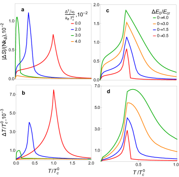
Figure 5: (a)-(b) Calculated dependence of the ECE with compositional disorder for strong changes in the electric field $\Delta E_{0}/E_{cr}=0\to 1.5$. (c)-(d) Calculated ECE of a FE with moderate compositional disorder  ($(\Delta^{2}/v_{0})/(k_{B}T_{c}^{0})=2.0\times 10^{-2}$) for several electric field strengths.

Figures 5 (a)-(b) show $\Delta S$ and $\Delta T$ for several disorder strengths and for a fixed change in the electric field ($\Delta E_{0}>0\to E_{cr}$). The increment in $\Delta S$ from weak-to-moderate disorder is clearly shown here together with the monotonic decrease in $\Delta T$. For strong disorder, the ECE is weak since the dipoles are pinned by the random fields, therefore the entropy does not change significantly upon the application or removal of electric fields. Our model is qualitative and fairly good quantitative agreement with the ECE effect observed in typical relaxors where direct temperature measurements in PMN-PT show that a sharp peak in $\Delta T$ shifts to higher temperatures and increases its magnitude with increasing PT concentration (up to the morphotropic phase boundary). Perantie2013a

Figures 5 (c)-(d) show $\Delta S$ and $\Delta T$ for several electric field strengths and for fixed (moderate) disorder. As the electric field changes increase, a broad peak develops in addition to the usual sharp one at $T_{c}$. Such broad peak in $\Delta T$ is commonly observed in relaxors and it is usually attributed to nanoscaled polar domains. Dunne2011a ; Perantie2013a However, our model predicts a broad peak occurs in $\Delta T$ already in the absence of compositional disorder (where there are no polar nanodomains) for very strong fields. Therefore, the broad peak is simply the expected maximum in the ECE for a ferroelectric that is deep in the supercritical regime, i.e., away from the critical point ($(T,E_{0})\gg(T_{cr},E_{cr})$). We obtain similar results from Landau theory. SI Experimentally, this broad peak is not observed in conventional ferroelectrics as their breakdown fields are close to their critical fields, e.g., $E_{cr}\simeq 10\,$kV/cm Novak2013a and $E_{breakdown}\simeq 14\,$kV/cm Landolt-Bornstein for BaTiO₃.

Starting from well-known microscopic models of ferroelectricity, we have derived a meaningful figure of merit for the ECE in a wide class of FE materials. When defining a figure of merit for a caloric effect, we find crucial to account for the well-known non-linearities that occur near the FE transition. The large correlation lengths of fluctuations of polarization of FEs, result in a small ECE. We predict that ultraweak FEs such as those of the TSCC-family should exhibit figures of merit of about an order of magnitude larger than those of conventional displacive and order-disorder FEs. Shortening the correlation lengths results in larger isothermal changes in entropy, lower transition temperatures, and smaller adiabatic changes in temperature. Broad peaks in the ECE such as those that have been observed in relaxors are expected for any ferroelectric that can go well into the supercritical region. Our work has implications beyond the ECE as a similar analysis could be performed for other caloric effects such as magneto- and mechano-caloric effects, which are currently being studied extensively. Moya2014a Our results in combination with other recently proposed figures of merit Defay2013a ; Moya2015a should provide guidance for characterizing known caloric materials and designing new ones with enhanced performance.

Acknowledgements. We acknowledge useful discussions with Neil Mathur, Sohini Kar-Narayan, Xavier Moya, Karl Sandeman, and Chandra Varma. We thank James Scott for his comments and suggestions on the manuscript. Work at Argonne is supported by the U.S. Department of Energy, Office of Basic Energy Sciences under contract no. DE-AC02-06CH11357.

Supplemental Material: - Why is the electrocaloric effect so small in ferroelectrics?

I Microscopic Model

In this section we present the microscopic model from which we calculate the ECE. The model was recently proposed in Ref. [Guzman2013a, ] for relaxor ferroelectrics. We present it here for the sake of completeness. We focus on the relevant transverse optic mode configuration coordinate $u_{i}$ of the ions in the unit cell $i$ along the polar axis (chosen to be the $z$-axis). $u_{i}$ experiences a local random field $h_{i}$ with probability $P(h_{1},h_{2},...)$ due to the compositional disorder introduced by the different ionic radii and different valencies of, say, Mg²⁺, Nb⁵⁺, and Ti⁴⁺ in the typical relaxor (PMN)_1-x-(PT)_x. The model Hamiltonian is

$$H=\sum_{i}\left[\frac{\Pi_{i}^{2}}{2M}+V(u_{i})\right]-\frac{1}{2}\sum_{i,j}v_{ij}u_{i}u_{j}-\sum_{i}h_{i}u_{i}-E_{0}\sum_{i}u_{i}$$ (S1)

where $\Pi_{i}$ is the momentum conjugate to $u_{i}$, $M$ is an effective mass, and $E_{0}$ is a static applied electric field. We assume the $h_{i}$’s are independent random variables with Gaussian probability distribution with zero mean and variance $\Delta^{2}$. $V(u_{i})=\frac{\kappa}{2}u_{i}^{2}+\frac{\gamma}{4}u_{i}^{4}$ is an anharmonic potential with $\kappa,~{}\gamma$ positive constants. $v_{ij}/{e^{*}}^{2}=\begin{cases}3\frac{(Z_{i}-Z_{j})^{2}}{|{\bm{R}}_{i}-{\bm{R}}_{j}|^{5}}-\frac{1}{|{\bm{R}}_{i}-{\bm{R}}_{j}|^{3}},&{\bm{R}}_{i}\neq{\bm{R}}_{j}\\ 0,&{\bm{R}}_{i}={\bm{R}}_{j},\end{cases}$ is the dipole interaction where $e^{*}$ is the effective charge and $Z_{i}$ is the $z$-component of ${\bm{R}}_{i}$. For future use, we denote $v_{\bm{q}}=\sum_{i,j}v_{ij}e^{i{\bm{q}}\cdot({\bm{R}}_{i}-{\bm{R}}_{j})}$ the Fourier transform of the dipole interaction, $v_{0}~{}(=4\pi n{z^{*}}^{2}/3)$ the ${\bm{q}}\to 0$ component of $v_{\bm{q}}$ in the direction transverse to the polar axis $\hat{\bm{z}}$ ($v_{\bm{q}}$ is non-analytic for ${\bm{q}}\to 0$), $n$ the number of unit cells per unit volume, and $a$ the lattice constant.

II Variational Solution and Entropy Function

In the present section, we briefly describe the variational solution of the problem posed by the Hamiltonian (S1) and obtain an expression for the entropy function.

We consider a trial probability distribution, $\rho^{tr}=e^{-\beta H^{tr}}/Z^{tr}$ where $H^{tr}=\sum_{i}\frac{\Pi_{i}^{2}}{2M}+\frac{1}{2}\sum_{i,j}(u_{i}-p)G_{i-j}(u_{j}-p)-\sum_{i}h_{i}u_{i},$ is the Hamiltonian of coupled displaced harmonic oscillators in a quenched random field, and $Z^{tr}=\mbox{Tr}e^{-\beta H^{tr}}$ its normalization. where $\Pi_{i}$ is the conjugate momentum of the displacement coordinate $u_{i}$ at site $i$ and $M$ is an effective mass.

We consider random fields $\{h_{1},h_{2},\dots\}$ with Gaussian probability distribution $P(h_{1},h_{2},...)$ with zero mean and variance $\Delta^{2}$. $p$ is an uniform order parameter: it is the displacement coordinate averaged over thermal disorder first, and then over compositional disorder, $p=\int_{-\infty}^{\infty}dh_{1}dh_{2}\cdots P(h_{1},h_{2},...)\,\mbox{Tr}\,\rho^{tr}\,u_{i}$; $\Omega_{\bm{q}}$ is the frequency of the transverse optic mode at wavevector ${\bm{q}}$ and it is given by the Fourier transform of $G_{i-j}$, $M\Omega_{\bm{q}}^{2}=\sum_{i,j}G_{i-j}e^{i{\bm{q}}\cdot({\bm{R}}_{i}-{\bm{R}}_{j})}$. We define $G_{i-j}^{-1}=\left(1/N\right)\sum_{\bm{q}}(M\Omega_{\bm{q}}^{2})^{-1}e^{-i{\bm{q}}\cdot({\bm{R}}_{i}-{\bm{R}}_{j})}$. $p$ and $\Omega_{\bm{q}}$ are variational parameters and are determined by minimization of the free energy $F=\int_{-\infty}^{\infty}dh_{1}dh_{2}\cdots P(h_{1},h_{2},...)\,\mbox{Tr}\,\rho^{tr}\left[H+k_{B}T\ln\rho^{tr}\right]$.

The entropy $S$ is given as follows,

$$\frac{S}{N} =\int_{-\infty}^{\infty}dh_{1}dh_{2}\cdots P(h_{1},h_{2},...)\,\mbox{Tr}\,\rho^{tr}\,\left(-k_{B}\ln\rho^{tr}\right)$$

$$~{}~{}~{}~{}~{}~{}~{}~{}~{}~{}~{}~{}~{}~{}~{}~{}~{}~{}~{}~{}~{}~{}~{}~{}~{}=\frac{k_{B}}{N}\sum_{\bm{q}}\left\{\frac{\beta\hbar\Omega_{\bm{q}}}{2}\coth\left(\frac{\beta\hbar\Omega_{\bm{q}}}{2}\right)-\ln\left[2\sinh\left(\frac{\beta\hbar\Omega_{\bm{q}}}{2}\right)\right]\right\}.$$ (S2)

$S$ depends on temperature $T=(k_{B}\beta)^{-1}$, the applied static field $E_{0}$; and the stength of compositional disorder $\Delta$. The adiabatic changes in temperature $\Delta T$ and isothermal changes in entropy $\Delta S$ presented in the main text are calculated from Eq. (II). The correlation length of the fluctuations of polarization, $\xi$, is given by the frequency of the transverse optic phonon at the zone center, $\xi/a=\sqrt{(3/4\pi)\zeta/(M\Omega_{0}^{2})}$. SGuzman2013a

III Broad Peak in the ECE of Conventional Ferroelectrics

In this section, we show that Landau theory predicts a broad peak in the ECE of conventional ferroelectrics. We consider the simple Landau theory of Ref. [SNovak2013a, ] for the conventional ferroelectric BaTiO₃ (BTO) in an applied field $E_{0}$ along the $(001)$ axis. Near the the paraelectric-to-ferroelectric transition of BTO, the Landau free energy is given as follows, SNovak2013a

$$F=\frac{a(T-T_{0})}{2}P^{2}+\frac{b}{4}P^{4}+\frac{c}{6}P^{6}+\frac{d}{8}P^{8}-PE,$$ (S3)

where $P$ is the polarization and $T_{0}\simeq 400\,$K is the supercooling temperature. The coefficients $a=1.696\times 10^{6}\,$ Nm²C^-2, $b=3.422\times 10^{9}\,$Nm⁶C^-4, $c=1.797\times 10^{11}\,$Nm¹⁰C^-6, $d=3.214\times 10^{12}\,$Nm¹⁴C^-8 are determined from the dielectric susceptibility and heat capacity experiments. Novak2013a The isothermal changes in temperature $\Delta T=T_{2}-T_{1}$, are calculated self-consistently from the relation $T_{2}=T_{1}\mbox{exp}\left[(a/2C)\left(P^{2}(E_{2},T_{2})-P^{2}(E_{1},T_{1})\right)\right]$, where the temperature and electric field dependence of $P$ are determined by the standard minimization procedure of the free energy (S3). $C$ is the contribution from the lattice to the specific heat.

In the electric field-temperature phase diagram of BTO the spinodal line begins at about $(E_{0},T_{c}^{0})\simeq(0,405\,\mbox{K})$ and ends at a critical point $(E_{cr},T_{cr})\simeq(10\,\mbox{kV/cm},415\,\mbox{K})$. SNovak2013a The paraelectric-to-ferroelectric transition is discontinous along the spinodal line and it is continous at $(E_{cr},T_{cr})$. BTO is supercritical above the critical point and no transition occurs.

Figure S1 (a) shows the adiabatic changes in temperature $\Delta T$ for BTO for several changes in the field strength, $\Delta E_{0}$. $\Delta T$ exhibits a single peak at the transition point for ($\Delta E_{0}\lesssim 0\to 100E_{cr}$), as expected. For larger $\Delta E_{0}$’s than this, a broad peak develops. Clearly, this peak cannot be observed experimentally as the required fields are well beyond BTO’s breakdown electric field ($\simeq 14\,$kV/cm). SLandolt-Bornstein

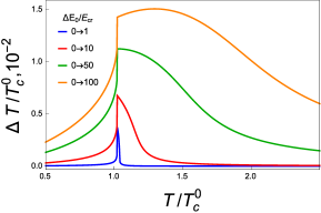
Figure S1: Adiabatic changes in temperature, $\Delta T$ in the conventional ferroelectric BTO for several changes in the electric field strength $\Delta E_{0}$ applied along the $(001)$ direction. A secondary, broad peak arises in $\Delta T$ in addition to that at the transition temperature for very large $\Delta E_{0}$.

IV Figure of Merit

The purpose of this section is to derive our figure of merit given in Eq. (3) of our manuscript. To do so we first derive the relation between the ECE and the correlation length of fluctuations of polarization (Eqs. (1) and (2) of the main text).

We consider the case of no compositional disorder where a mean field approximation is appropriate, as discussed in the main text. In the mean field approximation, the free energy per site $F/N$ of the Hamtilonian (S1) is given as follows, SBlinc1974a

$$\frac{F}{N}=\frac{\kappa}{2}\left(p^{2}+\sigma\right)+\frac{\gamma}{4}\left(p^{4}+6p^{2}\sigma+3\sigma^{2}\right)-\frac{1}{2}v_{0}p^{2}-E_{0}p-\frac{k_{B}T}{2}-k_{B}T\log\left[2\pi\sqrt{M\sigma k_{B}T}\right].$$ (S4)

Here, $p=\left<u_{i}\right>$ is a homogenous order parameter and $\sigma=\left<(u_{i}-\left<u_{i}\right>)^{2}\right>$ are mean squared fluctuations. Minimization of the free energy with respect to $p$ and $\sigma$ gives the following result,

$$E_{0} =\left(M\Omega_{0}^{2}-2\gamma p^{2}\right)p,$$ (S5)

$$M\Omega_{0}^{2} =\kappa+3\gamma\left[\sigma+p^{2}\right]-v_{0},$$ (S6)

$$\sigma =\frac{k_{B}T}{M\Omega_{0}^{2}+v_{0}}.$$ (S7)

Here, $\Omega_{0}$ is the frequency of the zone-center soft mode. Equations (S5)-(S7) are self-consistent equations that determine the temperature and electric field dependence of $\Omega_{0}$ and $p$.

Equations (S5)-(S7) give a second order phase transition at the critical temperature $T_{c}^{0}=\left(v_{0}-\kappa\right)v_{0}^{\perp}/(3\gamma k_{B})$ with a soft mode frequency that follow the Cochran law, $M\Omega_{0}^{2}=3v_{0}(T-T_{c})/C_{CW}$ above about $T_{c}^{0}$ in the absence of an applied field. $C_{CW}=\left(2v_{0}^{\perp}-\kappa\right)v_{0}^{\perp}/(3\gamma k_{B})$ is the Curie-Weiss constant.

The soft mode frequency determines the correlation length of fluctuations of polarization, $\xi$, SGuzman2013a

$$\frac{\xi}{a}=\sqrt{\frac{3\zeta v_{0}/(4\pi)}{M\Omega_{0}^{2}}},$$ (S8)

where $a$ is the lattice constant and $\zeta$ is a dimensionaless constant.

The entropy is given as follows, $S(T,E_{0})=-\left(\partial F/\partial T\right)_{p,\sigma,N}=Nk_{B}\left(1+\ln\sqrt{\sigma T}\right)+$ terms independent of $p,\sigma$ and $T$. Near the FE transition and for weak fields ($M\Omega_{0}^{2}/v_{0}\ll 1$), the entropy is given as follows,

$$\frac{S(T,E_{0})}{Nk_{B}}=\ln T-\frac{1}{2}\frac{M\Omega_{0}^{2}(T,E_{0})}{v_{0}},$$ (S9)

where we have ignored terms independent of $T$. By substituting Eq. (S8) into the above equation and considering changes in the electric field $\Delta E=E_{2}-E_{1}$, we obtain the following result for the magnitude of the isothermal changes in entropy,

$$\frac{\left|\Delta S(T,E_{2},E_{1})\right|}{Nk_{B}}=\frac{3\zeta a^{2}}{8\pi}\left[\xi^{-2}(T,E_{2})-\xi^{-2}(T,E_{1})\right].$$ (S10)

This is our desidered result and corresponds to Eq. (1) in the paper.

We now calculate the adiabatic changes in temperature. For adiabatic processes, Eq. (S9) gives

$$\frac{\Delta T(T_{1},E_{2},E_{1})}{T_{1}}=\frac{3\zeta a^{2}}{8\pi}\left[\xi^{-2}(T_{2},E_{2})-\xi^{-2}(T_{1},E_{1})\right].$$ (S11)

where $\Delta T=T_{2}-T_{1}$ and we have made the assumption that the changes in temperature are small ($\frac{\Delta T}{T_{1}}\ll 1$). This corresponds to Eq. (2) in the main paper.

To derive our figure of merit, we evaluate Eqs. (S10) and (S11) at the transition temperature for $E_{2}=E_{0}>0$ and $E_{1}=0$. From Eqs.  (S5)-(S8) one can show that at $T_{c}^{0}$,

$$\frac{\xi^{-2}(T_{c}^{0},E_{0})}{a^{-2}} =\frac{4\pi v_{0}}{\zeta k_{B}C_{CW}}p^{2}(T_{c}^{0},E_{0}),$$ (S12)

where $p(T_{c}^{0},E_{0})=\left(k_{B}C_{CW}E_{0}/v_{0}^{2}\right)^{1/3}$. The saturated polarization $P_{s}=ne^{*}p(T=0,E_{0}=0)$ is also derived from Eqs. (S5)-(S7) and the result is $P_{s}=\sqrt{9k_{B}nT_{c}^{0}/(4\pi)}$. By substituting all these results into Eq. (S10) we obtain,

$$\frac{\left|\Delta S(T_{c}^{0},E_{0})\right|}{Nk_{B}}=\frac{1}{2}\left(\frac{27}{4\pi}\right)^{2/3}\left(\frac{T_{c}^{0}}{C_{CW}}\right)^{1/3}\left(\frac{E_{0}}{P_{s}^{0}}\right)^{2/3},$$

where we have done the rescaling $E_{0}\to E_{0}e^{*}$ so that $E_{0}$ in the above equation has units of electric field (see Hamiltonian). The same result is obtained for $\Delta T(T_{c}^{0},E_{0})/T_{c}^{0}$. This is our figure of merit given in Eq. (3) of the main text.

References

- (1) S. Crossley, N. D. Mathur, X. Moya, AIP Advances 5, 067153 (2015).
- (2) X. Moya, S. Kar-Narayan, and N. D. Mathur, Nat. Mater. 13, 439 (2014).
- (3) S. Pamir Alpay, J. Mantese, S. Trolier-McKinstry, Q. Zhang, and R. W. Whatmore, MRS Bulletin 39, 1099 (2014).
- (4) T. Correia and Q. Zhang (eds.), Electrocaloric Materials: New generation of coolers (Springer-Verlag, Berlin, 2014).
- (5) M. Valant, Prog. Mater. Sci. 57, 980 (2012).
- (6) J. Scott, Annu. Rev. Mater. Res. 41, 229 (2011).
- (7) S. G. Lu and Q. M. Zhang, Adv. Mater. 21, 1983 (2009).
- (8) P. Kobeko and I. Kurchatov, Z. Phys. 66, 192 (1930).
- (9) S. Kar-Narayan and N. D. Mathur, Ferroelectrics 433, 107 (2012).
- (10) G. Sebald, S. Pruvost, and D. Guyomar, in Electrocaloric Materials: New generation of coolers, edited by T. Correia and Q. Zhang (Springer-Verlag, Berlin, 2014).
- (11) S. Kar-Narayan and N. D. Mathur, Appl. Phys. Lett. 95, 242903 (2009).
- (12) Y. Jia and Y. S. Ju, Appl. Phys. Lett. 100, 242901 (2012).
- (13) H. Gu, X. Qian, X. Li, B. Craven, W. Zhu, A. Cheng, S. C. Yao, and Q. M. Zhang, Appl. Phys. Lett. 102, 122904 (2013).
- (14) A. S. Mischenko, Q. Zhang, J. F. Scott, R. W. Whatmore, and N. D. Mathur, Science 311, 1270 (2006).
- (15) B. Neese, B. Chu, S-G. Lu, Yong Wang, E. Furman, Q. M. Zhang, Science 321, 821 (2008).
- (16) M. E. Lines and A. M. Glass, Principles and Applications of Ferroelectrics and Related Materials (Clarendon Press, Oxford, 1977).
- (17) R. Pirc, Z. Kutnjak, R. Blinc, and Q. M. Zhang J. Appl. Phys. 98, 021909 (2011).
- (18) L. Shebanov and K. Borman, Ferroelectrics 127, 143 (1992).
- (19) A. S. Mischenko, Q. Zhang, R. W. Whatmore, J. F. Scott, and N. D. Mathur, Appl. Phys. Lett. 89, 242912 (2006).
- (20) J. Hagberg, A. Uusimäki, and H. Jantunen, Appl. Phys. Lett. 92, 132909 (2008).
- (21) T. M. Correia, J. S. Young, R. W. Whatmore, J. F. Scott, N. D. Mathur, and Q. Zhang, Appl. Phys. Lett. 95, 182904 (2009).
- (22) S. G. Lu, B. Rožič, Q. M. Zhang, Z. Kutnjak, R. Pirc, Minren Lin, Xinyu Li, and Lee Gorny, Appl. Phys. Lett., 97, 202901 (2010).
- (23) M. Valant, Lawrence J. Dunne, Anna-Karin Axelsson, N. McN. Alford, G. Manos, J. Peräntie, J. Hagberg, H. Jantunen, and A. Dabkowski, Phys. Rev. B 81, 214110 (2010).
- (24) L. J. Dunne, M. Valant, A. K.Axelsson, G. Manos, and N. McN. Alford, J. Phys. D: Appl. Phys. 44, 375404 (2011).
- (25) B. Rožič, B. Malič, H. Uršič, J. Holc, M. Kosec, and Z. Kutnjak, Ferroelectrics 421, 103 (2011).
- (26) R. Pirc, Z. Kutnjak, R. Blinc, and Q. M. Zhang J. Appl. Phys. 110, 074113 (2011).
- (27) F. Le Goupil, A. Berenov, A. K. Axelsson, M. Valant, N. McN. Alford, J. Appl. Phys. 111, 124109 (2012).
- (28) J. Peräntie, H. N. Tailor, J. Hagberg, H. Jantunen, and Z.-G Ye, J. Appl. Phys. 114, 174105 (2013).
- (29) F. Le Goupil, A.-K. Axelsson, L. J. Dunne , M. Valant, G. Manos, T. Lukasiewicz, J. Dec, A. Berenov, and N. McN. Alford Adv. Energy Mater. 4, 1301688 (2014).
- (30) G. G. Guzmán-Verri, P. B. Littlewood, and C. M. Varma, Phys. Rev. B 88, 134106 (2013).
- (31) G. G. Guzmán-Verri, and C. M. Varma, Phys. Rev. B 91, 144105 (2015).
- (32) See supplemental material at [URL will be inserted by AIP] for model Hamiltonian, its approximate solution, and the calculation of the ECE from Landau theory for BTO.
- (33) B. A. Strukov, Sov. Phys.-Crystallography 11 757 (1967).
- (34) B. A. Strukov and A. P. Levanyuk, Ferroelectric Phenomena in Crystals (Springer, Berlin, 1998)
- (35) V. Franco, E. Conde, Intl. J. Refrigeration 33 465 (2010).
- (36) K.-H Hellwege and A. M. Hellwege Eds., Landolt-Börnstein: Numerical Data and Functional Relationships in Science and Technology - Ferroelectrics and Related Substances 16 (1981), Springer-Verlag Berlin.
- (37) R. Mackeviciute, M. Ivanov, J. Banys, N. Novak, Z. Kutnjak, M. Wenka, J. F. Scott, J. Phys. Condens. Matter 25, 212201 (2013).
- (38) S. E. Rowley, M. Hadjimichael, M. N. Ali, Y. C. Durmaz, J. C. Lashley, R. J. Cava, and J. F. Scott, J. Phys.: Condens. Matter 27, 395901 (2015).
- (39) L. Onsager, J. Am. Chem. Soc. 58, 1486 (1936).
- (40) W. Cochran, Phys. Rev. Lett. 3, 412 (1959); P. W. Anderson, Fizika Dielectrikov, ed. G. I. Skanavi (Akad. Nauk SSSR Fizicheskii Inst., im P. N. Levedeva, Moscow, 1960).
- (41) Z. Kutnjak, R. Blinc, and Y. Ishibashi, Phys. Rev. B. 76 104102, (2007).
- (42) Y. P. Shi and A. K. Soh, Act. Mater. 59, 5574 (2011).
- (43) N. Novak, Z. Kutnjak, and R. Pirc EPL 103, 47001 (2013).
- (44) E. Defay, S. Crossley, S. Kar-Narayan, X. Moya and N. D. Mathur, Adv. Mater. 25, 3337 (2013).
- (45) X. Moya, E. Defay, V. Heine, N. D. Mathur, Nature Phys. 11, 202 (2015).

References

- (1) G. G. Guzmán-Verri, P. B. Littlewood, and C. M. Varma, Phys. Rev. B 88, 134106 (2013).
- (2) N. Novak, Z. Kutnjak, and R. Pirc EPL 103, 47001 (2013).
- (3) K.-H Hellwege and A. M. Hellwege Eds., Landolt-Börnstein: Numerical Data and Functional Relationships in Science and Technology - Ferroelectrics and Related Substances 16 (1981), Springer-Verlag Berlin.
- (4) R. Blinc and B. Zecks, Soft Modes in Ferroelectrics and Antiferroelectrics (North Holland Publishing Co., Amsterdam,1974).