Branch-Avoiding Graph Algorithms

Abstract

This paper quantifies the impact of branches and branch mispredictions on the single-core performance for two classes of graph problems. Specifically, we consider classical algorithms for computing connected components and breadth-first search (BFS). We show that branch mispredictions are costly and can reduce performance by as much as 30%-50%. This insight suggests that one should seek graph algorithms and implementations that avoid branches.

As a proof-of-concept, we devise such implementations for both the classic top-down algorithm for BFS and the Shiloach-Vishkin algorithm for connected components. We evaluate these implementations on current x86 and ARM-based processors to show the efficacy of the approach. Our results suggest how both compiler writers and architects might exploit this insight to improve graph processing systems more broadly and create better systems for such problems.

1 Introduction

2 Related Work

This paper focuses on connected components (CC) and breadth-first search (BFS), in part because they are primitive building blocks of higher-level graph analytics. Such analytics include connected components itself [43, 36], as well as computing modularity [40], detecting communities [40, 41], partitioning graphs [31], computing clustering coefficients [49], computing centrality metrics (e.g., betweenness centrality [26, 10, 27], closeness centrality [42]), as well as computing a wide variety of distance based analytics. A variety of packages implement these analytics, including STINGER [4, 22], GraphCT [1, 21], Ligra [45], Pregel [35], and the Combinatorial BLAS [13]. However, the focus of these packages is on exploiting higher-level shared memory multicore, manycore, distributed memory parallelism [52, 28, 12, 15, 9], and massively multithreaded systems [5, 7]. Thus, our study of low-level single-core behavior and instruction-level parallelism complements and should apply broadly to this large body of existing work.

Branch predictors

The large body of prior work on branch predictors has focused on their design and implementation in hardware; see Smith’s survey of strategies [46] among other seminal references [33, 50, 51, 47, 32, 20]. Little is known publicly about the actual implementation of the branch predictors in modern processors, since these are vendor-specific and proprietary. As such, there is some ongoing empirical research that tries to demystify these implementations using synthetic benchmarks [38, 25]. However, with few exceptions, most of the other work on branch prediction evaluates against a general benchmark suites, such as SPECint2006 and SPECfp2006 benchmarks. Therefore, they do not provide the additional level of understanding possible with a focus on more specific and application-oriented kernels, as in our study.

Performance engineering of graph computations

There is some work on low-level performance engineering of graph computations. Green-Marl is domain specific language, which targets shared-memory platforms[29]. It emits backend code that manages shared variables using, for instance, atomic instructions; from published code samples, its implementations are branch-based. Cong and Makarychev present cache-friendly implementations of graph algorithms [17]. They quantify how software prefetching improves spatial locality on both the Power7 and the Sun Niagara2. Both systems support multiple threads per core, which can help in memory latency hiding.

For BFS specifically, there are additional studies. Chhugani et el. present a shared-memory parallel BFS [16]. They focus on reducing cross-socket communication. Their implementation is lock-free. Merrill and Garland have developed a highly-tuned GPU implementation [37]. Beamer et al. have proposed algorithmic changes, which they refer to as being direction- optimizing [8]. Though there are many interesting ideas in this body of work, we are not aware of a detailed study of the impact of branches.

Graph property characterizations

Many researchers have characterized high-level properties of real-world graphs, such as the common existence of power-law degree distributions and the small-world phenomenon [39, 49, 3, 34, 6, 23, 11]. Our analysis below is justified in part by some of these findings, such as the existence of a large connected component [11], which has implications for how our target graph computations will behave.

At a lower-level, Burtscher et al. develop metrics to quantify irregularity, with respect to both memory accesses and control-flow [14]. They use these metrics to compare different computations, including graph computations, confirming some aspects of conventional wisdom about what we consider “regular” versus “irregular.” However, it is not clear (to us) how to translate these metrics into actionable transformations of code that improve performance.

3 Branch Prediction

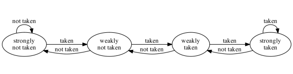
Figure 1: A 2-bit branch predictor behaves as shown in this finite-state automaton. Each node is a state representing the next prediction, e.g., the strongly and weakly taken states predict “taken,” the others, “not taken.” Each edge shows how the state changes once the actual branch condition is resolved.

Given a particular (static) conditional branch in a graph algorithm, our analysis goal is to estimate how many times the branch predictor will mispredict it.Although we do not know exactly what type of branch predictor a vendor implements, our analysis assumes a 2-bit branch predictor [46]. The empirical evaluation of § 6 will justify this choice. Like most branch prediction techniques, it uses the history of previous executions of a given branch to predict the next outcome; as such, one may formalize the analysis of predictors mathematically using Markov chains and reason about expected branch misses, which we have done. However, for concerns of readability and space, this paper omits the details of such analysis, instead stating the key results and offering more intuitive high-level explanations.

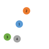
(a)

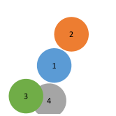
(b)

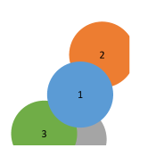
(c)

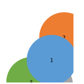
(d)

(e)

Figure 2: These sub-figures conceptually show how the connected component id propagates through the graph as time evolves - each subfigure is for a different iteration of the algorithm. This example assumes that all vertices are connected and for simplicity shows only the connected components are 1 through 4. Initially the number of connected components is equal to the number vertices. (a) Depicts the initial state in which each vertex is in its own component. (b)-(d) depict that some vertices belong to the same connected component yet may require multiple label updates (in either the same iteration or a separate iteration). (e) is the final state in which there is a single connected component.

Let $n\geq 0$;

$i\leftarrow 0$;

while $i<n$ do

       // … $i$, $n$ unmodified; no early exits …
$i\leftarrow i+1$;

      

Algorithm 1 A simple sequential while-loop, which executes its body exactly $n$ times

3.1 A model of 2-bit predictors

For each (static) conditional branch in the program, a 2-bit predictor maintains a 2-bit state value, which encodes four possible states. Each state value is a prediction for the next occurrence of this branch; once the true branch condition is known, this state is updated. The precise states and transitions appear in the finite-state automaton (FSA) of fig. 1. In particular, there are four possible states, named Strongly-Taken, Weakly-Taken, Weakly-Not-Taken, and Strongly-Not-Taken. The “strong” states reflect that the last few branches were all the same, i.e., all “taken” or all “not taken,” and so it is likely the next branch will be the same. The weak states allow for the predictor’s bias to change if a new pattern emerges.

We will further assume that the processor has enough branch state storage to track, for each conditional branch of interest, its 2-bit state for the duration of the program. That is, we will not consider the case when the processor runs out of branch state storage and must “evict” (and therefore losing or resetting) the branch state.

3.2 Analysis of simple loops

Several common programming patterns in graph algorithms are simple sequential loops, which iterate over, the set of vertices, edges, neighbors of a vertex, i.e., the adjacency list. Consider, for example, the simple sequential while-loop of alg. 1. By “simple,” we mean that (a) the iteration variable $i$ increases monotonically by 1 at each iteration; (b) the loop bound $n$ is constant as the loop executes; and (c) there are no early exits. Thus, this loop executes its body exactly $n$ times. The conditional branch in this case evaluates the condition, $i<n$. We will assume the convention for this loop is such that the branch is taken when the condition is true, and not taken when the condition is false. There will be exactly $n+1$ evaluations of this branch, only the last of which is not taken in order to exit the loop. We can state a number of facts about such loops, assuming the 2-bit branch predictor.

Lemma 1

When $n\geq 3$, the final state of the 2-bit predictor is Weakly-Taken.

Proof 3.1.

The conditional branch is taken $n$ times. In the worst case, we begin the loop in the Strongly-Not-Taken state. According to the FSA of fig. 1, after three taken state transitions, the predictor will be in the Strongly-Taken state. Since the final branch is not taken, the predictor must move into the Weakly-Taken state.

Lemma 3.2.

When $n\geq 3$, the maximum number of branch mispredictions incurred by the loop’s conditional test (ignoring conditional branches in the body) is 3.

Proof 3.3.

As with lemma 1, the the initial state of the predictor may be Strongly-Not-Taken, which will cause 2 mispredictions before reaching either of the Taken states. For the last loop iteration, when $i=n\geq 3$, the predictor will be in the Strongly-Taken state but branch will be taken, incurring one more branch miss. Thus, there could be up to 3 misses. Furthermore, there must be at least 1 branch miss, which occurs on the last (not taken) branch; the reason is that the predictor must be in the Strongly-Taken state by iteration $i=n-1$, independent of the initial state.

Lemma 3.4.

Suppose we execute the same loop $k\geq 2$ times (such as in the case of nested loops), where $n\geq 3$ on the first execution, and $n\geq 1$ on every subsequent execution. These are nested loops - $k$ designates the outer-loop and $n$ for the inner-loop. Then there may be up to $k+2$ mispredictions for the inner loop, that is, up to 3 misses during the first execution and 1 additional miss on each of the $k-1$ remaining executions.

Proof 3.5.

Based on lemma 1 the branch predictor is in the Weakly-Taken state at the end of the first execution of the loop and may see up to 3 mispredictions. This state becomes the initial state for the next execution. If $n\geq 1$ on every execution after the first, then the predictor will move to the Strongly-Taken state; on the last iteration, it will return to the Weakly-Taken state, incurring 1 misprediction. That is, we will bounce back-and-forth between Strongly-Taken and Weakly-Taken.

Corollary 3.6.

If $k\gg 2$, we should expect approximately $k$ branch misses.

Lemma 3.7.

Suppose $n=0$. Then the predictor will move toward the Strongly-Not-Taken state and cannot be in the Strongly-Taken state; furthermore, it will incur either 0 or 1 branch misses.

Lemma 3.8.

Suppose $n=1$. Then the predictor will return to its initial state, incurring either 1 or 2 branch misses.

Lemma 3.9.

Suppose $n=2$. Then the branch predictor must end in either the Weakly-Taken or Weakly-Not-Taken states, and will incur between 1 and 3 branch misses.

4 Connected Components

For the problem of finding connected components, we assume the Shiloach and Vishkin (SV) algorithm [44]. It has been implemented on numerous multiprocessor systems, including the massively threaded Cray XMT [1, 21] and a variety of x86 systems [36].

SV is based on a propagation technique, and its pseudocode appears in alg. 2. It maintains for each vertex $v$ a component label, $CC_{\_}{id}[v]$, and updates this label to place adjacent vertices into the same connected component. Initially, each vertex $v$ is placed into a connected component by itself, which by convention is a label equal to the vertex number. As such, there are a total of $|V|$ connected components at this stage. In the first iteration, each vertex $v$ compares its own label with each of its neighbors, $u\in\operatorname{adj}(v)$. Again by convention, the vertex replaces its own label with the minimum label among itself and its neighbors. The algorithm is iterative and stops when no further label changes occur, maintained by a flag.

Each iteration requires $O(|V|+|E|)$ computations, since the algorithm accesses all vertices and their respective adjacencies. The maximal length of propagation is limited by the graph diameter $d$. As such, the total time complexity of the algorithm is $O(d\cdot(|V|+|E|))$. Relative to alg. 2, there is a shortcut that can reduce the number of iterations to $d/2$ [44]. However, this does not change the asymptotic time complexity of the algorithm, and we do not consider it further.

Conceptually, the component labels propagate as fig. 2 depicts. Initially (a), four of the components have minimal labels locally; these labels propagate gradually, and the label of a given node may change several times, (b)-(e), possibly even within the same iteration. Eventually, the algorithm reaches a final state (e) where for a fully-connected graph there will be a single connected component.

// Algorithm initialization

for $v\in V$ do

       $CC_{\_}{id}[v]\leftarrow v$

$change\leftarrow 1$

// Connected component labeling

while $change\neq 0$ do

       $change\leftarrow 0$

      for $v\in V$ do

            

            $c_{\_}v\leftarrow CC_{\_}{id}[v]$

            for $u\in Neighbors[v]$ do

                  

                  $c_{\_}u\leftarrow CC_{\_}{id}[u]$

                  if $c_{\_}u\leq c_{\_}v$ then

                         $CC_{\_}{id}[v]\leftarrow c_{\_}u$

                        $change\leftarrow 1$

                  

            

      

Algorithm 2 Branch-based Shiloach-Vishkin algorithm for finding connect components.

// Algorithm initialization

for $v\in V$ do

       $CC_{\_}{id}[v]\leftarrow v$

$change\leftarrow 1$

// Connected component labeling

while $change\neq 0$ do

       $change\leftarrow 0$

      for $v\in V$ do

            

            $c_{\_}v^{init}\leftarrow CC_{\_}{id}[v]$

            $c_{\_}v\leftarrow c_{\_}v^{init}$

            for $u\in Neighbors[v]$ do

                  

                  $c_{\_}u\leftarrow CC_{\_}{id}[u]$

                  if $c_{\_}u\leq c_{\_}v$ then

                         $c_{\_}v\leftarrow c_{\_}u$

                  

            

            $CC_{\_}{id}[v]\leftarrow c_{\_}v$

            $change\leftarrow change\lor c_{\_}v\oplus c_{\_}v^{init}$

      

Algorithm 3 Branch-avoiding Shiloach-Vishkin algorithm for finding connect components.

4.1 Branch (Mis)predictions in SV

The standard version of the SV algorithm (alg. 2) has four static conditional branches. To analyze the branch mispredictions, we assume the 2-bit branch predictor model of § 3.

The first conditional branch is the termination test of the while statement. This condition is evaluated $d+1$ times, where $d$ is the diameter of the graph. Per § 3, assuming $d\geq 3$, it should incur at most 3 mispredictions, ignoring mispredictions in the body of the loop.

Next, consider the two conditional branches associated with the two for-loops. The first for-loop iterates over all vertices; the second for-loop iterates over all neighbors of each vertex, thereby effectively visiting all edges. From the facts of § 3.2, the first for-loop will incur up to 3 branch misses in total, assuming sufficiently large $|V|$. The second for-loop is an instance of a repeated loop (see lemma 3.4), which is executed $|V|$ times. Though the exact behavior of the inner loop depends on the degree distribution, we can estimate the misses by applying corr. 3.6, which implies approximately $|V|$ branch misses.

Finally, the if-statement is the hardest to analyze offline. The actual number of branch mispredictions will depend on the input graph. To get an idea, consider the example in fig. 2. In the first iterations, vertices are likely to “swap” their connected components multiple times, which complicates branch prediction as there may not be a regular pattern. As iterations proceed, labels begin to stabilize, making this condition more predictable. Thus, we should expect to see many mispredictions initially, gradually decreasing as iterations proceed.

4.2 Branch-avoiding SV

Algorithm 3 presents the pseudocode for a branch-avoiding algorithm for the Shiloach-Vishkin connected component formulation. This algorithm compares the values of the connected component ids; however does not branch based on the value of the comparison. Instead this approach uses a conditional move that copies the value into the variable $c_{\_}v$ if and only if the id of $u$ is smaller than the the value in $c_{\_}v$. For the Shiloach-Vishkin algorithm the value of the connected component of $v$ is stored in $c_{\_}v$ which is a register, meaning that the number of writebacks (stores) is $|V|$. To ensure the correctness of the algorithm and that the algorithm will stop at some point, the variable $change$ is updated using a bitwise OR of bitwise XOR between the initial $c_{\_}v^{init}$ and the updated $c_{\_}v$. If the value of the connected component changed for the current vertex, $c_{\_}v$ is not equal to $c_{\_}v^{init}$ and their XOR value is non-zero. Accordingly, if any connected component changed, $change$ variable will have non-zero after traversing vertices in $V$.

5 Breadth First Search

$Q\leftarrow$ empty queue;

initialize $d[v\in V]\leftarrow\infty$;

enqueue $r\rightarrow Q$;

set $d[r]\leftarrow 0$;

while $Q$ not empty do

       dequeue $v\leftarrow Q$;

       for all neighbor $w$ of $v$ do

            

            if $d[w]=\infty$ then // $w$ found for the first time

                   $enqueue\,w\rightarrow Q$;

                   $d[w]\leftarrow d[v]+1$;

                  

            

      

Algorithm 4 Pseudocode for branch-based Breadth First Search starting from a vertex $r$

$Q\leftarrow$ empty queue;

$Q_{\_}{len}\leftarrow 1$; initialize $d[v\in V]\leftarrow\infty$;

enqueue $r\rightarrow Q$;

set $d[r]\leftarrow 0$;

while $Q$ not empty do

       dequeue $v\leftarrow Q$;

       $next\_level\leftarrow d[v]+1$; for all neighbor $w$ of $v$ do

            

            $LOAD(temp,d[w])$;

             $CMP(temp,d[v])$;

             $Q[Q_{\_}{len}]\leftarrow w$;

             $COND\_MOVE\_GREATER(temp,next\_level)$;

             $COND\_ADD(Q_{\_}{len},1)$;

             $STORE(temp,d[w])$;

            

      

Algorithm 5 Pseudo code for branch-avoiding Breadth First Search

Given a graph and a root vertex $r$, a breadth-first search (BFS) computes the distance of every node in the graph to $r$. The pseudocode for the BFS algorithm we consider appears in alg. 4.

5.1 Branch (Mis)predictions in BFS

The BFS algorithm of alg. 4 has three branches: (while), (for), and (if). We consider the impact of branch mispredictions assuming a 2-bit branch predictor. In particular, we estimate a practical lower bound on the number of branch misses. We validate this estimate in § 6.

The first branch, (while), is used to iterate through the queue of vertices in the current and next frontiers. For a breadth first search that finds the vertices $\hat{V}$, s.t. $\hat{V}\subseteq V$ , the condition of the while branch will be evaluated a total of $|\hat{V}|+1$ times. Based on the lemmas of § 3.2 the number of branch misprediction for this statement is $O(1)$.

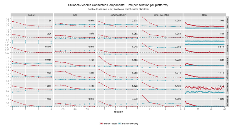
Figure 3: Time as a function of the iteration for the Shiloach-Vishkin algorithm.

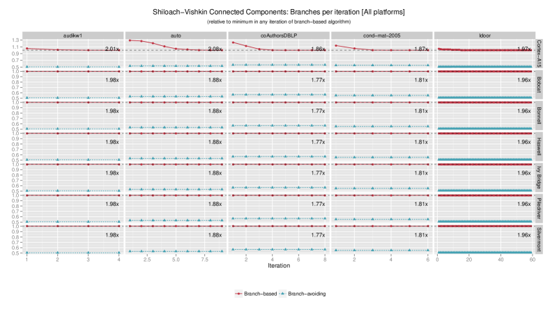
Figure 4: Branches as a function of the iteration for the Shiloach-Vishkin algorithm.

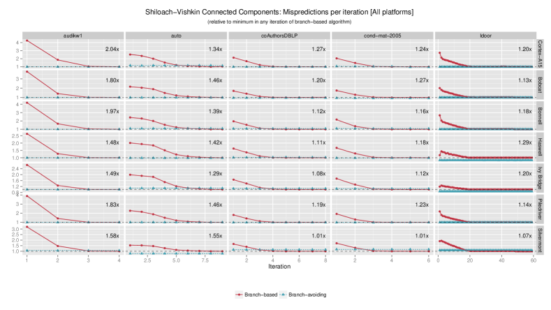
Figure 5: Branch mispredictions as a function of the iteration for the Shiloach-Vishkin algorithm.

The second conditional branch, the for statement, is responsible for traversing the adjacency list of a given vertex. Based on the lemmas from § 3.2, as this loop is executed $\hat{V}$ times, there should be approximately $\hat{V}$ misses. For undirected graphs, each vertex found in the BFS traversal has at least on vertex that will be traversed. For directed graphs a situation can arise that a vertex does not have any outbound adjacencies. In practice, there should be nearly $|\hat{V}|$ branch misses for the for statement.

The last of these conditions, the if statement, checks if a vertex has been found. As each vertex can be found only once, this branch will be taken at most $|\hat{V}|$ times. This branch statement is evaluated $|\hat{E}|$ times where $\hat{E}\subseteq E\wedge\hat{E}={((v,u)|v\in\hat{V}})$. The exact order in which this branch will be $TAKEN$ is highly dependent on the order in which the vertices and edges are accessed. For example, when the neighbors of the root are traversed, they will all be added to the queue (i.e. branch TAKEN) and there will be fewer misses. Now consider the neighbors of the root, these might have some common neighbors in the second frontier, however, only the first traversal of the common neighbor will take the branch. In the worst case a scenario can arise in which the state of the if branch moves back and forth between WEAKLY-NOT-TAKEN and WEAKLY-TAKEN. This can potentially double the number of branch misses for the if branch. As such the if statement can have upto $2\cdot|\hat{V}|$ branch misses.

Thus the upper-bound on the number of branch misses for the branch-based algorithm is $3\cdot|\hat{V}|+O(1)$.

5.2 Branch Avoiding BFS

Algorithm 5 presents the pseudocode for a BFS branch-avoiding algorithm. Similar to the Shiloach-Viskin algorithm a compare without branch is used to compare the level of the current vertex with the level of its adjacency. The adjacent vertex, $w$, is placed at the end of the queue. Based on hardware flags, two conditional operations are completed. The first will conditionally move the distance to the vertex if it is found for the first time. The second conditional operation increases the size of the queue. If an element is new then the queue size is increased and the element is enqueued. If the vertex is not new, then it has been placed “outside” the queue and will be overwritten when a new vertex is found. When this is done the distance of $w$ is written back to. This means that there are $O(E)$ writebacks.

6 Empirical Results

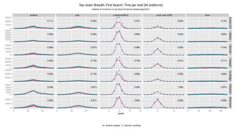
Figure 6: Time as a function of the iteration for BFS.

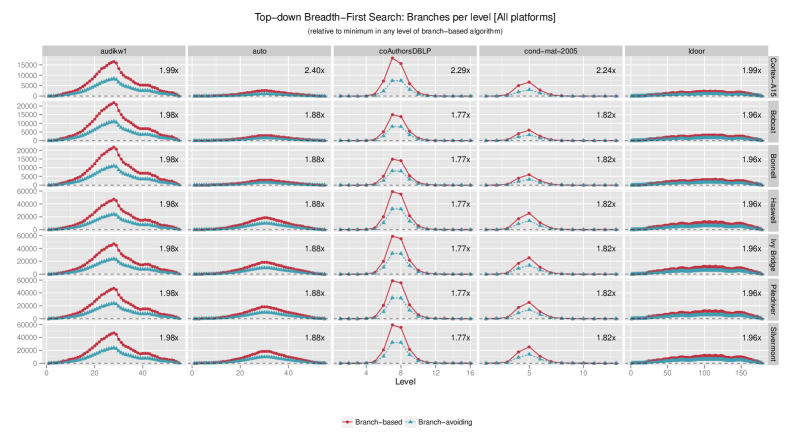
Figure 7: Branches as a function of the iteration for BFS.

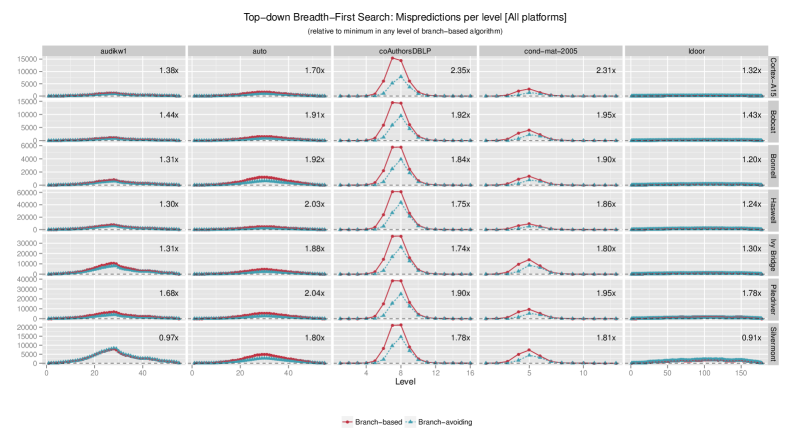
Figure 8: Branch mispredictions as a function of the iteration for BFS.

Table 1: Systems used in experiments.

Architecture	Microarchitecture	Processor	Frequency	L1 Cache	L2 Cache	L3 Cache	DRAM Type
ARM v7-A	Cortex-A15 [arn]	Samsung Exynos 5250	1.7 GHz	32 KB	1 MB		SC DDR3-800
x86-64	Piledriver [pld]	AMD FX-6300	3.5 GHz	16 KB	2 MB	8 MB	DC DDR3-1600
x86-64	Bobcat	AMD E2-1800	1.7 GHz	32 KB	512 KB		SC DDR3-1333
x86-64	Haswell [hsw]	Intel Core i7-4770K	3.5 GHz	32 KB	256 KB	8 MB	DC DDR3-2133
x86-64	Ivy-Bridge [ivb]	Intel Core i3-3217U	1.8 GHz	32 KB	256 KB	3 MB	DC DDR3-1600
x86-64	Silvermont [slv]	Intel Atom C2750	2.4 GHz	24 KB	1 MB		DC DDR3-1600
x86-64	Bonnell	Intel Atom 330	1.6 GHz	24 KB	512 KB		SC DDR3-800

Table 2: Graphs from the 10th DIMACS Implementation Challenge used in our experiments.

Name	Graph Type	$|V|$	$|E|$
audikw1	Matrix	943,695	38,354,076
auto	Partitioning	448,695,	3,314,611
coAuthorsDBLP	Collaboration	299,067	977,676
cond-mat-2005	Clustering	40,421	175,691
ldoor	Matrix	952,203	22,785,136

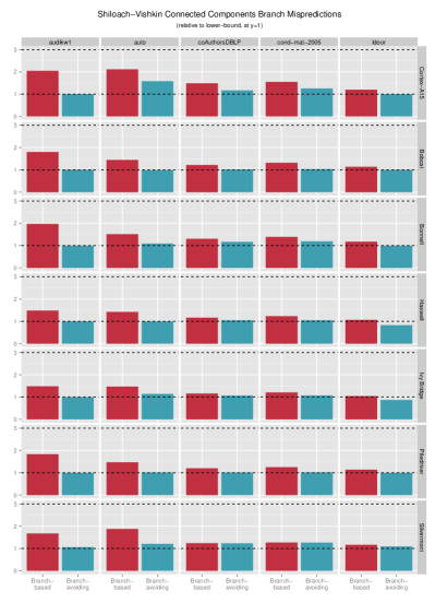
(a)

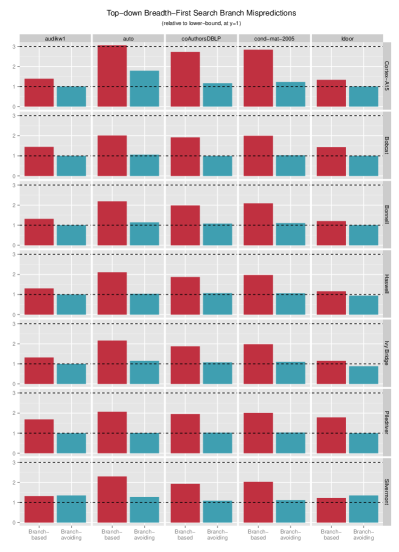
(b)

Figure 9: Lowerbounds on the number of branch mispredictions for SV (based on the model given in Section 4) and BFS (based on the model given in Section 5) . The bars for each algorithm show the ratio of branch mispredictions in comparison to the lower bound. For BFS, an upper bound is also provided.

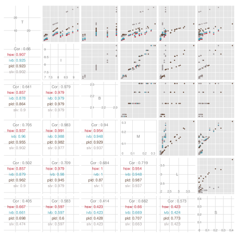
(a)

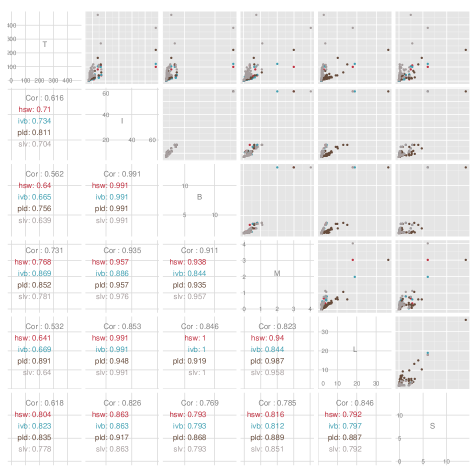
(b)

Figure 10: Correlations among time (T), instructions (I), branches (B), mispredictions (M), load operations (L), and store operations (S) per edge, both for (a) SV, and (b) BFS. Each sample is a different iteration/level for one of the graph.

6.1 Experimental Setup

For experimental evaluation we tried several implementations of Shiloach-Vishkin connected components algorithm and the top-down breadth-first search algorithm for x86-64 and ARM architectures. Unfortunately, compilers do not provide explicit control over the use of branches or conditional moves in the generated code, which complicated our analysis. The x86-64 systems compilers tended to generate conditional branches when conditional moves could be used; albeit we found two ways to make compilers avoid branches, both of them involved inefficiencies: 1) inline assembly allowed manual selection of instructions; however the compilers generated suboptimal code around the inlined assembly; 2) force the compiler to use SETcc instructions by storing the result of the comparison into a byte variable followed by extending the bit mask for conditional selection - this approach caused the compiler to generate $8-9$ instructions where a single CMOVcc instruction could suffice. On the ARM system we had a reverse problem: instead of a conditional branch or move, compilers preferred to use conditional store instructions, which impose big performance penalty on Cortex-A15.

For better control of generated code we implemented both connected components and breadth-first search algorithms in x86-64 and ARM assembly using the PeachPy [19] framework. We performed our experiments on $7$ systems with different microarchitectures, these are presented in Table 1. On all systems the assembly implementations performed at least as well as C implementations. The algorithms were tested on graphs taken from the DIMACS 10 Graph Challenge [2], detailed in Table 2.

6.2 Connected Components

Fig. 3 depicts the ratio of the execution times as a function of the iteration for the Shiloach-Vishkin algorithm on the systems in tab. 1. The ratio for each of the algorithm is between the execution time of a given iteration and the fastest iteration of the branch-based algorithm. The branch-based algorithm is depicted by the red curve and the branch-avoiding algorithm is depicted by the blue curve. The abscissa for these figures is the iteration of the algorithm. In each subfigure the total speedup of the branch-avoiding algorithm over the branch-based algorithm is given. Note that for several of the iterations the difference between the branch-based algorithm and the branch-avoiding is high as $30\%-50\%$, with the branch-avoiding algorithm being the faster of these. In a handful of cases, specifically on the Bonnell system, the branch-based algorithm is $20\%$ faster than the branch-avoiding algorithm.

Recall that as the connected component id propagates in the graph fewer vertices change their connected component - this also makes the branch predictor job easier as it will accurately predict the condition. Fig. 4 and Fig. 5 depict the ratio of branches and number of branch mispredictions as a function of the iteration, respectively.

On some systems, for example Cortex-A15 , the branch-avoiding algorithm offers better performance for all iterations of the algorithm over all the graphs. While for some systems, in the initial iterations the branch-avoiding algorithms offers better performance and in the later iterations the branch-based algorithm gives better performance. This is both system- and graph-dependent. In the case that there is a crossover point for performance dominance of the algorithms, it is a single crossover point from where the branch-avoiding algorithm is initially faster to where the branch-based is faster in the later iterations. The significance of the single crossover point is that this may allow creating a hybrid algorithm that uses the faster of the two algorithms based on the iteration.

Fig. 4 shows that the branch-based algorithm has nearly double the number of branches than the branch-avoiding algorithm. For the Intel and AMD systems, the number of branches is constant throughout the iterations while for the Cortex-A15 system it is not. For the Intel and AMD systems, the hardware counter returns the number of retired branch instructions while the ARM system returns the number of dispatched branches. Due to the higher misprediction rate in the first iterations, the number of dispatched branches is also higher as these are flushed instructions.

The branch-based algorithm can potentially have as many as 4X the number of branch mispredictions as that of the branch-avoiding algorithm, fig. 5. In all cases the branch-avoiding algorithm has fewer branches and branch mispredictions. Note, for most graphs, the ratio between the total number of mispredictions for the two algorithms (denoted by the number at the top-right corner of each subfigure) for a given graph is within a small region for all systems.

Fig. 9 (a) depicts the ratio of the total number of branch mispredictions for the two algorithm versus the lower-bound on the number of branch mispredictions. The lower-bound is denoted with a black line at y=1 and this is equal to the lower-bound presented in § 4 for the 2-bit branch-predictor. For most systems, the branch-avoiding algorithms is near the lower-bound, while the branch-based algorithm is well above this line. For the Cortex-A15 system, there are three different graphs in which the branch misprediction rate is well above the lower-bound, for the $auto$ graph the branch misprediction rate is $50\%$ above the lower-bound. This means that implemented branch-predictor in fact increases the misprediction rate. Both the Bonnell and the Silvermont systems also have higher than lower-bound miss rate for several of the graphs. However, these are lower than the miss rate of the Cortex-A15 system.

6.3 Breadth First Search

Fig. 6 depicts the ratio of the execution times as a function of the iteration for BFS. The ratio for each of the algorithm is between the execution time of a given iteration and the fastest iteration of the branch-based algorithm. The branch-based algorithm is depicted by the red curve and the branch-avoiding algorithm is depicted by the blue curve. The abscissa for these figures is the iteration of the algorithm. In each subfigure the total speedup of the branch-avoiding algorithm over the branch-based algorithm is given. In most cases the branch-avoiding algorithm does not offer a speedup and in fact causes a slowdown for BFS. The branch-avoiding algorithm performs the best on the Silvermont system where it is faster for 4 out the 5 test cases.

Fig. 7 depicts the ratio of the number of branches of the branch-based algorithm with the branch-avoiding algorithm. Fig. 8 depicts the ratio of the number of branches mispredictions of the branch-based algorithm with the branch-avoiding algorithm. Note the similarity of these figures with the time per iteration, fig. 6. Also, note that the branch-based algorithm has nearly double the number of branches than the branch-avoiding algorithm. If one considers the average number of branches per edge traversal in each frontier, these ratios are still maintained.

Fig. 9 (b) depicts the ratio of the total number of branch mispredictions for the two algorithm versus the lower-bound on the number of branch mispredictions. The lower-bound is denoted with a black line at y=1 and the upper-bound is denoted with a black line at y=3. The upper and lower bounds on the number of branch mispredcition for a 2-bit branch predictor BFS was discussed in § 4. The lower-bound is dependent on the number of vertices found in the traversal, $\hat{V}$ and the upper bound is 3 times the lower-bound. Similar to the Shiloach-Vishkin algorithm, the branch-avoiding algorithms is near the lower-bound for most graphs and on most systems. Again, the Cortex-A15 system has some of the higher misprediction rates for both algorithms.

6.4 The effects of misprediction

To get an idea of how strongly mispredictions influence performance, we show pairwise correlations among the a priori most likely predictors of execution time: instructions, loads, stores, and based on the subject of this paper, branches and branch mispredictions. Fig. 10 shows this data for the branch-based versions of both SV (left half) and BFS (right half). Each $6\times 6$ grid of subplots shows the correlations among time, instructions, branches, mispredictions, loads, and stores, measured per edge traversal. For example, (row 1, column 2) subplot in each half is a scatter plot comparing time (“T”) on the y-axis with instructions (“I”) on the x-axis. The points are color-coded by platform, on the subset of platforms that supported all necessary hardware performance counters. For each $(R,C)$ plot in the upper-triangle, the computed correlation coefficients appear in the transposed $(C,R)$ position of the lower-triangle.

In the case of SV, mispredictions more strongly correlate with time than instructions, branches, loads, and stores. Though not a strict proof-of-cause, this observation is nevertheless somewhat surprising, as it implies mispredictions may be nearly or even more important than memory behavior. By contrast, in the case of BFS, the correlations with stores and mispredictions is roughly equal, with stores being slightly more strongly correlated than time. This confirms the performance behavior seen previously, namely, that eliminating branches at the cost of increasing stores should not be expected to improve performance. In practice the number of stores were increased by two order of magnitude for some graphs.

7 Conclusions

On the one hand, our study is a positive result for the branch-avoiding technique in the case of SV, where mispredictions are more strongly correlated to time than even memory traffic, much to our surprise. This raises the question of whether branch-avoidance might be important in other computations, and whether increased microarchitectural support for predication-like instructions might have more significant benefits.

On the other hand, our study is a negative result for BFS. Stores are as critical as branch mispredictions, so the tradeoff that reduces branches at the cost of significantly increasing stores cannot pay off. One question is why: although total stores increased by much as $100\times$, the actual slowdown was always $2\times$ or less. Indeed, the extra stores are purely “local” in that they should mostly hit in cache, by design of the implementation. Thus, there is a potential in the microarchitecture to address whatever resource constraints the additional stores impose, such as buffers for more outstanding operations.

An additional question is to what extent compiler transformations can or should replicate the transformations we implemented by hand. Though not shown explicitly, although the ARM system supported predicated instructions, no compiler produced transformations equivalent to our hand-generated code. Whether the gap can be filled remains open, in our view.

References

- [1] GraphCT: A Graph Characterization Toolkit.
- [2] 10th dimacs implementation challenge - graph partitioning and graph clustering, 2013.
- [3] R. Albert, H. Jeong, and A. Barab si. Internet: Diameter of the world-wide web. Nature, 401(6749):130–131, Sep 09 1999.
- [4] D. A. Bader, J. Berry, A. Amos-Binks, D. Chavarría-Miranda, C. Hastings, K. Madduri, and S. C. Poulos. STINGER: Spatio-Temporal Interaction Networks and Graphs (STING) Extensible Representation. Technical report, Georgia Institute of Technology, 2009.
- [5] D. A. Bader and K. Madduri. Designing multithreaded algorithms for breadth-first search and st-connectivity on the Cray MTA-2. In Parallel Processing, 2006. ICPP 2006. International Conference on, pages 523–530. IEEE, 2006.
- [6] A.-L. Barab si and R. Albert. Emergence of scaling in random networks. Science, 286(5439):509–512, 1999.
- [7] B. W. Barrett, J. W. Berry, R. C. Murphy, and K. B. Wheeler. Implementing a portable multi-threaded graph library: The MTGL on Qthreads. In Parallel & Distributed Processing, 2009. IPDPS 2009. IEEE International Symposium on, pages 1–8. IEEE, 2009.
- [8] S. Beamer, K. Asanovic, and D. Patterson. Direction-optimizing breadth-first search. In High Performance Computing, Networking, Storage and Analysis (SC), 2012 International Conference for, pages 1–10. IEEE, 2012.
- [9] S. Beamer, A. Buluç, K. Asanovic, and D. Patterson. Distributed memory breadth-first search revisited: Enabling bottom-up search. In Proceedings of the 2013 IEEE 27th International Symposium on Parallel and Distributed Processing Workshops and PhD Forum, pages 1618–1627. IEEE Computer Society, 2013.
- [10] U. Brandes. A faster algorithm for betweenness centrality. Journal of Mathematical Sociology, 25(2):163–177, 2001.
- [11] A. Broder, R. Kumar, F. Maghoul, P. Raghavan, S. Rajagopalan, R. Stata, A. Tomkins, and J. Wiener. Graph structure in the Web. Computer Networks, 33:309 – 320, 2000.
- [12] A. Buluç and K. Madduri. Parallel breadth-first search on distributed memory systems. In Proceedings of 2011 International Conference for High Performance Computing, Networking, Storage and Analysis, page 65. ACM, 2011.
- [13] A. Bulu and J. R. Gilbert. The Combinatorial BLAS: design, implementation, and applications. International Journal of High Performance Computing Applications, 25(4):496–509, 2011.
- [14] M. Burtscher, R. Nasre, and K. Pingali. A quantitative study of irregular programs on GPUs. In Workload Characterization (IISWC), 2012 IEEE International Symposium on, pages 141–151. IEEE, 2012.
- [15] F. Checconi, F. Petrini, J. Willcock, A. Lumsdaine, A. R. Choudhury, and Y. Sabharwal. Breaking the speed and scalability barriers for graph exploration on distributed-memory machines. In High Performance Computing, Networking, Storage and Analysis (SC), 2012 International Conference for, pages 1–12. IEEE, 2012.
- [16] J. Chhugani, N. Satish, C. Kim, J. Sewall, and P. Dubey. Fast and efficient graph traversal algorithm for CPUs: Maximizing single-node efficiency. In Parallel & Distributed Processing Symposium (IPDPS), 2012 IEEE 26th International, pages 378–389. IEEE, 2012.
- [17] G. Cong and K. Makarychev. Optimizing large-scale graph analysis on multithreaded, multicore platforms. In Parallel & Distributed Processing Symposium (IPDPS), 2012 IEEE 26th International, pages 414–425. IEEE, 2012.
- [18] T. H. Cormen, C. E. Leiserson, R. L. Rivest, and C. Stein. Introduction to Algorithms. The MIT Press, New York, 2001.
- [19] M. Dukhan. PeachPy: A python framework for developing high-performance assembly kernels.
- [20] A. N. Eden and T. Mudge. The YAGS branch prediction scheme. In Proceedings of the 31st annual ACM/IEEE international symposium on Microarchitecture, pages 69–77. IEEE Computer Society Press, 1998.
- [21] D. Ediger, K. Jiang, J. Riedy, and D. Bader. Graphct: Multithreaded algorithms for massive graph analysis. Parallel and Distributed Systems, IEEE Transactions on, PP(99):1–1, 2012.
- [22] D. Ediger, R. McColl, J. Riedy, and D. Bader. Stinger: High performance data structure for streaming graphs. In Proc. High Performace Embedded Computing Workshop (HPEC 2012), Waltham, MA, Sept. 2012.
- [23] M. Faloutsos, P. Faloutsos, and C. Faloutsos. On Power-Law Relationships of The Internet Topology. In ACM SIGCOMM Computer Communication Review, pages 251–262. ACM, 1999.
- [24] R. W. Floyd. Algorithm 97: Shortest path. Commun. ACM, 5:345–345, June 1962.
- [25] A. Fog. The microarchitecture of Intel, AMD and VIA CPUs. An optimization guide for assembly programmers and compiler makers. Copenhagen University College of Engineering, 2013.
- [26] L. C. Freeman. A set of measures of centrality based on betweenness. Sociometry, 40(1):pp. 35–41, 1977.
- [27] O. Green, R. McColl, and D. A. Bader. A Fast Algorithm For Streaming Betweenness Centrality. In Proceedings of the 4th ASE/IEEE International Conference on Social Computing, SocialCom ’12, 2012.
- [28] D. Gregor and A. Lumsdaine. The parallel BGL: A generic library for distributed graph computations. Parallel Object-Oriented Scientific Computing (POOSC), page 2, 2005.
- [29] S. Hong, H. Chafi, E. Sedlar, and K. Olukotun. Green-Marl: a DSL for easy and efficient graph analysis. In ACM SIGARCH Computer Architecture News, volume 40, pages 349–362. ACM, 2012.
- [30] J. Hopcroft and R. Tarjan. Algorithm 447: efficient algorithms for graph manipulation. Commun. ACM, 16(6):372–378, June 1973.
- [31] G. Karypis and V. Kumar. Metis-unstructured graph partitioning and sparse matrix ordering system, version 2.0. 1995.
- [32] C.-C. Lee, I.-C. Chen, and T. N. Mudge. The bi-mode branch predictor. In Microarchitecture, 1997. Proceedings., Thirtieth Annual IEEE/ACM International Symposium on, pages 4–13. IEEE, 1997.
- [33] J. K. Lee and A. J. Smith. Branch prediction strategies and branch target buffer design. Computer, 17(1):6–22, 1984.
- [34] J. Leskovec, J. Kleinberg, and C. Faloutsos. Graph evolution: Densification and shrinking diameters. ACM Trans. Knowl. Discov. Data, 1(1), 2007.
- [35] G. Malewicz, M. H. Austern, A. J. Bik, J. C. Dehnert, I. Horn, N. Leiser, and G. Czajkowski. Pregel: a system for large-scale graph processing. In Proceedings of the 2010 ACM SIGMOD International Conference on Management of data, pages 135–146. ACM, 2010.
- [36] R. McColl, O. Green, and D. Bader. Parallel streaming connected components using “parent-neighbor” subgraphs. In IEEE International Conference on High Performance Computing, 2013.
- [37] D. Merrill, M. Garland, and A. Grimshaw. Scalable gpu graph traversal. In ACM SIGPLAN symposium on Principles and Practice of Parallel Programming, PPoPP ’12, pages 117–128, New York, NY, USA, 2012. ACM.
- [38] M. Milenkovic, A. Milenkovic, and J. Kulick. Demystifying intel branch predictors. In Workshop on Duplicating, Deconstructing and Debunking, 2002.
- [39] S. Milgram. The Small World Problem. Psychology Today, 2(1):60–67, 1967.
- [40] M. Newman and M. Girvan. Finding and evaluating community structure in networks. Physical review E, 69(2):026113, 2004.
- [41] E. J. Riedy, H. Meyerhenke, D. Ediger, and D. A. Bader. Parallel community detection for massive graphs. In Parallel Processing and Applied Mathematics, pages 286–296. Springer, 2012.
- [42] G. Sabidussi. The centrality index of a graph. Psychometrika, 31(4):581–603, 1966.
- [43] Y. Shiloach and S. Even. An on-line edge-deletion problem. J. ACM, 28:1–4, January 1981.
- [44] Y. Shiloach and U. Vishkin. An O(logn) parallel connectivity algorithm. Journal of Algorithms, 3(1):57 – 67, 1982.
- [45] J. Shun and G. E. Blelloch. Ligra: a lightweight graph processing framework for shared memory. In Proceedings of the 18th ACM SIGPLAN symposium on Principles and practice of parallel programming, pages 135–146. ACM, 2013.
- [46] J. E. Smith. A study of branch prediction strategies. In Proceedings of the 8th annual symposium on Computer Architecture, pages 135–148. IEEE Computer Society Press, 1981.
- [47] E. Sprangle, R. S. Chappell, M. Alsup, and Y. N. Patt. The agree predictor: A mechanism for reducing negative branch history interference. In ACM SIGARCH Computer Architecture News, volume 25, pages 284–291. ACM, 1997.
- [48] S. Warshall. A theorem on boolean matrices. J. ACM, 9:11–12, Jan. 1962.
- [49] D. J. Watts and S. H. Strogatz. Collective Dynamics of “Small-World” Networks. Nature, 393(6684):440–442, 1998.
- [50] T.-Y. Yeh and Y. N. Patt. Two-level adaptive training branch prediction. In Proceedings of the 24th annual international symposium on Microarchitecture, pages 51–61. ACM, 1991.
- [51] T.-Y. Yeh and Y. N. Patt. Alternative implementations of two-level adaptive branch prediction. In ACM SIGARCH Computer Architecture News, volume 20, pages 124–134. ACM, 1992.
- [52] A. Yoo, E. Chow, K. Henderson, W. McLendon, B. Hendrickson, and U. Catalyurek. A scalable distributed parallel breadth-first search algorithm on BlueGene/L. In Supercomputing, 2005. Proceedings of the ACM/IEEE SC 2005 Conference, pages 25–25. IEEE, 2005.