Topology density correlator on dynamical domain-wall ensembles with nearly frozen topological charge

Abstract:

Global topological charge decorrelates very slowly or even freezes in fine lattice simulations. On the other hand, its local fluctuations are expected to survive and lead to the correct physical results as long as the volume is large enough. We investigate this issue on recently generated configurations including dynamical domain-wall fermions at lattice spacings $a=0.08$ fm and finer. We utilize the Yang-Mills gradient flow to define the topological charge density operator and calculate its long-distance correlation, through which we propose a new method for extracting the topological susceptibility in a sub-volume. This method takes care of the finite volume correction, which reduces the bias caused by the global topological charge. Our lattice data clearly show a shorter auto-correlation time than that of the naive definition using the whole lattice, and are less sensitive to the global topological history. Numerical results show a clear sea-quark mass dependence, which agrees well with the prediction of chiral perturbation theory.

1 Introduction

The configuration space of continuum QCD is not smoothly connected, and divided into sectors characterized by the global topological charge $Q$. They are separated by infinitely high barriers of the gauge action. On the lattice, the barriers become finite, and the Monte Carlo simulation can sample the configurations at different topological charges. As approaching the continuum limit, however, the barriers grow rapidly so that the hybrid Monte Carlo updates cannot frequently go across these topological boundaries. As a consequence, the auto-correlation time of topological charge becomes very long already at a lattice spacing $a\sim 0.05$ fm [1, 2].

In our previous simulations [3, 4, 5] with the overlap quarks, we took this property as an advantage and performed the QCD simulations in fixed topological sectors. Avoiding the topological boundaries is effective to reduce the numerical cost for the overlap quark determinant which has discontinuities on the boundaries. This can be achieved by introducing an extra Wilson fermion determinant with a negative cut-off scale mass, which prevents the index of the overlap operator to change along the Monte Carlo history [6]. We developed a method to correct the fixed topology effects, and succeeded in extracting the topological susceptibility from the local topological fluctuation in the simulation with a fixed global topological charge [3, 4].

We have recently launched a new project of simulating QCD with chiral fermions on finer and larger lattices [7]. Our goal is to cover the lattice size of around 2.5–4 fm with the cut-off $1/a\sim$ 2.4–4.5 GeV. We employ the Möbius domain-wall fermions [8] which is numerically less expensive than the overlap fermions, while keeping the violation of the Ginsparg Wilson relation still small at the $0.1$% level compared to the cut-off. It turned out that this size of violation is sufficient to smooth out the quark determinant and the hybrid Monte Carlo has no obstacle in crossing the barriers. The problem of the long autocorrelation time exists as with other fermion formulations since the topology barriers due to the gauge action remains.

Since the effect of the global topological charge is nothing but a finite volume effect [9, 10], once it is removed, the auto-correlation associated with it could also be removed. Since the physical effect of the topological charge should be found in its local excitations [11, 12], in this work, we consider the local fluctuation of topology using the topological charge density operator constructed via the gauge links after performing the Wilson flow. As shown in Ref. [13], gluonic quantities after the gradient flow are free from UV divergences, and the gluonic definition of the topological charge density is closer to the continuum limit as the gauge fields become smoother after the flow.

With this gluonic construction, we propose a new method for extracting the topological susceptibility. Its definition is given in a sub-volume, and contains an $1/V$ correction term, to reduce the bias caused by the global topological charge. Our lattice data show a much shorter auto-correlation time than that of the naive calculation of the topological susceptibility summed over the whole lattice sites. We also find that our data indeed cancel the bias from the global topological charge. Moreover, the numerical results show a clear sea-quark mass dependence, which agrees well with the prediction of chiral perturbation theory.

2 A new method for extracting the topological susceptibility

In a finite volume $V$ the effect of the global topological charge $Q$ to any quantity is given by a series of $Q^{2}/V$, as well as $1/\chi_{t}V$ provided that the volume is sufficiently larger than the inverse of the topological susceptibility $\chi_{t}$. More explicitly, the expectation value of any CP-even operator $O$ in a fixed topological sector of $Q$ can be expressed by a series [9, 10]

$$\langle O\rangle_{Q}=\langle O\rangle_{\theta=0}+\left.\frac{\partial^{2}}{\partial\theta^{2}}\langle O\rangle_{\theta}\right|_{\theta=0}\times\frac{1}{2\chi_{t}V}\left[1-\frac{Q^{2}}{\chi_{t}V}\right]+\cdots,$$ (1)

when $\chi_{t}V\gg 1$. This is intuitively understood from the clustering property of quantum field theory that only nearby region can affect the local observables. Therefore, it is sufficient to measure any physical observable in a sub-volume, as long as the size of the sub-volume is larger than the correlation length of the system. Even the topological susceptibility is not an exception.

Suppose we have a good definition of the topological charge density operator $q(x)$. The topological susceptibility is conventionally defined by

$$\chi_{t}=\int d^{4}x\langle q(x)q(0)\rangle.$$ (2)

Using the clustering property and the fact that the lowest energy state couples to $q(x)$ is the eta-prime meson (with the mass $m_{\eta^{\prime}}$), one can truncate the integral at some radius $r_{\rm cut}(>1/m_{\eta^{\prime}})$:

$$\int_{|x|<r_{\rm cut}}d^{4}x\langle q(x)q(0)\rangle=\chi_{t}+\mathcal{O}(e^{-m_{\eta^{\prime}}r_{\rm cut}}).$$ (3)

When the configurations are generated in a fixed topological sector or in various sectors but their distribution is rather biased, there are potential effects from the badly sampled $Q$ as $1/V$ corrections. Thus, it is better if one can subtract this correction in advance. Luckily, in the case of topological susceptibility, one can uniquely determine this correction term with no free parameter to tune. Namely, at long distances $|x|>r_{\rm cut}$, the correlator $q(x)q(0)$ in the topological sector of $Q$ is determined purely by the finite volume effects due to $Q$ [10],

$$\langle q(x)q(0)\rangle_{Q}\sim\frac{1}{V}\left[\frac{Q^{2}}{V}-\chi_{t}\right].$$ (4)

Even when the sampling of the configuration has a bias in the global topological charge $Q$, its effect can be subtracted, according to this formula. This is achieved by calculating

$$\bar{\chi}_{t}=\frac{V}{V-V_{\rm sub}}\left\langle\int_{|x|<r_{\rm cut}}d^{4}x\;q(x)q(0)-\frac{V_{\rm sub}}{V^{2}}Q^{2}\right\rangle,$$ (5)

where $V_{\rm sub}$ is the volume of the sub-domain in the range $|x|<r_{\rm cut}$. Note that $\chi_{t}=\bar{\chi_{t}}$ when the sampling of the topology has no bias. Since $\bar{\chi}_{t}$ is defined in a sub-volume, we can use the translational invariance and average it over the whole volume, which reduces the statistical uncertainty, and assures that the smooth limit $\displaystyle\lim_{V_{\rm sub}\to V}\bar{\chi_{t}}=\chi_{t}$ even for finite statistics of the gauge samples.

We expect that $\bar{\chi}_{t}$ has a shorter auto-correlation time than $\chi_{t}$ for two reasons. First, the topological lump can freely go in and out of the sub-domain whose moving time-scale is reported to be much shorter than $Q$ [14]. Second, the bias from global topology history is removed in advance, and the measurement should be insensitive to the (biased) history of the global topology.

The above observation is expected to be true only when we have a good definition of $q(x)$. For example, a naive pseudoscalar operator made from the plaquette on the generated configuration does not work very well. This is a part of the reason why conventionally the topological susceptibility has been measured by the global topological charge as $\langle Q^{2}\rangle/V$. In this work, we apply the Wilson flow cooling and use a naive gluonic definition of the topological charge density after the flow [13]. Any gluonic operator on the configurations cooled by the gradient flow has been shown to be free from UV divergences [13]. Moreover, if the plaquette values become sufficiently smooth, one can uniquely determine the global topological charge by a gluonic quantity. As we will see below, $q(x)$ after the gradient flow at the smearing range $\sim 0.5$ fm shows the expected properties.

3 Lattice simulation and Yang-Mills gradient flow

For the configuration generation, we employ the Symanzik gauge action and the Möbius domain-wall fermion action. The determinant of the Möbius domain-wall Dirac operator is equivalent to that of an approximation of the overlap Dirac operator:

$$D(m) = \frac{1+m}{2}+\frac{1-m}{2}\tanh(L_{s}\tanh^{-1}(2H_{T})),\;\;\;\;2H_{T}=\gamma_{5}\frac{2D_{W}}{2+D_{W}},$$ (6)

where $L_{s}$ is the size of 5-th direction, $D_{W}$ is the Wilson Dirac operator, and $m$ is the quark mass. We apply three steps of stout smearing of the gauge link before inserting it in the Dirac operator.

We carry out $2+1$-flavor lattice QCD simulations on two different lattice volumes $L^{3}\times T(\times L_{s})$=$32^{3}\times 64(\times 12)$ and $48^{3}\times 96(\times 8)$, for which we set $\beta=4.17$ and 4.35, respectively. The lattice spacings are estimated to be 2.4 GeV and 3.6 GeV, respectively, and therefore, the two lattices share a similar physical size. For the quark mass, we use two values of the strange quark mass $m_{s}$ around its physical point, and 3–4 values of the up and down quark mass $m_{ud}$ for each $m_{s}$. The lightest pion mass is around 220 MeV with our smallest value of $m_{ud}=0.0035$.

For each configuration to be measured, we perform 500–1000 steps of the Wilson flow with a step-size 0.01. Fig. 1 shows the Wilson flow time history of the gluonic definition of the topological charge $Q$ (left panel), and the average and maximum of $s_{p}={\rm Re\;Tr}[1-U_{p}]$, where $U_{p}$ denotes the plaquette (right panel). These plots represent typical 5 configurations generated at $\beta=4.17$, $m_{\rm ud}=0.007$, and $m_{s}=0.030$. It is known that if every plaquette satisfies the condition $s_{p}<0.067$, there exists a well-defined topological charge [13]. As seen in the figure, after the flow time of $t=5$, the topological charge does not change, and the average of $s_{p}$ is well below the condition $0.067$ (although a few plaquettes are still above this value).

The flow time $t=5$ (for $\beta=4.17$) corresponds to $1.4t_{0}$, where $t_{0}$ is the reference scale $\sim 0.0236$ fm². The smeared region is then around $\sqrt{8t}\sim 0.5$ fm. We should, therefore, be able to extract the local topological fluctuation when the sub-domain size is larger than 0.5 fm. In the following analysis, we compute the topological density correlators at $t_{\rm ref}=5$ (for $\beta=4.17$) and $t_{\rm ref}=10.8$ (for $\beta=4.35$ runs) whose physical sizes are roughly equal.

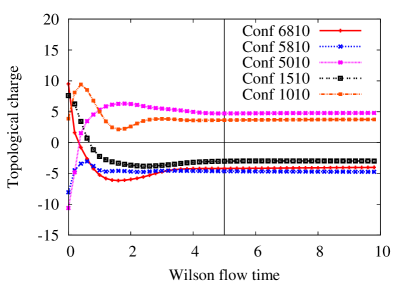
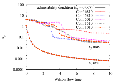
Figure 1: Wilson flow history of the topological charge $Q$ (left panel), and the average and maximum of $s_{p}$ (right) for typical 5 configurations generated at $\beta=4.17$, $m_{\rm ud}=0.007$, and $m_{s}=0.030$. At the flow time of $t=5$ ($\sim 1.4t_{0}$), the topological charge is well saturated.

4 Preliminary results

First, we compute the topological charge density correlator $\langle q(x)q(0)\rangle$ at the Wilson flow time $t_{\rm ref}$ as a function of $|x|=\sqrt{x^{2}}$. Different points giving the same $|x|$ are averaged. The left panel of Fig. 2 shows the data from the $\beta=4.17$ runs. The correlator has a positive core in the short distance region, and goes to negative in the intermediate region, and comes back to around zero. We find saturation (to zero) around $|x|=$1.5–2 fm. We therefore set $r_{\rm cut}=1.6$ fm as the truncation length for the topological susceptibility calculated using Eq. (5).

By also measuring $Q=\sum_{x}q(x)$, we divide the data into topological sectors and check their $Q^{2}$ dependence at long distances, which is predicted in Eq. (4). The right panel of Fig. 2 shows its average in the range $r_{\rm cut}<|x|<L$. Note that the data at $x_{\mu}>L/2$ for any $\mu$ are not averaged to avoid possible effects of the boundary. The expected dependence $Q^{2}/V^{2}$ is clearly seen. We emphasize that this quadratic function has no free parameter to tune. In this plot, we also draw curves whose intercept is given by $\bar{\chi_{t}}$ determined below.

We are now ready for computing $\bar{\chi_{t}}$ in Eq. (5). Note that for our choice $r_{\rm cut}=$ 1.6 fm, $V_{sub}/V\sim$30 %. Namely, the instanton-like lump has enough space, 70% of the whole volume, to escape. Here again the data at $x_{\mu}>L/2$ for any $\mu$ are not averaged to avoid the effect of the boundary. As Fig. 4 shows, the Monte Carlo history of $\bar{\chi_{t}}$ (right panels) fluctuates more frequently than the global topological charge (left panels). In the same panel, we also plot $\bar{\chi_{t}}$ without the correction term from the global topological charge, which apparently shows a stronger correlation with the global topological charge. Namely, this term plays the expected role of canceling the bias from the global topology.

Moreover, as shown in Fig. 4, we find that the sea quark mass dependence of $\bar{\chi_{t}}$ agrees well with the prediction from chiral perturbation theory,

$$\chi_{t}^{\rm ChPT}=\frac{\Sigma}{1/m_{u}+1/m_{d}+1/m_{s}},$$ (7)

where $\Sigma$ denotes the chiral condensate. We can even estimate the (bare) value of chiral condensate as $\Sigma=(250\;\mbox{MeV})^{3}$. Our definition $\bar{\chi_{t}}$ on the configurations generated by the Möbius domain-wall fermions seems to correctly reflect the sea quark’s effect. This implies that the topological fluctuation in our ensembles is just as expected from the effective theory approach. It should be noted that $\bar{\chi}_{t}$ is constructed purely from gluonic quantities. The fermion loop effect is clearly visible in the gauge sector, thanks to the clean signal after the Wilson flow and to the good chiral symmetry of the Möbius domain-wall fermion.

Numerical simulations are performed on IBM System Blue Gene Solution at KEK under a support of its Large Scale Simulation Program (Nos. 12/13-04 and 13/14-04). This work is supported in part by the Grand-in-Aid of the Japanese Ministry of Education (No.25800147, 26400259 26247043), the Grant-in-Aid for Scientific Research (B) (No. 25287046), and SPIRE (Strategic Program for Innovative Research) Field 5.

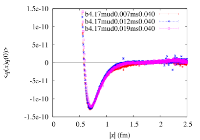
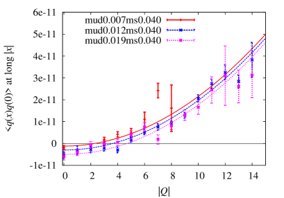
Figure 2: Topological charge density correlator (left panel) and its $|Q|$-dependence (right) in the long distance region $r_{\rm cut}<|x|<L$ at $\beta=4.17$.

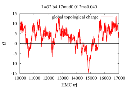
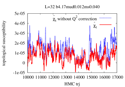
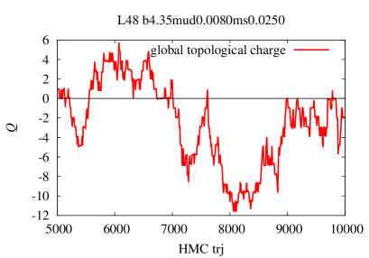
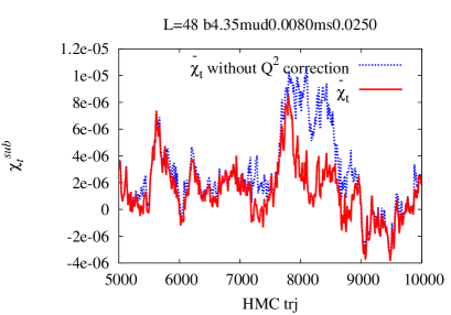
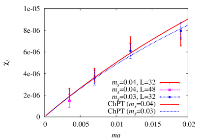
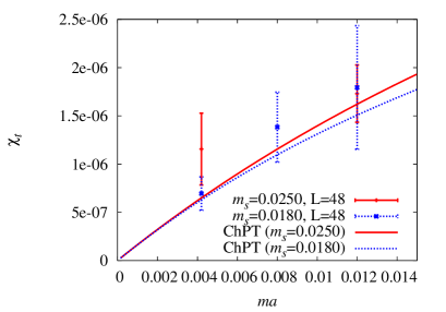
Figure 3: Monte Carlo history (solid lines) of the global topological charge (left) and our new definition of the topological susceptibility $\bar{\chi}_{t}$ (right) at $\beta=4.17,m_{ud}=0.012,m_{s}=0.040$ (top) and $\beta=4.35,m_{ud}=0.0080,m_{s}=0.0250$ (bottom). We also plot $\bar{\chi}_{t}$ without the $Q^{2}/V$ correction term (dotted lines).

Figure 4: The $m_{ud}$ dependence of $\bar{\chi}_{t}$ at $\beta=4.17$ (left) and $\beta=4.35$. For a comparison, we draw the ChPT prediction $\chi_{t}^{\rm ChPT}$ with an input of the chiral condensate $\Sigma=(250\;\mbox{MeV})^{3}$.

References

- [1] S. Schaefer et al. [ALPHA Collaboration], Nucl. Phys. B 845, 93 (2011).
- [2] M. Bruno et al. [ALPHA Collaboration], JHEP 1408, 150 (2014).
- [3] S. Aoki et al. [JLQCD and TWQCD Collaborations], Phys. Lett. B 665, 294 (2008).
- [4] T. W. Chiu et al. [JLQCD and TWQCD Collaborations], PoS LATTICE 2008, 072 (2008).
- [5] G. Cossu et al. [JLQCD Collaboration], Phys. Rev. D 87, no. 11, 114514 (2013).
- [6] H. Fukaya et al. [JLQCD Collaboration], Phys. Rev. D 74, 094505 (2006) [hep-lat/0607020].
- [7] T. Kaneko et al. [The JLQCD Collaboration], PoS LATTICE 2013, 125 (2013).
- [8] R. C. Brower, H. Neff and K. Orginos, Nucl. Phys. Proc. Suppl. 140, 686 (2005); R. C. Brower, H. Neff and K. Orginos, arXiv:1206.5214 [hep-lat].
- [9] R. Brower, S. Chandrasekharan, J. W. Negele and U. J. Wiese, Phys. Lett. B 560, 64 (2003).
- [10] S. Aoki, H. Fukaya, S. Hashimoto and T. Onogi, Phys. Rev. D 76, 054508 (2007).
- [11] P. de Forcrand, M. Garcia Perez, J. E. Hetrick, E. Laermann, J. F. Lagae and I. O. Stamatescu, Nucl. Phys. Proc. Suppl. 73, 578 (1999).
- [12] R. C. Brower et al. [LSD Collaboration], Phys. Rev. D 90, 014503 (2014).
- [13] M. Luscher, JHEP 1008, 071 (2010).
- [14] G. McGlynn and R. D. Mawhinney, Phys. Rev. D 90, 074502 (2014).