Training Design and Channel Estimation in Uplink Cloud Radio Access Networks

Abstract

To decrease the training overhead and improve the channel estimation accuracy under time-varying environments in uplink cloud radio access networks (C-RANs), a superimposed-segment training design is proposed whose core idea is that each mobile station puts a periodic training sequence on the top of the data signal, and remote radio heads (RRHs) insert a separate pilot prior to the received signal before forwarding to the centralized base band unit (BBU) pool. Moreover, a complex-exponential basis-expansion-model (CE-BEM) based maximum a posteriori probability (MAP) channel estimation algorithm is developed, where the BEM coefficients of access links (ALs) and the channel fading of wireless backhaul links (BLs) are first obtained, after which the time-domain channel samples of ALs are restored in terms of maximizing the average effective signal-to-noise ratio (AESNR). Simulation results show that the proposed channel estimation algorithm can effectively decrease the estimation mean square error and increase the AESNR in C-RANs, thus significantly outperforming the existing solutions.

I Introduction

Cloud radio access networks (C-RANs) have received considerable research interest as one of the most promising solutions to mitigate interference, fulfil energy efficiency demands and support high-rate transmission in the fifth generation cellular network [1]. In C-RANs, a large number of remote radio heads (RRHs) are deployed, which operate as non-regenerative relays to forward received signals from mobile stations (MSs) to the centralized base band unit (BBU) pool through wire/wireless backhaul links for uplink transmission [2]. To suppress the inter-RRH interference by using cooperative processing techniques at the BBU pool, the channel state information (CSI) of both the radio access links (ALs) and wireless backhaul links (BLs) are required[3]. In [4], though a segment-training scheme was proposed to estimate the individual channel coefficients for two-hop scenario under flat fading environments, this proposal results in high overhead consumption for backhaul transmission since the RRHs need to forward both AL and BL training sequences to the BBU pool [5]. On the other hand, the superimposed-training scheme [6], where a training sequence is superimposed on the data signal, can significantly reduce the overhead and is valid to perform channel estimation for time-varying environments using complex-exponential basis expansion model (CE-BEM) [7]. However, straightforward implementation of superimposed training in C-RANs would degrade transmission quality due to the fact that superimposing both AL and BL training sequences on the data signal declines the effective signal-to-noise ratio (SNR) [8].

Motivated to reduce the training overhead and enhance the channel estimation performance at the BBU pool, a superimposed-segment training design is proposed in this letter, where superimposed-training is implemented for the radio AL while the segment-training is applied for the wireless BL. Moreover, based on the training design, a CE-BEM based maximum a posteriori probability (MAP) channel estimation algorithm is developed, where the BEM coefficients of the time-varying radio AL and the channel fading of the quasi-static wireless BL are first obtained, after which the time-domain channel samples of the radio AL are restored in terms of maximizing the average effective SNR.

Notation: The transpose, Hermitian and inverse of a matrix are denoted by $\left(\cdot\right)^{T}$, $\left(\cdot\right)^{H}$ and $\left(\cdot\right)^{-1}$, respectively; $\|\cdot\|$ represents the two-norm of a vector; $|\cdot|$ defines the magnitude of a complex argument; $\otimes$ is the Kronecker product; $\mathrm{diag}\left(a_{1},a_{2},\ldots,a_{M}\right)$ denotes the diagonal matrix with $a_{m}$ being the $m$th diagonal element; $\mathrm{tr}\left(\cdot\right)$ represents the trace of a matrix; $\mathbf{I}_{N}$ and $\mathbf{0}_{N}$ are the $N\times N$ unit diagonal matrix and zero matrix, respectively; $\mathbf{1}_{N}$ stands for the $N\times 1$ vector with each entry being unit value; $\mathcal{E}\{\cdot\}$ denotes the expectation of a random variable, and $\hat{x}$ represents its estimate.

II System Model and Training Design

Consider a C-RAN consisting of one BBU pool and multiple RRHs depicted in Fig. 1. The RRHs operate in half-duplex modes, and different MSs served by the same RRU are allocated with a single subcarrier through the orthogonal frequency division multiplexing access (OFDMA) technique. It is assumed that MSs move continuously, while RRUs remain fixed. Thus, the channels of radio ALs would vary during one transmission block, while those of wireless BLs undergo quasi-static flat fading. Due to the orthogonality characteristics of OFDMA for the accessing of multiple MSs, we can focus on the transmission of only a single MS. Let $\mathbf{b}$ and $\mathbf{t}_{s}$ denote the data vector and cyclical training sequence transmitted from the MS, respectively. The training sequence from the RRH is denoted by $\mathbf{t}_{r}$. The $n$-th channel sample of the time-varying radio AL is denoted by $h\!\left(n\right)$ with mean zero and variance $\upsilon_{h}$, while the channel fading of the quasi-static flat BL is denoted by $g$ which has the complex Gaussian distribution of mean zero and variance $\upsilon_{g}$. The transmit power of the MS and RRH are denoted by $P_{s}$ and $P_{r}$, respectively. The noise variance at the RRH and BBU pool is denoted by $\sigma_{n}^{2}$. It is assumed that the BBU pool acquires the knowledge of $\mathbf{t}_{s}$, $\mathbf{t}_{r}$, $\upsilon_{h}$, $\upsilon_{g}$, $P_{s}$, $P_{r}$, and $\sigma_{n}^{2}$.

During each transmission block, the MS transmits a signal $\mathbf{s}$ of $N_{s}$ symbol length to the RRU, in which the $n$-th entry of $\mathbf{s}$ is given by

$$s\!\left(n\right)\!=\!\sqrt{1\!-\!\epsilon}b\!\left(n\right)\!+\!\sqrt{\epsilon}t_{s}\!\left(n\right),\quad 0\!\leq\!n\!\leq\!\left(N_{s}\!-\!1\right),$$ (1)

where $b\!\left(n\right)$ denotes the $n$-th entry of $\mathbf{b}$ with M-ary phase shift keying (MPSK) modulation constrained by $\mathcal{E}\!\big{\{}|b\!\left(n\right)|^{2}\!\big{\}}\!\!=\!\!P_{s}$, and $t_{s}\!\left(n\right)$ represents the $n$-th entry of $\mathbf{t}_{s}$ with $|t_{s}\!\left(n\right)\!|^{2}\!\!=\!\!P_{s}$ whose period is denoted by $N_{p}$. The $\epsilon$ is within $0\!<\!\epsilon\!<\!1$. Without loss of generality, we further assume that $K\!=\!\frac{N_{s}}{N_{p}}$ is an integer[7]. The $n$-th observation at the RRH is written as

$$x_{R}\!\left(n\right)\!=\!h\!\left(n\right)s\!\left(n\right)\!+\!w_{R}\!\left(n\right),\quad 0\!\leq\!n\!\leq\!\left(N_{s}\!-\!1\right),$$ (2)

where $w_{\!R}\!\left(n\right)$ is additive white Gaussian noise (AWGN) at the RRH. Then the RRH scales the received signal by $\alpha\!\!=\!\!\sqrt{\frac{P_{r}}{\upsilon_{h}P_{s}\!+\!\sigma_{n}^{2}}}$, and inserts $\mathbf{t}_{r}$ prior to the received signal. The sequence $\mathbf{t}_{r}$ is of $N_{r}$ length and its $n$-th entry satisfies $|t_{r}\!\left(n\right)\!|^{2}\!\!=\!\!P_{r}$. The BBU pool receives two separate signals as

$$\mathbf{x}_{s}\! =\!\alpha g\cdot\mathrm{diag}\!\left(\mathbf{h}\right)\cdot\mathbf{s}\!+\!\alpha g\mathbf{w}_{R}\!+\!\mathbf{w}_{Ds},$$ (3)

$$\mathbf{x}_{r}\! =\!g\mathbf{t}_{r}\!+\!\mathbf{w}_{Dr},$$ (4)

where $\mathbf{w}_{\!R}\!\!\!=\!\!\!\left[w_{\!R}\!\left(1\right)\ldots w_{\!R}\!\left(\!N_{s}\right)\right]^{T}$, $\mathbf{w}_{\!Ds}\!\!\!=\!\!\!\left[w_{\!Ds}\!\left(1\right)\ldots w_{\!Ds}\!\left(N_{s}\right)\right]^{T}$ and $\mathbf{w}_{\!Dr}\!\!=\!\!\left[w_{Dr}\!\left(1\right),\ldots,w_{Dr}\!\left(N_{r}\right)\right]^{T}$ are AWGN vectors with each entry having variance $\sigma_{n}^{2}$. In order to perform coherent reception and adopt cooperative processing techniques at the BBU pool, the knowledge of $h\!\left(n\right)$’s and $g$ should be obtained, which is explained in the following section.

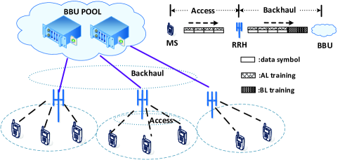
Figure 1: System model and the superimposed-segment training design.

III CE-BEM Based MAP Channel Estimation Algorithm

The CE-BEM for time-selective but frequency-flat fading channels in [9][10] is chosen to model the time-varying AL as

$$h\!\left(n\right)\!=\!\sum_{q\!=\!-Q}^{Q}\!\lambda_{q}e^{j\frac{2\pi qn}{N_{s}}},\quad 0\!\leq\!n\!\leq\!\left(N_{s}\!-\!1\right),$$ (5)

where $\lambda_{q}$’s are the BEM coefficients that remain invariant within one transmission block, and $\lambda_{q}$ has the complex Gaussian distribution with mean zero and variance $\upsilon_{q}$ constrained to $\sum_{q\!=\!-Q}^{Q}\upsilon_{q}\!=\!\upsilon_{h}$. Substituting (5) into (3), $\mathbf{x}_{r}$ can be rewritten as

$$\mathbf{x}_{s}\!=\!\alpha g\mathbf{D}\left[\mathbf{I}_{2Q\!+\!1}\!\otimes\!\mathbf{s}\right]\boldsymbol{\lambda}\!+\!\alpha g\mathbf{w}_{R}\!+\!\mathbf{w}_{Ds},$$ (6)

where $\mathbf{D}\!\!=\!\!\big{[}\mathbf{D}_{-Q},\ldots,\mathbf{D}_{Q}\big{]}$ is an $N_{s}\!\times\!\left(2Q\!+\!1\right)N_{s}$ dimensional matrix with $\mathbf{D}_{q}\!\!=\!\!\mathrm{diag}\!\left(1,e^{j\frac{2\pi q}{N_{s}}},\ldots,e^{j\frac{2\pi q\left(N_{s}\!-\!1\right)}{N_{s}}}\right)$. By defining $\mathbf{J}\!=\!\frac{1}{K}\!\mathbf{1}_{K}^{T}\!\otimes\!\mathbf{I}_{N_{p}}$ of $N_{p}\!\times\!N_{s}$ dimension, we can obtain

$$\mathbf{J}\mathbf{D}_{q}\mathbf{t}_{s}\!=\! \mathbf{\tilde{t}}_{s}, q=0$$ , (7a)

$$\mathbf{J}\mathbf{D}_{q}\mathbf{t}_{s}\!=\! 0, q\neq 0$$ , (7b)

where $\mathbf{\tilde{t}}_{s}$ is an $N_{p}\times 1$ dimensional vector. Left multiplying $\mathbf{x}_{s}$ by $\left(\mathbf{I}_{Q\!+\!1}\!\otimes\!\mathbf{J}\right)\!\mathbf{D}^{H}$ yields

$$\mathbf{r}\!=\!\left(\mathbf{I}_{Q\!+\!1}\!\otimes\!\mathbf{J}\right)\!\mathbf{D}^{H}\mathbf{x}_{s},$$ (8)

whose $\left[\left(q\!+\!Q\right)\!N_{p}\!+\!1\right]$-th to $\left[\left(q\!+\!Q\!+\!1\right)N_{p}\right]$-th entries denoted by $\mathbf{r}_{q}$ can be expressed as

$$\mathbf{r}_{q}\!=\!\alpha g\mathbf{\tilde{t}}_{s}\lambda_{q}\!+\!\underbrace{\alpha g\!\!\!\sum_{l=-Q}^{Q}\!\mathbf{J}\mathbf{D}_{l\!-\!q}\mathbf{b}\lambda_{l}\!+\!\mathbf{J}\mathbf{D}_{q}^{H}\left(\alpha g\mathbf{w}_{R}\!\!+\!\!\mathbf{w}_{Ds}\right)}_{\mathbf{w}_{q}}.$$ (9)

It is testified that

$$\mathcal{E}\!\big{\{}\mathbf{w}_{q1}\mathbf{w}_{q1}^{H}\big{\}}\!=\!\upsilon_{n}\mathbf{I}_{N_{p}},\quad\mathcal{E}\!\big{\{}\mathbf{w}_{q1}\mathbf{w}_{q2}^{H}\big{\}}\!=\!\mathbf{0}_{N_{p}}$$ (10)

for $q_{1}\neq q_{2}$ with $\upsilon_{n}\!\!=\!\!\frac{\alpha^{2}\upsilon_{g}\!\upsilon_{h}\!\left(1\!-\!\epsilon\right)\!P_{s}\!+\!\left(\alpha^{2}\upsilon_{g}\!+\!1\right)\!\sigma_{n}^{2}}{K}$. Although $\mathbf{w}_{q}$ is not a Gaussian vector, it is effective to use the Gaussian distribution to model the noise behavior for estimation problems [14]. Thus, we choose the following function to be the nominal likelihood function of $\mathbf{r}$ as

$$p\!\left(\mathbf{r}|\boldsymbol{\lambda},\!g\right)\!=\!\!\prod_{q\!=\!-Q}^{Q}\!\left(\!\frac{1}{\pi\upsilon_{n}}\!\right)^{\!\!N_{p}}\!\!\!e^{\!-\!\frac{\|\mathbf{r}_{q}\!-\!\alpha g\lambda_{q}\mathbf{\tilde{t}}_{s}\|^{2}}{\upsilon_{n}}}.$$ (11)

III-A Estimation for $\lambda_{q}$’s and $g$

Defining $\boldsymbol{\theta}\!=\!\left[\lambda_{-Q},\ldots,\lambda_{Q},g\right]^{T}$, the MAP estimation for $\boldsymbol{\theta}$ gives

$$\hat{\boldsymbol{\theta}}\!=\!\arg\max_{\boldsymbol{\theta}}\!\Big{\{}p\!\left(\mathbf{r}|\boldsymbol{\lambda},\!g\right)\!p\!\left(\mathbf{x}_{r}|g\right)\!p\!\left(\boldsymbol{\lambda}\right)p\!\left(g\right)\Big{\}}$$ (12)

$$=\!\arg\min_{\boldsymbol{\theta}}\!\Bigg{\{}\!\underbrace{\sum_{q\!=\!-Q}^{Q}\!\!\!\bigg{\{}\!\frac{\|\mathbf{r}_{q}\!\!-\!\!\alpha g\lambda_{q}\mathbf{\tilde{t}}_{s}\|^{2}}{\upsilon_{n}}\!\!+\!\!{\frac{|\lambda_{q}|^{2}}{\upsilon_{q}}}\!\!\bigg{\}}\!\!+\!\!\frac{\|\mathbf{x}_{r}\!\!-\!\!g\mathbf{t}_{r}\|^{2}}{\sigma_{n}^{2}}\!\!+\!\!\frac{|g|^{2}}{\upsilon_{g}}}_{\mathcal{L}\left(\boldsymbol{\theta}\right)}\!\Bigg{\}},$$

where $p\!\left(\mathbf{x}_{r}|g\right)$, $\!p\!\left(\boldsymbol{\lambda}\right)$ and $p\!\left(g\right)$ are Gaussian distribution functions. With a given $g$, the estimate of $\lambda_{q}$ can be obtained as

$$\hat{\lambda}_{q}\!=\!\frac{\alpha g^{H}\tilde{\mathbf{t}}_{s}^{H}\mathbf{r}_{q}}{\alpha^{2}|g|^{2}\|\mathbf{\tilde{t}}_{s}\|^{2}\!+\!\frac{\upsilon_{n}}{\upsilon_{q}}},\!-\!Q\!\leq\!q\!\leq\!Q.$$ (13)

Substituting (13) into (12), the estimate of $g$ can be obtained from

$$\hat{g}\!=\!\arg\min_{g}\!\!\Bigg{\{}\!\!\underbrace{\frac{\|\mathbf{x}_{r}\!\!-\!\!g\mathbf{t}_{r}\|^{2}}{\sigma_{n}^{2}}\!\!+\!\!\frac{|g|^{2}}{\upsilon_{g}}\!\!-\!\!\frac{\alpha^{2}|g|^{2}\!\!\sum_{q\!=\!-Q}^{Q}\!|\mathbf{t}_{s}^{\!H}\mathbf{r}_{q}|^{2}}{\alpha^{2}\upsilon_{n}\!\|\mathbf{\tilde{t}}_{s}\|^{\!2}|g|^{2}\!\!+\!\!\frac{\upsilon_{n}^{2}}{\upsilon_{q}}}}_{\mathcal{L}\!\left(g\right)}\!\!\Bigg{\}}.$$ (14)

Note that, only the first term in $\mathcal{L}\!\left(g\right)$ relates to the phase of $g$ denoted by $\angle{g}$, and thus the estimate of $\angle{g}$ can be directly estimated from minimizing $\|\mathbf{x}_{r}\!-\!g\mathbf{t}_{r}\|^{2}$ as

$$\widehat{\angle{g}}\!=\!\arg\min\!\Big{\{}\|\mathbf{x}_{r}\!\!-\!\!g\mathbf{t}_{r}\|^{2}\!\Big{\}}\!=\!\angle{\left(\mathbf{t}_{r}^{H}\mathbf{x}_{r}\right)}.$$ (15)

The estimate of $|g|$ must be either a local minima of $\mathcal{L}\!\left(|g|\big{|}\angle{g}\right)$ or at the boundary $|g|\!=\!0$, which can be obtained from solving $\frac{\partial\mathcal{L}\!\left(|g|\big{|}\angle{g}\right)}{\partial|g|}\!=\!0$. Unfortunately, a closed-form expression for $|\hat{g}|$ is hard to derive since $\frac{\partial\mathcal{L}\!\left(|g|\big{|}\angle{g}\right)}{\partial|g|}$ is an $m$($\geq 4$)th-order polynomial of $|g|$, and thus numerical methods such as one dimensional search are needed to compute the value of $\widehat{|g|}$. To reduce the complexity of such approaches, an iterative approach is developed whereby $\hat{g}$ is initialized from

$$\hat{g}\! =\!\arg\max_{g}\Big{\{}\!p\!\left(\mathbf{x}_{r}|g\right)p\!\left(g\right)\!\Big{\}}\!=\!\frac{\mathbf{t}_{r}^{H}\mathbf{x}_{r}}{\|\mathbf{t}_{r}\|^{2}\!+\!\frac{\sigma_{n}^{2}}{\upsilon_{g}}}.$$ (16)

With $\hat{g}$ obtained, $\hat{\lambda}_{q}$’s can be estimated according to (13) with $\hat{g}$ in place of $g$. Then, $\hat{g}$ can be further updated by substituting $\hat{\lambda}_{q}$’s into (15) as

$$\hat{g}\!=\!\frac{\sum_{q\!=\!-Q}^{Q}\!\!\frac{\alpha\hat{\lambda}_{q}^{H}\mathbf{\tilde{t}}_{s}^{H}\mathbf{r}_{q}}{\upsilon_{n}}\!+\!\frac{\mathbf{t}_{r}^{H}\mathbf{x}_{r}}{\sigma_{n}^{2}}}{\sum_{q\!=\!-Q}^{Q}\!\!\frac{\alpha^{2}|\hat{\lambda}_{q}|^{2}\|\mathbf{\tilde{t}}_{s}\|^{2}}{\upsilon_{n}}\!+\!\frac{\|\mathbf{t}_{r}\|^{2}}{\sigma_{n}^{2}}\!+\!\frac{1}{\upsilon_{g}}}.$$ (17)

III-B Restoration for Channel Samples $h\!\left(n\right)$’s

With $\hat{\lambda}_{q}$’s obtained, $\hat{h}\!\left(n\right)$ is restored as

$$\hat{h}\!\left(n\right)\!=\!\sum_{q\!=\!-\!Q}^{Q}\!\Big{\{}\eta_{q}\cdot\hat{\lambda}_{q}e^{j\frac{2\pi qn}{N_{s}}}\Big{\}},\quad 0\!\leq\!n\!\leq\!\left(N_{s}\!-1\right),$$ (18)

where $\eta_{q}$’s are real factors. The vector $\boldsymbol{\eta}$ that maximizes the average effective SNR (AESNR) [11] denoted by $\boldsymbol{\eta}^{*}$ is obtained from

$$\boldsymbol{\eta}^{*}\!\!=\!\!\arg\!\max_{\boldsymbol{\eta}}\!\underbrace{\frac{\mathcal{E}\!\bigg{\{}\mathcal{E}\!\Big{\{}\big{|}\hat{g}\hat{h}\!\left(n\right)\big{|}^{2}\Big{|}\boldsymbol{\lambda},\!g\Big{\}}\bigg{\}}\!\left(1\!-\!\epsilon\right)}{\mathcal{E}\!\bigg{\{}\!\mathcal{E}\!\!\Big{\{}\!\!\big{|}\hat{g}\hat{h}\!\left(n\right)\!\!-\!\!gh\!\left(n\right)\!\!\big{|}^{2}\!\Big{|}\boldsymbol{\lambda},g\Big{\}}\!\!+\!\!\left(\!|g|^{\!2}\!\!+\!\!\frac{1}{\alpha^{\!2}}\right)\!\!\frac{\sigma_{n}^{2}}{P_{s}}\bigg{\}}}\!}_{\bar{\gamma}}.$$ (19)

Define $\phi_{q,n}\!\!=\!\!e^{\!j\frac{2\pi qn}{N_{s}}}$, and denote $\Delta{g}$ and $\Delta{\lambda_{q}}$ to be the estimation error of $g$ and $\lambda_{q}$, respectively. It is obtained that

$$\mathcal{E}\!\Big{\{}\!\big{|}\hat{g}\hat{h}\!\left(n\right)\!\big{|}^{2}\!\Big{|}\boldsymbol{\lambda},\!g\!\Big{\}}\!\!=\!\!|g|^{2}\!\!\!\sum_{q\!=\!-Q}^{Q}\!\!\!\eta_{q}^{2}\!\underbrace{\mathcal{E}\!\Big{\{}\!|\Delta{\!\lambda_{q}}|^{\!2}\!\Big{\}}}_{\delta_{\lambda_{q}}}\!+\!\bigg{|}\!\underbrace{\sum_{q\!=\!-Q}^{Q}\!\!\!\eta_{q}\!\lambda_{q}\phi_{q,n}}_{\tilde{h}\!\left(n\right)}\!\bigg{|}^{2}\!\!\underbrace{\!\mathcal{E}\!\Big{\{}\!|\Delta{g}|^{\!2}\!\Big{\}}}_{\delta_{g}}\!+\!|g|^{2}\!\bigg{|}\!\sum_{q\!=\!-Q}^{Q}\!\!\!\eta_{q}\!\lambda_{q}\phi_{q,n}\!\bigg{|}^{2}\!+\!\mathcal{E}\!\Bigg{\{}\bigg{|}\Delta{g}\!\sum_{q\!=\!-Q}^{Q}\!\eta_{q}\Delta{\!\lambda_{q}}\phi_{q,n}\bigg{|}^{2}\Bigg{\}}.$$ (20)

Note that, $\delta_{\lambda_{q}},\delta_{g}\!\sim\!\mathcal{O}\!\left(\frac{\sigma_{n}^{2}}{P_{s}}\right)$ while the last term in (20) has the order of $\mathcal{O}\!\!\left[\!\left(\frac{\sigma_{n}^{2}}{P_{s}}\right)^{\!2}\!\right]$, thus we remove the last term for high SNR approximation, i.e.,

$$\mathcal{E}\!\Big{\{}\!\big{|}\hat{g}\hat{h}\!\left(n\right)\!\big{|}^{2}\!\Big{|}\boldsymbol{\lambda},\!g\!\Big{\}}\!\!=\!|g|^{2}\!\!\!\sum_{q\!=\!-Q}^{Q}\!\!\!\eta_{q}^{2}\delta_{\lambda_{q}}\!\!+\!\big{|}\tilde{h}\!\left(n\right)\!\!\big{|}^{2}\delta_{g}\!\!+\!\!|g|^{2}\!\big{|}\tilde{h}\!\left(n\right)\!\big{|}^{2}.$$ (21)

Similarly,

$$\mathcal{E}\!\Big{\{}\!\big{|}\hat{g}\hat{h}\!\left(n\right)\!\!-\!\!gh\!\left(n\right)\!\big{|}^{2}\!\Big{|}\boldsymbol{\lambda},\!g\!\Big{\}}\!\!\approx \!|g|^{2}\!\!\!\sum_{q\!=\!-Q}^{Q}\!\!\!\eta_{q}^{2}\delta_{\lambda_{q}}\!\!+\!\big{|}\tilde{h}\!\left(n\right)\!\big{|}^{2}\delta_{g}\!\!+\!\!|g|^{2}\!\bigg{|}\!\sum_{q\!=\!-Q}^{Q}\!\left(\eta_{q}\!\!-\!\!1\right)\!\lambda_{q}\phi_{n,q}\!\bigg{|}^{2}.$$ (22)

Due to the non-linearity of the MAP estimation, it is hard to derive the corresponding MSE expressions in closed forms. Moreover, it is known that the MAP estimation MSEs converge to the Cramér-Rao bound (CRB) [12] when the training length is sufficiently large, and thus it is effective to use the CRBs in the computation of the AESNR as

$$\delta_{\!\lambda_{q}}\!\!=\!\!\mathrm{CRB}_{\!\lambda_{q}}\!\!=\!\!\frac{\upsilon_{n}}{\alpha^{2}|g|^{2}\|\mathbf{\tilde{t}}_{s}\|^{2}},\delta_{g}\!=\!\mathrm{CRB}_{g}\!\!=\!\!\frac{1}{\frac{\alpha^{\!2}\|\boldsymbol{\lambda}\|^{\!2}\|\mathbf{\tilde{t}}_{s}\!\|^{\!2}}{\upsilon_{n}}\!\!+\!\!\frac{\|\mathbf{t}_{r}\|^{2}}{\sigma_{n}^{2}}}.$$ (23)

Substituting the above expressions for $\delta_{\lambda_{q}}$ and $\delta_{g}$ into $\bar{\gamma}$ yields

$$\bar{\gamma}\!=\!\frac{\boldsymbol{\eta}^{T}\mathbf{\Xi}\boldsymbol{\eta}\left(1\!-\!\epsilon\right)}{\boldsymbol{\eta}^{T}\mathbf{\Xi}\boldsymbol{\eta}-2\mathbf{1}^{T}_{2Q\!+\!1}\mathbf{\Upsilon}\boldsymbol{\eta}+C},$$ (24)

where

$$\mathbf{\Upsilon}\!\!=\!\!\frac{\alpha^{2}\upsilon_{g}\|\mathbf{\tilde{t}}_{s}\|^{2}}{\upsilon_{n}}\mathbf{R}_{\lambda}^{2}\!\!+\!\!\frac{\alpha^{2}\upsilon_{g}\!\|\mathbf{\tilde{t}}_{s}\|^{2}}{\upsilon_{n}}\mathrm{tr}\!\big{\{}\!\mathbf{R}_{\lambda}\!\big{\}}\mathbf{R}_{\lambda}\!\!+\!\!\frac{\upsilon_{g}\!\|\mathbf{t}_{r}\|^{2}}{\sigma_{n}^{2}}\mathbf{R}_{\lambda},$$ (25)

$$\mathbf{\Xi}\!\!=\!\!\mathbf{\Upsilon}+\mathbf{R}_{\lambda}\!+\!\left(\upsilon_{h}\!+\!\frac{\upsilon_{n}\|\mathbf{t}_{r}\|^{2}}{\sigma_{n}^{2}\alpha^{2}\|\mathbf{\tilde{t}}_{s}\|^{2}}\right)\mathbf{I}_{2Q\!+\!1},$$ (26)

$$C\!\!=\!\!\mathbf{1}^{T}_{2Q\!+\!1}\mathbf{\Upsilon}\mathbf{1}_{2Q\!+\!1}\!\!+\!\!\left(\upsilon_{g}\!\!+\!\!\frac{1}{\alpha^{2}}\!\right)\!\!\left[\frac{\upsilon_{h}\alpha^{2}\|\mathbf{\tilde{t}}_{s}\|^{2}}{\upsilon_{n}}\!+\!\!\frac{\|\mathbf{t}_{r}\|^{2}}{\sigma_{n}^{2}}\right]\!\frac{\sigma_{n}^{2}}{P_{s}},$$ (27)

and $\mathbf{R}_{\lambda}\!\!=\!\!\mathrm{diag}\!\left(\upsilon_{\!-\!Q}\ldots\upsilon_{Q}\right)$. On setting $\varphi^{*}\!\!=\!\!\left(\boldsymbol{\eta}^{*}\right)^{T}\mathbf{\Xi}\boldsymbol{\eta}^{*}$, the optimization for $\boldsymbol{\eta}$ transforms to

$$\max_{\boldsymbol{\eta}}\quad 2\mathbf{1}^{T}_{2Q\!+\!1}\mathbf{\Upsilon}\boldsymbol{\eta},$$ (28)

$$\mathrm{s.t.}\quad\boldsymbol{\eta}^{T}\mathbf{\Xi}\boldsymbol{\eta}\!=\!\varphi^{*}.$$ (29)

Clearly, the optimization problem described in (28) constrained by (29) is concave, and $\boldsymbol{\eta}^{*}$ can be directly obtained from the Lagrange dual function as

$$\boldsymbol{\eta}^{*}\!=\!\frac{\sqrt{\varphi^{*}}\mathbf{\Xi}^{-1}\mathbf{\Upsilon}\mathbf{1}_{2Q\!+\!1}}{\sqrt{\mathbf{1}_{2Q\!+\!1}^{T}\mathbf{\Upsilon}\mathbf{\Xi}^{-1}\mathbf{\Upsilon}\mathbf{1}_{2Q\!+\!1}}}.$$ (30)

Substituting (30) back to (24), the optimization problem becomes

$$\max_{\varphi}\quad\frac{\varphi}{\varphi-2\sqrt{\mathbf{1}_{2Q\!+\!1}^{T}\mathbf{\Upsilon}\mathbf{\Xi}^{-1}\mathbf{\Upsilon}\mathbf{1}_{2Q\!+\!1}}\sqrt{\varphi}+C},$$ (31)

$$\mathrm{s.t.}\quad\varphi>0,$$ (32)

whose solution is $\varphi^{*}=\frac{C^{2}}{\mathbf{1}_{2Q\!+\!1}^{T}\mathbf{\Upsilon}\mathbf{\Xi}^{-1}\mathbf{\Upsilon}\mathbf{1}_{2Q\!+\!1}}$ leading to

$$\boldsymbol{\eta}^{*}=\frac{C\mathbf{\Xi}^{-1}\mathbf{\Upsilon}\mathbf{1}_{2Q\!+\!1}}{\mathbf{1}_{2Q\!+\!1}^{T}\mathbf{\Upsilon}\mathbf{\Xi}^{-1}\mathbf{\Upsilon}\mathbf{1}_{2Q\!+\!1}}.$$ (33)

Combining the estimation for $\boldsymbol{\theta}$ and the restoration for $h\!\left(n\right)$’s, the proposed channel estimation algorithm is summarized in Table I. Moreover, the following proposition is given to demonstrate the effectiveness of the proposed algorithm:

$\mathbf{Proposition}$ 1

The iterative channel estimation algorithm is convergent, and it achieves lower MSE than that of the maximum likelihood (ML) method.

Proof:

Each iteration consists of $\left(2Q\!+\!2\right)$ steps. Denote the $i$th entry of $\boldsymbol{\theta}$ by $\theta_{i}$, and the updated estimate of $\theta_{i}$ denoted by $\hat{\theta}_{i}^{\mathrm{new}}$ satisfies $\mathcal{L}\!\left(\hat{\theta}_{i}^{\mathrm{new}}\right)\!>\!\mathcal{L}\!\left(\hat{\theta}_{i}\right)$. This indicates that $\mathcal{L}\!\left(\boldsymbol{\theta}\right)$ strictly increases after each step as well as after one round of iteration. It is known that $\mathcal{L}\!\left(\boldsymbol{\theta}\right)$ is continuous with respect to $\theta_{i}$ and $\mathcal{L}\!\left(\boldsymbol{\theta}\right)\!<\!+\infty$. Thus, it is concluded that the iterative algorithm is convergent.

From (13), the MAP estimate of $g$ with a given $\boldsymbol{\lambda}$ is

$$\hat{g}^{\mathrm{MAP}}\!\!\!\!=\!\!\frac{\frac{\alpha^{2}\|\boldsymbol{\lambda}\|^{2}\|\mathbf{\tilde{t}}_{s}\|^{2}}{\upsilon_{n}}\!+\!\frac{\|\mathbf{t}_{r}\|^{2}}{\sigma_{n}^{2}}}{\frac{\alpha^{2}\|\boldsymbol{\lambda}\|^{2}\|\mathbf{\tilde{t}}_{s}\|^{2}}{\upsilon_{n}}\!\!+\!\!\frac{\|\mathbf{t}_{r}\|^{2}}{\sigma_{n}^{2}}\!\!+\!\!\frac{1}{\upsilon_{g}}}g\!+\!\frac{\sum_{q\!=\!-Q}^{Q}\!\!\frac{\alpha\lambda_{q}^{H}\mathbf{\tilde{t}}_{s}^{H}\mathbf{w}_{q}}{\upsilon_{n}}\!\!+\!\!\frac{\mathbf{t}_{r}^{H}\mathbf{w}_{Dr}}{\sigma_{n}^{2}}}{\frac{\alpha^{2}\|\boldsymbol{\lambda}\|^{2}\|\mathbf{\tilde{t}}_{s}\|^{2}}{\upsilon_{n}}\!\!+\!\!\frac{\|\mathbf{t}_{r}\|^{2}}{\sigma_{n}^{2}}\!\!+\!\!\frac{1}{\upsilon_{g}}},$$

whose MSE is calculated as

$$\delta_{g}^{\mathrm{MAP}}\!\!\!\! =\!\mathcal{E}\!\Big{\{}\!\big{\|}\hat{g}^{\mathrm{MAP}}\!\!\!-\!g\big{\|}^{\!2}\!\Big{\}}\!\!$$

$$=\!\!\frac{1}{\frac{\alpha^{\!2}\|\boldsymbol{\lambda}\|^{\!2}\|\mathbf{\tilde{t}}_{s}\|^{\!2}}{\upsilon_{n}}\!\!+\!\!\frac{\|\mathbf{t}_{r}\|^{\!2}}{\sigma_{n}^{2}}}\frac{\upsilon_{g}}{\upsilon_{g}\!\!+\!\!\frac{1}{\frac{\alpha^{\!2}\|\boldsymbol{\lambda}\|^{\!2}\|\mathbf{\tilde{t}}_{s}\|^{\!2}}{\upsilon_{n}}\!+\!\frac{\|\mathbf{t}_{r}\|^{\!2}}{\sigma_{n}^{2}}}}.$$ (34)

The ML estimate of $g$ gives

$$\hat{g}^{\mathrm{ML}}\!\!=\!g\!+\!\frac{\sum_{q\!=\!-Q}^{Q}\!\!\frac{\alpha\lambda_{q}^{H}\mathbf{\tilde{t}}_{s}^{H}\mathbf{w}_{q}}{\upsilon_{n}}\!\!+\!\!\frac{\mathbf{t}_{r}^{H}\mathbf{w}_{Dr}}{\sigma_{n}^{2}}}{\frac{\alpha^{2}\|\boldsymbol{\lambda}\|^{2}\|\mathbf{\tilde{t}}_{s}\|^{2}}{\upsilon_{n}}\!\!+\!\!\frac{\|\mathbf{t}_{r}\|^{2}}{\sigma_{n}^{2}}},$$

whose MSE is calculated as

$$\delta_{g}^{\mathrm{ML}}\! =\!\mathcal{E}\!\Big{\{}\!\big{\|}\hat{g}^{\mathrm{ML}}\!\!\!-\!g\big{\|}^{\!2}\!\Big{\}}\!=\!\frac{1}{\frac{\alpha^{2}\|\boldsymbol{\lambda}\|^{2}\|\mathbf{\tilde{t}}_{s}\|^{2}}{\upsilon_{n}}\!+\!\frac{\|\mathbf{t}_{r}\|^{2}}{\sigma_{n}^{2}}}.$$ (35)

Clearly, $\delta_{g}^{\mathrm{MAP}}\!\!<\!\delta_{g}^{\mathrm{ML}}$ always holds, and it can be also testified that $\delta_{\lambda_{q}}^{\mathrm{MAP}}\!\!<\!\!\delta_{\lambda_{q}}^{\mathrm{ML}}$ is satisfied similarly. ∎

Remark: According to (III-B) and (35), we see that $\delta_{g}^{\mathrm{MAP}}\!\!<\!\!\mathrm{CRB}_{g}$ and $\delta_{g}^{\mathrm{ML}}\!\!=\!\!\mathrm{CRB}_{g}$. This is because the proposed MAP estimation algorithm is biased since $\mathcal{E}\!\{\hat{g}^{\mathrm{MAP}}\!\}\!\!\neq\!\!g$.

TABLE I: Iterative Channel Estimation Algorithm

• Initialize $\hat{g}$ in accordance with (16); i_Index$=$i_Times($>0$) • Repeat - For each $q$, update $\hat{\lambda}_{q}$ by substituting $\hat{g}$ into (13). - Update $\hat{g}$ by substituting $\hat{\lambda}_{q}$’s into (17). - i_Index$=$i_Index$-1$ • Until i_Index$\leq 0$ is satisfied. • Calculate the optimal $\boldsymbol{\eta}^{*}$ according to (33). • Restore $\hat{h}\!\left(n\right)$’s according to (18) by using $\hat{\lambda}_{q}$’s and $\boldsymbol{\eta}^{*}$. • Return $\hat{h}\!\left(n\right)$’s and $\hat{g}$.

IV Numerical Results

Numerical results are provided to evaluate the performance of the CE-BEM based MAP (C-MAP) channel estimation algorithm. The AL channel $\big{\{}\!h\!\left(n\right)\!\!\big{\}}$ and BL channel $g$ are generated from the spatial channel model (CSM) in 3GPP TR 25.996 [13]. The parameters are set as $N_{s}\!=\!800$, $N_{r}\!=\!4$ and $\mathrm{i\_Times}\!\!\!=\!\!\!10$. We assume binary-phase-shift-keying (BPSK) modulation for $\big{\{}\!b\!\left(n\right)\!\!\big{\}}$, while $\mathbf{\tilde{t}}_{s}$ is selected as the $2$nd column of the $N_{p}\!\times\!N_{p}$ discrete Fourier transform (DFT) matrix and $\mathbf{t}_{r}$ is as the $3$rd column of the $N_{r}\!\times\!N_{r}$ DFT matrix. The transmit power $P_{s}$ and $P_{r}$ are set to be equal, and the noise variance is set to be of unit value; thus the SNR is equal to $P_{s}$.

In Fig. 2, the average MSEs of both AL and BL channels for C-MAP estimation are compared with that for ML estimation. It is observed that the proposed C-MAP estimation outperforms the traditional ML method since C-MAP achieves lower MSEs of both AL and BL channels than ML. Moreover, it is seen that the MSE of the AL channel for the ML method is not convergent. This is because random generation of $g$ would result in singularity, e.g., $g\!\!\rightarrow\!\!0$, leading to $\Delta\!\lambda_{q}\!\!\rightarrow\!\!\infty$ for the ML method, while the proposed C-MAP algorithm is robust at the singularity. In Fig.3, we evaluate the AESNR performance for the optimal weighted approach (OWA) to channel restoration. It is seen that OWA obtains higher AESNRs than the baseline (restoring according to CE-BEM), especially in the low SNR region, and it draws near to the baseline as SNR increases.

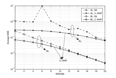
Figure 2: Average MSE versus SNR for different estimation methods.

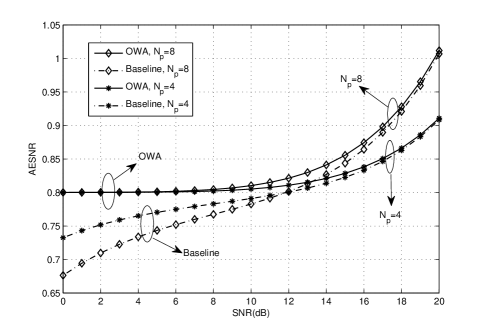
Figure 3: AESNR versus SNR for different channel restoring methods.

V Conclusions

A superimposed-segment training design has been proposed to decrease the training overhead and enhance the channel estimation accuracy in uplink C-RANs. Based on the training design, a CE-BEM based MAP channel estimation algorithm has been developed, where the BEM coefficients of the time-varying radio AL and the channel fading of the quasi-static wireless BL are first obtained, then the time-domain channel samples of AL are restored from maximizing AESNR. Simulation results have demonstrated that the proposed algorithm declines the estimation MSE and increases the AESNR.

References

• [1] C. I, et al., “Toward green and soft: A 5G perspective,”  IEEE Commun. Mag., vol. 52, no. 2, pp. 66–73, Feb. 2014.
• [2] Y. Zhou and W. Yu, “Optimized backhaul compression for uplink cloud radio access network,” IEEE J. Sel. Areas Commun., vol. 32, no. 6, pp. 1295–1307, June 2014.
• [3] S. Park, et al., “Robust layered transmission and compression for distributed uplink reception in cloud radio access networks,” IEEE Trans. Veh. Technol., vol. 63, no. 1, pp. 204–216, Jan. 2014.
• [4] S. Zhang, F. Gao, C. Pei and X. He, “Segment training based individual channel estimation in one-way relay network with power allocation,” IEEE Trans. Wireless Commun., vol. 12, no. 3, pp. 1300–1309, Mar. 2013.
• [5] T. Biermann, et al., “How backhaul networks influence the feasibility of coordinated multipoint in cellular networks,” IEEE Commun. Mag., vol. 51, no. 8, pp. 168–176, Aug. 2013.
• [6] J. Tugnait and W. Luo, “On channel estimation using superimposed training and first-order statistics,” IEEE Commun. Lett., vol. 7, no. 9, pp. 413–416, Sep. 2003.
• [7] G. Giannakis and C. Tepedelenlioglu, “Basis expansion models and diversity techniques for blind identification and equalization of time-varying channels,” Proc. IEEE, vol. 86, pp. 1969–986, Nov. 1998.
• [8] G. Dou, C. He, C. Li and J. Gao, “A weighted first-order statistical method for time-varying channel and DC-offset estimation using superimposed training,” IEEE Commun. Lett., vol. 17, no. 5, pp. 852–855, May 2013.
• [9] X. Ma and G. Giannakis, “Maximum-diversity transmissions over doubly-selective wireless channels,” IEEE Trans. Inf. Theory, vol. 49, pp. 1832–1840, July 2003.
• [10] G. Wang, et al., “Channel estimation and training design for two-way relay networks in time-selective fading environments,” IEEE Trans. Wireless Commun., vol. 10, no. 8, pp. 2681–2691, Aug. 2011.
• [11] F. Gao, R. Zhang and Y. Liang, “Optimal channel estimation and training design for two-way relay networks,” IEEE Trans. Commun., vol. 57, no. 10, pp. 3024–3033, Oct. 2009.
• [12] E. Carvalho, J. Cioffi and D. Slock, “Cramér-rao bounds for blind multichannel estimation,” in Proc. IEEE GLOBECOM, San Francisco, pp. 1036–1040, Nov. 2000.
• [13] “Spatial channel model for multiple input multiple output simulations,” 3GPP TR 25.996, release 9, Dec. 2009.
• [14] S. M. Kay, Fundamentals of Statistical Signal Processing, Volume I: Estimation Theory. Prentice Hall PTR, 1993.
• [15] A. Goldsmith, Wirelss Communications. Cambridge, England: Cambridge University Press, 2005.