Network Cross-Validation for Determining the Number of Communities in Network Data

Abstract

The stochastic block model and its variants have been a popular tool in analyzing large network data with community structures. In this paper we develop an efficient network cross-validation (NCV) approach to determine the number of communities, as well as to choose between the regular stochastic block model and the degree corrected block model. The proposed NCV method is based on a block-wise node-pair splitting technique, combined with an integrated step of community recovery using sub-blocks of the adjacency matrix. We prove that the probability of under selection vanishes as the number of node increases, under mild conditions satisfied by a wide range of popular community recovery algorithms. The solid performance of our method is also demonstrated in extensive simulations and a data example.

1 Introduction

In the last few decades, the amount of network data and the need for relevant statistical inference tools are growing at a rapid pace. One of the main research topics in network data analysis is to identify hidden communities from a single observed network. Roughly speaking, network community refers to the phenomenon that individuals close to each other are more likely to connect, and hence the edge density varies from within coherent subpopulations to between subpopulations (Newman & Girvan, 2004; Newman, 2006). The stochastic block model (Holland et al., 1983) and its variants such as the degree corrected block model (Karrer & Newman, 2011) are powerful and mathematically elegant tools to model large networks with community structures, and have been proved useful in many scientific areas such as social science, biology, and information science (Faust & Wasserman, 1992; Kemp et al., 2006; Bickel & Chen, 2009).

The community recovery problem for stochastic block models has been the focus of much research effort in the past decade, in several areas including statistics (Bickel & Chen, 2009; Zhao et al., 2012; Jin, 2012; Fishkind et al., 2013; Lei & Rinaldo, 2013), machine learning (McSherry, 2001; Chen et al., 2012; Chaudhuri et al., 2012; Anandkumar et al., 2014), statistical physics (Decelle et al., 2011; Krzakala et al., 2013), and probability theory (Massoulie, 2013; Mossel et al., 2013; Abbe et al., 2014). These methods are based on a wide range of different tools such as maximum likelihood, convex optimization, spectral methods, and belief propagation, etc. However, almost all of these methods require $K$, the total number of communities, to be known in advance.

Unlike the community recovery problem, determining the number of communities remains a challenging problem and gains increasing interest recently. Zhao et al. (2011) propose to sequentially extract one significant community from the remaining of the network, and they approximate the null distribution of their optimizing statistic by bootstrapping from an Erdős-Rényi graph. Bickel & Sarkar (2013) propose to test $K=1$ vs $K>1$ at each step of a recursive bipartition algorithm. They derive the asymptotic null distribution of the largest eigenvalue of the suitably scaled and centered adjacency matrix. But the convergence rate is slow and an empirical tuning is needed in practice. Moreover, these sequential or recursive testing procedures only work for certain types of community structures. After the first draft of this work, there have been some new developments along the line of testing $K=\tilde{K}$ for a given candidate value $\tilde{K}$ (Lei, 2014). Some model selection criteria based on approximated likelihood or Bayesian inference have also been proposed, including Latouche et al. (2012); McDaid et al. (2013); Saldana et al. (2014); Wang & Bickel (2015). The performance of these methods often crucially depends on the choice of a penalty term or some prior knowledge of the model parameters.

In this paper, we focus on a generic idea of network cross-validation. Cross-validation is a very popular and appealing method in many model selection problems. The adaptation to network data is usually through a node splitting procedure and has been considered by Airoldi et al. (2008); Neville et al. (2012), among others. A random node-pair splitting method has been used in Hoff (2008) for model selection under a Bayesian framework. These methods, even though applicable to the community recovery problem, are usually computationally intensive. More detailed discussion and comparison can be found in Section 2.1. Moreover, the theoretical investigation for cross-validation methods in network model selection remains open.

The NCV method developed in this paper is based on a block-wise node-pair splitting technique. The splitting step divides the nodes randomly into two groups $\mathcal{N}_{1}$ and $\mathcal{N}_{2}$. The observed edge formation between node pairs $(i,j)$, for $i\in\mathcal{N}_{1}$, and $j\in\mathcal{N}_{1}\cup\mathcal{N}_{2}$ are used as a fitting set, and the node pairs $(i,j)$ for $i,j\in\mathcal{N}_{2}$ are used as a testing set. Such a node-pair splitting is superior to a simple node splitting. It originates from two key observations. First, the fitting set carries substantial relationship information for all nodes in the network. That is, we can consistently estimate the membership of all the nodes as well as the community-wise edge probability matrix from the fitting set. Second, given the community membership, the edge formation in the fitting set and in the testing set are independent. The second observation reflects a significant difference between the traditional parameterization of the stochastic block model that treats the node memberships as missing variables, and the conditional parameterization that treats the memberships as parameters. The traditional parameterization can model networks of arbitrary size and has a motivation from exchangeable random graphs (Bickel & Chen, 2009). However, for community recovery based on a single observed realization of the stochastic block model, the useful information for statistical inference is largely contained in the randomness of edge formation.

We describe the algorithm in detail in Section 2. The proposed V-fold NCV method is novel and is of substantial practical interest for several reasons. First, it is computationally efficient, requiring only one model fitting for each fold. Second, it is tuning free except the number of folds. Moreover, it is general enough to be combined with different community recovery techniques. In Section 2.5, we characterize the theoretical properties of the proposed NCV method. We show that under appropriate conditions, when combined with popular community recovery techniques, such as modularity based optimization and spectral clustering, the proposed NCV does not underestimate the number of communities with probability tending to one. The protection against overestimating is also discussed. In Section 4, we demonstrate the effectiveness of our method via extensive simulations, where different types of network community structures are investigated.

The NCV method can be applied to select the best model from a general collection of candidate models, which does not need to be nested or hierarchical. For example, one can use NCV to choose between the regular stochastic block model and the degree corrected block model, with simultaneous choice of number of communities. Moreover, the block-wise node-pair splitting idea behind NCV can be further extended to other network models with conditional edge independence. These extensions are described in Section 3 and Section 5, and illustrated in an application to a political blog data in Section 4, where the NCV method chooses the degree corrected block model with two communities, matching pervious findings in the literature. Further discussions can be found in Section 5.

2 Network cross-validation for stochastic block models

In a stochastic block model with $n$ nodes and $K$ communities, the observed random graph is often represented by a $n$ by $n$ symmetric binary adjacency matrix $A$. The community structure is represented by a vector $g\in\{1,...,K\}^{n}$ with $g_{i}$ being the community that node $i$ belongs to. Given the membership vector $g$, each edge $A_{ij}$ ($i<j$) is an independent Bernoulli variable satisfying

$$P(A_{ij}=1)=1-P(A_{ij}=0)=B_{g_{i}g_{j}}\,,$$ (1)

where $B\in[0,1]^{K\times K}$ is a symmetric matrix representing the community-wise edge probability. In this section we focus on the problem of estimating $K$, the number of communities, from a single observed network $A$. Generalization to other model selection problems is straightforward and will be discussed in later sections.

2.1 Block-wise node-pair splitting

Let $(\mathcal{N}_{1},\mathcal{N}_{2})$ be a random partition of the nodes, the adjacency matrix can be written in a block form

$$A=\left(\begin{array}[]{cc}A^{(11)}&A^{(12)}\\ A^{(21)}&A^{(22)}\end{array}\right)\,,$$ (2)

where $A^{(jj)}$ is the adjacency matrix for nodes in $\mathcal{N}_{j}$ ($j=1,2$). The splitting step puts node pairs in $A^{(11)}$ and $A^{(12)}$ in the fitting sample and puts node pairs in $A^{(22)}$ in the testing sample. Such a split makes full use of the entire observed adjacency matrix and provides a way to directly compare multiple candidate values of $K$ based on the predictive loss on the testing sample.

The block-wise node-pair splitting is novel, and has several appealing features when compared with existing cross-validation methods for network data that are mostly based on a node splitting technique. In the node splitting method, where the nodes, instead of the node pairs, are split into a fitting set and a testing set, one typically uses the parameterization of the membership distribution $\pi=(\pi_{1},...,\pi_{K})$ such that the node membership is generated independently with probability $P(g_{i}=k)=\pi_{k}$ for $1\leq i\leq n$. After the node splitting, the model parameter $(\pi,B)$ is estimated on the subnetwork confined on the fitting set of nodes, and evaluated on the subnetwork confined on the testing subset of nodes. This approach has some drawbacks. First, calculating the full likelihood in terms of $\pi$ and $B$ in presence of a missing membership vector $g$ is computationally demanding. Second, it does not use the observed edge formation between the fitting and testing nodes, introducing unnecessary randomness in the validation step by treating the node memberships as random variables. In contrast, the block-wise node-pair splitting allows us to use the conditional parameterization that treats the memberships as parameters and estimate, from the fitting set of node pairs, the membership $g$ for all nodes in the entire network. Such a procedure fully exploits the information carried in node pairs between $\mathcal{N}_{1}$ and $\mathcal{N}_{2}$, making the model fitting and validation statistically and computationally more efficient.

Comparing with the uniformly random node-pair splitting method, the proposed block-wise splitting technique is much simpler to implement as many existing community recovery methods can be easily extended to the rectangular adjacency matrix $(A^{(11)},A^{(12)})$ (Section 2.2). In contrast, the random node-pair splitting will result in incomplete adjacency matrices, and users are left with limited choices which are mainly based on likelihood.

2.2 Estimating model parameters from the rectangular matrix

After splitting, we estimate model parameters $(g,B)$ from the $n_{1}\times n$ rectangular matrix $A^{(1)}=(A^{(11)},A^{(12)})$, where $n_{1}$ is the cardinality of $\mathcal{N}_{1}$. Many standard procedures designed for the full adjacency matrix can be extended to this case, such as likelihood based methods and spectral methods. Here we focus on spectral clustering, because it is simple to implement and the analysis is straightforward. This is also the method we implement in the numerical experiments presented in Section 4.

For a given candidate value $\tilde{K}$ of $K$, the simple spectral clustering method first performs a singular value decomposition on $A^{(1)}$, and estimates $g$ by applying $k$-means clustering on the rows of the $n\times\tilde{K}$ matrix consisting of the leading $\tilde{K}$ right singular vectors. Once $\hat{g}$ is obtained, let $\mathcal{N}_{j,k}$ be the nodes in $\mathcal{N}_{j}$ with estimated membership $k$, and $n_{j,k}=|\mathcal{N}_{j,k}|$ ($j=1,2$, $1\leq k\leq\tilde{K}$). We can estimate $B$ using a simple plug-in estimator:

$$\hat{B}_{k,k^{\prime}}=\left\{\begin{array}[]{ll}{\displaystyle\frac{\sum_{i\in\mathcal{N}_{1,k},j\in\mathcal{N}_{1,k^{\prime}}\cup\mathcal{N}_{2,k^{\prime}}}A_{ij}}{n_{1,k}(n_{1,k^{\prime}}+n_{2,k^{\prime}})}}\,,&k\neq k^{\prime}\,,\\ &\\ {\displaystyle\frac{\sum_{i,j\in\mathcal{N}_{1,k},i<j}A_{ij}+\sum_{i\in\mathcal{N}_{1,k},j\in\mathcal{N}_{2,k}}A_{ij}}{(n_{1,k}-1)n_{1,k}/2+n_{1,k}n_{2,k}}}\,,&k=k^{\prime}\,.\end{array}\right.$$ (3)

2.3 Validation using the testing set

After estimating the parameters $(\hat{g},\hat{B})$, we can assess the goodness-of-fit by validating on the testing set.

For each observation in the testing set, $A_{ij}$ ($i\neq j$, $i,j\in\mathcal{N}_{2}$) is a Bernoulli random variable with parameter $P_{ij}=B_{g_{i}g_{j}}$, which is estimated by $\hat{P}_{ij}=\hat{B}_{\hat{g}_{i}\hat{g}_{j}}$. Some natural choices of the loss function $\ell$ include negative log-likelihood $\ell(x,p)=-x\log p-(1-x)\log(1-p)$, and squared error $\ell(x,p)=(x-p)^{2}$. In our numerical experiments, these two loss functions give almost identical performance.

In the validation step, if the candidate value $\tilde{K}$ is too small, then the fitted model cannot capture the fine structures in the data, and will likely lead to poor predictive loss on testing data. If $\tilde{K}$ is too large, then the model over fits the data, with noisy prediction on the testing data. Therefore, it is natural to expect the validated predictive loss $\hat{L}(A,\tilde{K})=\sum_{i,j\in\mathcal{N}_{2},i\neq j}\ell(A_{ij},\hat{P}_{ij})\,,$ to be minimized when $\tilde{K}=K$, the true number of communities. Partial theoretical supports and further heuristic arguments are given in Section 2.5.

2.4 V-fold network cross-validation

Now we formally describe the V-fold network cross-validation procedure.

Algorithm 1: V-fold network cross-validation

1. Input: adjacency matrix $A$, a set $\mathcal{K}$ of candidate values for $K$, number of folds $V\geq 2$.

2. Randomly split the adjacency matrix into $V\times V$ equal sized blocks

   $$A=(A^{(uv)}:1\leq u,v\leq V)$$

   similarly as in (2), where the nodes are partitioned into $V$ equal-sized subsets $\mathcal{N}_{v}$ ($1\leq v\leq V$); $A^{(vv)}$ contains observation between node pairs in the $v$th random subset $\mathcal{N}_{v}$; and $A^{(uv)}$ contains observation between $\mathcal{N}_{v}$ and $\mathcal{N}_{v}$.

3. For each $1\leq v\leq V$, and each $\tilde{K}\in\mathcal{K}$

   1. Estimate model parameters $(\hat{g}^{(v)},\hat{B}^{(v)})$ using the rectangular submatrix obtained by removing the rows of $A$ in subset $\mathcal{N}_{v}$

      $$A^{(-v)}=(A^{(rs)}:r\neq v,\ 1\leq r,s\leq V)\,.$$

   2. Calculate the predictive loss evaluated on $A^{(vv)}$:

      $$\hat{L}^{(v)}(A,\tilde{K})=\sum_{i,j\in\mathcal{N}_{v},i\neq j}\ell(A_{ij},\hat{P}^{(v)}_{ij})\,,$$

      where $\hat{P}^{(v)}_{ij}=\hat{B}^{(v)}_{\hat{g}^{(v)}_{i},\hat{g}^{(v)}_{j}}$.

4. Let $\hat{L}(A,\tilde{K})=\sum_{v=1}^{V}\hat{L}^{(v)}(A,\tilde{K})$ and output

   $$\hat{K}=\arg\min_{\tilde{K}\in\mathcal{K}}\hat{L}(A,\tilde{K})\,.$$

In our experiments we found the performance of NCV insensitive to the choice of $V$, and we used $V=3$ for all numerical experiments. Further discussion on the choice of $V$ and its difference from the regular cross-validation is given in Section 5.

2.5 Theoretical properties

For two sequences $a_{n}$ and $b_{n}$, we denote $a_{n}=\Omega(b_{n})$ if $b_{n}=O(a_{n})$, and $a_{n}=\omega(b_{n})$ if $b_{n}=o(a_{n})$.

To study the asymptotic behavior of the estimator, we consider a sequence of SBM’s parameterized by $(g^{(n)},B^{(n)}:n\geq 1)$ such that

1. $g^{(n)}$ is a membership vector of length $n$ with $K$ distinct communities, and the minimum block size is at least $\pi_{0}n$ for some constant $\pi_{0}$.

2. $B^{(n)}=\rho_{n}B_{0}$ where $B_{0}$ is a $K\times K$ symmetric matrix with entries in $(0,1]$, and the rows of $B_{0}$ are all distinct. The rate $\rho_{n}$ controls the largest edge probability and satisfies $\rho_{n}=\Omega(\log n/n)$.

The first condition requires the block sizes to be relatively balanced. It is satisfied with high probability if the memberships are independently generated from a multinomial distribution. The second condition allows the edge probability to decrease at a rate $\rho_{n}$ as $n$ increases. The lower bound on the sparsity $\rho_{n}$ makes it possible to obtain accurate community recovery.

The community recovery is an integrated part in the proposed NCV method and its accuracy plays an important role in the performance of model selection. We introduce two notions of community recovery consistency.

Definition 1 (Exactly consistent recovery).

Given a sequence of SBM’s with $K$ blocks parameterized by $(g^{(n)},B^{(n)})$, we call a community recovery method $\hat{g}$ exactly consistent if $P(\hat{g}(A,K)=g^{(n)})\rightarrow 1$, where $A$ is a realization of SBM $(g^{(n)},B^{(n)})$ and the equality is up to a possible label permutation.

Definition 2 (Approximately consistent recovery).

For a sequence of SBM’s with $K$ blocks parameterized by $(g^{(n)},B^{(n)})$ and a sequence $\eta_{n}=o(1)$, we say $\hat{g}$ is approximately consistent with rate $\eta_{n}$ if,

$$\lim_{n\rightarrow\infty}P[{\rm Ham}(\hat{g}(A,K),g)\geq\eta_{n}n]=0,$$

where ${\rm Ham}(\hat{g},g)$ is the smallest Hamming distance between $\hat{g}$ and $g$ among all possible label permutations.

Exactly consistent community recovery can be achieved under mild assumptions on $g^{(n)}$ and $B^{(n)}$. It is known that likelihood methods (Bickel & Chen, 2009) are exactly consistent when $\rho_{n}n/\log n\rightarrow\infty$, and variants of spectral methods (McSherry, 2001; Vu, 2014; Lei & Zhu, 2014) are exactly consistent when $\rho_{n}n/\log n>C$ for some constant $C$ depending on $\pi_{0}$, $B_{0}$ only. For the simple spectral clustering algorithm used in our numerical study, the exact consistency result has not been established. In the following, we first establish the approximately consistent recovery result when $K$ is the true number of blocks.

Theorem 1 (Consistency of spectral clustering).

Under assumptions A1–A2, for each fold split in NCV, the $\hat{g}$ estimated using spectral clustering as described in Section 2.2 is approximately consistent with rate $(n\rho_{n})^{-1}$.

Now we state the main theorem. For a given $V$-fold block-wise partition of $A$, Let

$$L(A)=\sum_{v=1}^{V}\sum_{i,j\in\mathcal{N}_{v},i\neq j}\ell(A_{ij},P_{ij})\,.$$

Theorem 2.

Under conditions A1–A3, with the loss function $\ell(a,p)=(a-p)^{2}$, for a candidate $\tilde{K}$, we have

1. When $\tilde{K}<K$, for any estimator $(\hat{g},\hat{B})$, we have

   $$\hat{L}(A,\tilde{K})-L(A)\geq c(n\rho_{n})^{2}+O_{P}(1)\,.$$

2. When $\tilde{K}=K$, if $\hat{g}$ is exactly consistent and $\hat{B}$ is estimated as in (3), then

   $$\left|\hat{L}(A,\tilde{K})-L(A)\right|=O_{P}(n\rho_{n}^{3/2}).$$

3. When $\tilde{K}=K$, if $\hat{g}$ is approximately consistent with rate $\eta_{n}$ and $\hat{B}$ is estimated as in (3), then

   $$\left|\hat{L}(A,\tilde{K})-L(A)\right|=O_{P}(n\rho_{n}^{3/2}+n^{2}\rho_{n}\eta_{n})\,.$$

As a consequence, when the candidate set $\mathcal{K}$ is fixed and contains the truth, we have the following guarantee against under selection.

Corollary 3.

If the candidate set $\mathcal{K}$ is fixed, independent of $n$ and $K\in\mathcal{K}$. then under conditions A1–A2, with the loss function $\ell(a,p)=(a-p)^{2}$, we have

1. When $\hat{g}$ is exactly consistent and $\hat{B}$ is estimated as in (3), we have

   $$\lim_{n\rightarrow\infty}P(\hat{K}<K)=0\,$$

2. When the simple spectral clustering method as described in Section 2.2 is used to estimate $\hat{g}$ and $\hat{B}$ is estimated as in (3), if $\rho_{n}=\omega(n^{-1/2})$ and $B_{0}$ has positive smallest singular value, we have

   $$\lim_{n\rightarrow\infty}P(\hat{K}<K)=0.$$

The proofs of Theorem 1 and Theorem 2 are given in the Appendix A. Part (a) of Corollary 3 is a direct consequence of part (a), (b) in Theorem 2. Part (b) can be easily derived by combining Theorem 1 and part (a), (c) in Theorem 2.

Remark 1.

As commonly known for cross-validation methods, there is no corresponding theoretical guarantee against overestimation. Cross-validation methods typically protect against over fitting by evaluating the fit on an independent subsample. Here we provide further detail on this idea for the NCV method in stochastic block models. For $\tilde{K}>K$, the main challenge of analyzing the over fitting is the characterization of $\hat{g}$. Consider two cases. First, if one of the estimated communities $\hat{I}_{l}=\{i:\hat{g}_{i}=l\}$ contains a substantial proportion of nodes from two true communities, then the cross-validated predictive loss can be shown to be large using the same argument as in part (a) of Theorem 2. Second, if each of the estimated community contains mostly nodes from one true community, in this case at least one true community is artificially split by the algorithm, and a corresponding $B_{k,k^{\prime}}$ is estimated separately in more than one of these artificially split blocks. The difference between these separate estimates mainly reflects spurious fluctuations due to randomness, which will only lead to larger predictive loss when evaluated on an independent set of data.

3 Degree corrected block models and further extensions

3.1 Choosing $K$ for degree corrected block models

The degree corrected block model (Karrer & Newman, 2011) is a generalization of the stochastic block model. Given membership vector $g$ and community-wise connectivity matrix $B$, the presence of an edge between nodes $i$ and $j$ is represented by a Bernoulli random variable $A_{ij}$ with

$$P(A_{ij}=1)=1-P(A_{ij}=0)=\psi_{i}\psi_{j}B_{g_{i}g_{j}},$$ (4)

where $\psi_{i}>0$ represents the individual activeness of node $i$. Thus the degree corrected block model is parameterized by a triplet $(g,B,\psi)$, with identifiability constraint $\max_{i:g_{i}=k}\psi_{i}=1$ for all $k=1,...,K$. The regular stochastic block model is a special case with $\psi_{i}=1$ for all $i$. Recently, efficient community recovery methods have been developed for degree corrected block models with high accuracy under mild conditions (see, for example, Zhao et al., 2012; Jin, 2012; Chaudhuri et al., 2012; Lei & Rinaldo, 2013). We now extend the procedure described in Section 2 to degree corrected block models. Algorithm 1 is general enough to cover degree-corrected block model. We only need to modify the parameter estimation step. For estimating $(\hat{g},\hat{B},\hat{\psi})$, we consider a spherical spectral clustering method.

Spherical spectral clustering:

1. Input: Rectangular $n_{1}\times n$ matrix $A^{(1)}$, a candidate number of communities $\tilde{K}$.

2. Let $\hat{U}$ be the $n\times K$ matrix consisting of the top $\tilde{K}$ right singular vectors of $A^{(1)}$.

3. Let $\tilde{U}$ be the matrix obtained by scaling each row of $\hat{U}$ to unit norm.

4. Output $\hat{g}$ by applying the $k$-median clustering algorithm to the rows of $\tilde{U}$.

The normalization step in the spherical spectral clustering algorithm decouples the effect of node activeness $\psi$ from the community structure. As shown in the proof of Theorem 4 below, the community information is contained in the normalized matrix $\tilde{U}$, whereas the node activeness information is contained in the row norms of $\hat{U}$.

The community recovery is obtained by a $k$-median clustering algorithm, which finds a collection of center points to minimize the sum of $\ell_{2}$ distance from each data point to its nearest center, instead of the squared $\ell_{2}$ distance as in the $k$-means. To be precise, given input matrix $\tilde{U}$ and number of centers $\tilde{K}$, the $k$-median clustering solves, possibly with approximation, the following optimization problem:

$$\min_{u_{1},...,u_{\tilde{K}}\in\mathbb{R}^{\tilde{K}},\ g\in\{1,...,\tilde{K}\}^{n}}\sum_{i=1}^{n}\|\tilde{u}_{i}-u_{g_{i}}\|\,,$$

where $\tilde{u}_{i}$ is the $i$th row of $\tilde{U}$. Approximate solutions within a constant factor from the global optimum can be found using efficient algorithms (Charikar et al., 1999; Li & Svensson, 2013). Our theoretical analysis is applicable to such approximate solutions. If the matrix $\hat{U}$ has zero rows, one can apply the spherical clustering algorithm on the non-zero rows and assign arbitrary membership to the zero rows. Our theoretical analysis shows that with high probability the number of zero rows in $\hat{U}$ is negligible under mild conditions.

To estimate the node activeness parameter $\psi$, let

$$\hat{\psi}_{i}^{\prime}=\text{$\ell_{2}$~{}norm~{}of~{}the~{}$i$th~{}row~{}of~{}$\hat{U}$}\,,$$ (5)

and $\psi^{\prime}=(\psi_{i}^{\prime}:1\leq i\leq n)$ with

$$\psi_{i}^{\prime}=\frac{\psi_{i}}{\sqrt{\sum_{j:g_{j}=g_{i}}\psi_{j}^{2}}}$$

be the community-normalized version of $\psi$. We will show, in the proof of Theorem 4 below, that $\hat{\psi}^{\prime}$ is a good estimate of $\psi^{\prime}$ under appropriate conditions. Due to the scaling identifiability of $\psi$ and $B$, having a good estimate of $\psi^{\prime}$ is sufficient for our purpose and one can proceed with the plug-in estimator:

$$\hat{B}_{k,k^{\prime}}^{\prime}=\left\{\begin{array}[]{ll}{\displaystyle\frac{\sum_{i\in\mathcal{N}_{1,k},j\in\mathcal{N}_{1,k^{\prime}}\cup\mathcal{N}_{2,k^{\prime}}}A_{ij}}{\sum_{i\in\mathcal{N}_{1,k},j\in\mathcal{N}_{1,k^{\prime}}\cup\mathcal{N}_{2,k^{\prime}}}\hat{\psi}^{\prime}_{i}\hat{\psi}^{\prime}_{j}}}\,,&k\neq k\,,\\ &\\ {\displaystyle\frac{\sum_{i,j\in\mathcal{N}_{1,k},i<j}A_{ij}+\sum_{i\in\mathcal{N}_{1,k},j\in\mathcal{N}_{2,k}}A_{ij}}{\sum_{i,j\in\mathcal{N}_{1,k},i<j}\hat{\psi}_{i}^{\prime}\hat{\psi}_{j}^{\prime}+\sum_{i\in\mathcal{N}_{1,k},j\in\mathcal{N}_{2,k}}\hat{\psi}_{i}^{\prime}\hat{\psi}_{j}^{\prime}}}\,,&k=k^{\prime}\,.\end{array}\right.$$ (6)

The estimated $P_{ij}=E(A_{ij})$ to be used for validation is then

$$\hat{P}_{ij}=\hat{\psi}^{\prime}_{i}\hat{\psi}_{j}^{\prime}\hat{B}^{\prime}_{\hat{g}_{i},\hat{g}_{j}}\,.$$

To investigate theoretical properties of these estimators, we assume that there are no overly inactive nodes.

1. $\inf_{1\leq i\leq n}\psi_{i}\geq\psi_{0}$ for a positive constant $\psi_{0}$.

The performance analysis of NCV for DCBM’s is beyond the scope of this paper. Here we provide accuracy guarantee for community recovery and the edge probability estimation.

Theorem 4.

Under (A1)–(A3), assume $(\hat{g},\hat{B},\hat{\psi})$ is obtained by spherical spectral clustering combined with Equations (5) and (6), then for each fold split we have

1. if $\alpha_{n}\geq c\log n/n$ for a large enough $c$, then with probability tending to one $\hat{g}$ agrees with $g$ on all but $O(\sqrt{n/\alpha_{n}})$ nodes;

2. if $\alpha_{n}^{-1}=o(n^{1/3})$, then $\hat{P}_{ij}=P_{ij}(1+o_{p}(1))$ for all but a vanishing proportion of node pairs.

Theorem 4 is proved in Section A.2.3. Part (a) establishes approximate consistency of spherical spectral clustering applied on the rectangle fitting set of node pairs. Part (b) requires a larger average edge probability so that the estimation error of $\hat{B}$ is well-controlled. In this case, part (a) of the theorem suggest that the proportion of mis-clustered nodes is $o(n^{-1/3})$.

3.2 Choosing model types and $K$ simultaneously

The above extension to degree corrected block models allows us to compare and choose, for a given adjacency matrix, between the regular stochastic block model and the degree corrected block model. Sometimes it is desirable to tell if the degree heterogeneity in an observed network can be explained by pure random fluctuation in a stochastic block model (see, for example, Yan et al., 2014).

Our V-fold NCV can be used simultaneously to choose between the regular stochastic block model and the degree corrected block model, and to determine the number of blocks. To this end, one just needs to calculate the regular stochastic block model validation error $\hat{L}_{\rm sbm}(A,\tilde{K})$, and the degree corrected block model validation error $\hat{L}_{\rm dcbm}(A,\tilde{K})$, for a collection of values of $\tilde{K}$ as described in Section 2.4. The best model is chosen by finding the overall smallest cross-validation loss. We illustrate this method on simulated data and on a political blog data in Section 4.

4 Numerical Experiments

In this section, we illustrate the performance of our proposed NCV method by three simulations and one data example.

Simulation 1: edge sparsity and community imbalance. This simulation is designed to investigate the performance of choosing $K$ for stochastic block models under different levels of edge sparsity and community size imbalance. We use the community-wise edge probability matrix $B=rB_{0}$, where the diagonal entries of $B_{0}$ are 3 and off-diagonal entries are 1. The sparsity level is controlled by $r\in(0,1/3)$. We use a sequence of $r\in\{0.01,0.02,0.05,0.1,0.2\}$, so that for $n=1000$ the smallest expected degree ranges from 12 to 400. Let $n_{1}$ be the size of the smallest community, and the size of each of the remaining $K-1$ communities be $(n-n_{1})/(K-1)$. We generate edges according to the stochastic block model 1. For each combination of $(r,K,n_{1})$, three-fold NCV model selection is carried out for 50 independently drawn adjacency matrices. Figure 1 shows the proportion of correct model selection among these 50 repetitions as functions of $r$ for different $n_{1}$ and $K=2,3,4$. As expected, the performance is better as $r$ and $n_{1}$ increase. In particular, for $K=2$, in the most balanced case where $n_{1}=500$, the proposed NCV can perfectly choose the true number of clusters even for the sparsest case where $r=0.01$, whereas in the most imbalanced case where $n_{1}=100$, there is a phase transition near $r=0.1$. The curve for $n_{1}=200$ is in between. The same phenomenon is observed for $K=3$ and $K=4$. The proposed NCV can almost perfectly pick out $K$ for relatively balanced community sizes, even for very sparse cases. For imbalanced cases, one needs to have moderate expected degrees for the nodes in the smallest community. We note that community recovery for a given $K$ is an integrated step in the proposed NCV method, so it is expected that the performance of NCV is closely related to the difficulty of the community recovery problem when knowing the true $K$, which may depend on the particular community recovery method used in NCV.

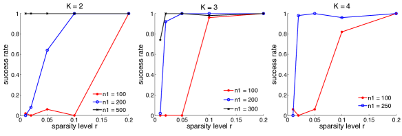
Figure 1: Results for Simulation 1: reporting the proportion of correct estimate of $K$ for stochastic block models, for $K=2,3,4$, under various sparsity levels $r\in\{0.01,0.02,0.05,0.1,0.2\}$, and various sizes of the first community $n_{1}$. The number of nodes is $1000$.

Simulation 2: general block structures and comparison to recursive bipartition. This simulation is designed to further investigate the proposed NCV method under general block structures of networks, and meanwhile to compare the proposed NCV method with the recursive testing procedure proposed in Bickel & Sarkar (2013). We generate symmetric $B$ randomly as follows. For each upper-triangle entry of $B$, we generate a random number from ${\rm Unif}(0,0.5)$. The upper bound $0.5$ is set to exclude unrealistically dense networks that are of less interest. We only use $B$ matrices whose $K$th singular values are in the upper three quarters and therefore have relatively well-formed $K$-block structures. The membership vector $g$ is generated from multinomial distribution $(n,\pi)$ with equal probability $\pi=(1/K,\dots,1/K)$. For each simulated data, we applied three-fold NCV method as well as the recursive bipartition algorithm developed in Bickel & Sarkar (2013) with $\alpha=0.01$. The basic idea of the recursive bipartition method is to divide the nodes into two clusters if $K=1$ is rejected at level $\alpha$, and then recursively test $K=1$ vs $K>1$ on each of the two sub-networks until failing to reject $K=1$. The success rates in 50 simulations for each combination of $n=600,1200$ and $K=1,2,3,4$ are shown in Figure 2. As expected, both methods benefit from a larger sample size (top row vs bottom row). The task of determining $K$ gets harder as the true number of communities gets larger (from left column to right column). The proposed NCV method performs uniformly better than the bipartition method. The NCV method is also much faster than the bipartition method, where the latter requires a small bootstrap sample to adjust the null distribution at each testing step. The simulation design suggests that the proposed NCV has very satisfactory performance under very general structures of $B$. For $n=1200$, the empirical success rate of NCV achieves 100% for $K=1,\ 2$, 84% for $K=3$, and 72% for $K=4$.

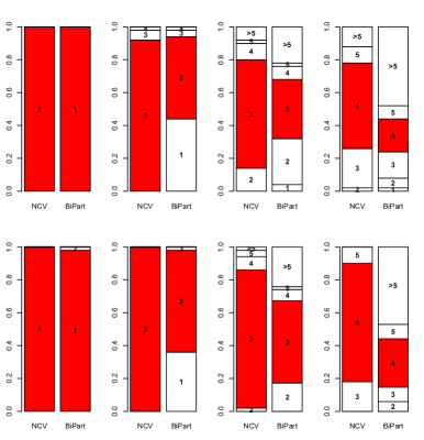
Figure 2: Results for Simulation 2: reporting the proportion of selected $K$ by NCV (the proposed method) and BiPart (Bickel & Sarkar (2013)), for true $K=1,2,3,4$ (from left to right), and sample size $n=600$ (top row) and $n=1200$ (bottom row).

Simulation 3: degree corrected block models. This simulation is designed to demonstrate the performance of selecting between the stochastic block model and the degree-corrected block model with simultaneous selection of $K$. We use a $B$ matrix whose diagonal is 0.25 and off-diagonal is 0.1, which gives a moderate sparsity level for stochastic block models. For degree-corrected block model, the degree parameter $\psi$ is generated from ${\rm Unif}(0.2,1)$, and normalized to have block-wise maximum value 1. The edges are generated according to 4. The network is much sparser in presence of the degree parameter $\psi$ and the inference problem is harder. Three-fold NCV is used to simultaneously choose the model type $T$ from $T=\text{``SBM''}$ or $T=\text{``DCBM''}$, and the number of communities $K$. Table 1 shows the proportion of correct model type selection $\hat{T}=T$ and proportion of correct choice of $K$ given correct model type selection. Data are generated 50 times from both the stochastic block model and the degree corrected block model, for each combination of $K=1,2,3,4$ and $n=300,600,1200$. We observe that when the true model type is stochastic block model, NCV can almost perfectly pick out the correct model and correct $K$ for various combinations of $K$ and $n$. As expected, a relatively larger sample size is needed to get good performance when the network is generated from a degree corrected block model. Our simulation shows that for $n=1200$, NCV can almost always pick out the correct DCBM model with the right $K$.

Table 1: Results for Simulation 3: proportion of selecting the correct model type, and choosing the correct $K$ given correct model type selection, from 50 independent simulations. The true models are generated from stochastic block models (SBM) or degree corrected block models (DCBM), for true $K=1,2,3,4$ and $n=300,600,1200$.

SBM DCBM $K=1$ $2$ $3$ $4$ $K=1$ $2$ $3$ $4$ $n=300$ $\hat{P}(\hat{T}=T)$ 1 1 1 1 1 0.68 0.44 0.42 $\hat{P}(\hat{K}=K|\hat{T}=T)$ 1 1 0.98 0.92 1 0.41 0 0 $n=600$ $\hat{P}(\hat{T}=T)$ 1 1 1 1 1 1 0.96 0.98 $\hat{P}(\hat{K}=K|\hat{T}=T)$ 1 1 1 0.98 1 1 0.42 0 $n=1200$ $\hat{P}(\hat{T}=T)$ 1 1 1 1 1 1 1 1 $\hat{P}(\hat{K}=K|\hat{T}=T)$ 1 1 1 0.98 1 1 1 1

Data example: political weblogs. The political blog data was collected and analyzed in Adamic & Glance (2005). The data set contains snapshots of over one thousand weblogs shortly before the 2004 U.S. Presidential Election, where the nodes are weblogs, and edges are hyperlinks. The nodes are labeled as being either liberal or conservative, which can be treated as two well-defined communities. The degree corrected block model is believed to fit better than the stochastic block model to this data with two communities (Karrer & Newman, 2011; Zhao et al., 2012; Jin, 2012). To illustrate the NCV method for simultaneously choosing between the regular stochastic block model and the degree corrected block model, and choosing the number of communities $K$, we apply three-fold NCV to the largest connected component in the network which contains 1222 nodes. The NCV method consistently selects the degree corrected block model with two communities. The cross-validated negative log-likelihood for all candidate models is plotted in Figure 3 for a typical block splitting. We repeated the NCV selection 100 times using independent random block splittings. The NCV method selected DCBM and $K=2$ in 99 out of 100 repetitions, where the one failure was due to non-convergence of $k$-means in spectral clustering.

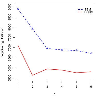
Figure 3: Results for the political blogs data: reporting the three-fold cross-validated negative log-likelihood of all candidate models from one random block splitting. Dashed line: stochastic block models; solid line: degree corrected block models. The results are consistent over 100 repeated random block splittings.

5 Discussion

Further extensions

In general, the network cross-validation approach proposed in this paper is applicable to network models where (i) edges form independently given an appropriate set of model parameters; and (ii) the edge probabilities can be estimated accurately using a subset of rows of the adjacency matrix. The stochastic block model and the degree corrected model are good examples satisfying these two properties. There are other popular network models in this category, such as the random dot-product graph. The random dot-product graph model (Young & Scheinerman, 2007) assumes that each node $i$ has an embedding $v_{i}$ on a subset of the $d$-dimensional unit sphere, and that given the embedding the edge between node $i$ and node $j$ is an independent Bernoulli random variable with parameter $\langle v_{i},v_{j}\rangle$. This is a special case of the latent space model (Hoff et al., 2002). The latent vectors can be accurately estimated using spectral methods (Sussman et al., 2013), which can be adapted naturally so that the model parameters can be estimated using only the fitting subset of node pairs in $A$.

Effect of the number of folds

In general, cross validation methods are insensitive to the number of folds. The same intuition empirically holds true for the proposed NCV method. However, there is slight difference between the NCV framework and the traditional cross-validation. Unlike traditional cross validation where each data point is included in a testing sample, In V-fold NCV only the diagonal blocks are used as testing samples and hence the proportion of edges included in testing samples is roughly $1/V$. On the other hand, the ratio between the sizes of fitting and testing samples in a single fold is $(V^{2}-1)$ to 1 for NCV, and $(V-1)$ to 1 for traditional cross-validation. Roughly speaking, having a larger value of $V$ will rapidly increase the estimation accuracy in the fitting stage but will reduce the testing sample size. In our numerical experiments we found $V=3$ a reasonable choice for most cases, which is roughly comparable to a 9-fold traditional cross validation in terms of the fitting and testing sample size ratio.

Appendix A Proofs

A.1 Proof of Theorem 2

Proof.

We focus on a single fold in NCV. The claimed results follow by summing over all folds. Again let $\mathcal{N}_{1}$ be the nodes corresponding to the fitting part and $\mathcal{N}_{2}$ be those in the testing part. Let $I_{l}=\{i\in\mathcal{N}_{2}:g_{i}=l,\}$ ($1\leq l\leq K$) and $\hat{I}_{k}=\{i\in\mathcal{N}_{2}:\hat{g}_{i}=k\}$ ($1\leq k\leq\tilde{K}$).

Case 1: $\tilde{K}<K$.

According to tail probability inequalities for hypergeometric distributions (see Lemma 5), with overwhelming probability over the random data splitting, the testing block $A^{(vv)}$ is also a realization of a $K$-block SBM satisfying assumptions A1–A2, with a different constant $\pi_{0}^{\prime}$.

When $\tilde{K}<K$, there exist $1\leq k\leq\tilde{K}$, $1\leq l_{1}<l_{2}\leq K$ such that $|\hat{I}_{k}\cap I_{l_{j}}|\geq|I_{l_{j}}|/\tilde{K}\geq\pi_{0}^{\prime}n/|\tilde{K}|$ for $j=1,2$. Because $B_{0}$ does not have identical rows, there exists $1\leq l_{3}\leq K$ such that $B_{0}(l_{1},l_{3})\neq B_{0}(l_{2},l_{3})$. There exists a $k^{\prime}$ such that $|\hat{I}_{k^{\prime}}\cap I_{l_{3}}|\geq|I_{l_{3}}|/\tilde{K}\geq\pi_{0}^{\prime}n/\tilde{K}$. We focus on the case $k\neq k^{\prime}$ and $l_{1},l_{2},l_{3}$ are distinct. The other cases, such as $k=k^{\prime}$ or $l_{1}=l_{3}$, or both, can be dealt with similarly. Without loss of generality, assume $k=1,k^{\prime}=2$, $l_{1}=1,l_{2}=2,l_{3}=3$.

Let $\mathcal{T}_{k,k^{\prime},l,l^{\prime}}$ be the set of unique pairs $(i,j)$ such that $i\in\hat{I}_{k}\cap I_{l}$, $j\in\hat{I}_{k^{\prime}}\cap I_{l}$, and $i\neq j$ (that is, $(i,j)$ and $(j,i)$ shall be counted as one unique pair in case of $k=k^{\prime}$ and $l=l^{\prime}$). Let $\hat{p}$ be the average of $A_{ij}$ over $(i,j)\in\mathcal{T}_{1,2,1,3}\cup\mathcal{T}_{1,2,2,3}$ and $\hat{p}_{k,k^{\prime},l,l^{\prime}}$ be the average of $A_{ij}$ over $(i,j)\in\mathcal{T}_{k,k^{\prime},l,l^{\prime}}$. Then, letting $L^{(v)}(A)$ be the terms in $L(A)$ corresponding to the $v$th fold,

$$\hat{L}^{(v)}(A,\tilde{K})-L^{(v)}(A)$$

$$= \sum_{k,k^{\prime},l,l^{\prime}}\sum_{(i,j)\in\mathcal{T}_{k,k^{\prime},l,l^{\prime}}}\left[(A_{ij}-\hat{P}_{ij})^{2}-(A_{ij}-P_{ij})^{2}\right]$$

$$= \sum_{k,k^{\prime},l,l^{\prime}}\sum_{(i,j)\in\mathcal{T}_{k,k^{\prime},l,l^{\prime}}}\left[(A_{ij}-\hat{B}_{k,k^{\prime}})^{2}-(A_{ij}-B_{l,l^{\prime}})^{2}\right]$$

$$= \sum_{(i,j)\in\mathcal{T}_{1,2,1,3}}\left[(A_{ij}-\hat{B}_{1,2})^{2}-(A_{ij}-B_{1,3})^{2}\right]+\sum_{(i,j)\in\mathcal{T}_{1,2,2,3}}\left[(A_{ij}-\hat{B}_{1,2})^{2}-(A_{ij}-B_{2,3})^{2}\right]$$

$$+\quad\sum_{(k,k^{\prime},l,l^{\prime})\notin\{(1,2,1,3),(1,2,2,3)\}}\sum_{(i,j)\in\mathcal{T}_{k,k^{\prime},l,l^{\prime}}}\left[(A_{ij}-\hat{B}_{k,k^{\prime}})^{2}-(A_{ij}-B_{l,l^{\prime}})^{2}\right]$$

$$\geq \sum_{(i,j)\in\mathcal{T}_{1,2,1,3}}\left[(A_{ij}-\hat{p})^{2}-(A_{ij}-B_{1,3})^{2}\right]+\sum_{(i,j)\in\mathcal{T}_{1,2,2,3}}\left[(A_{ij}-\hat{p})^{2}-(A_{ij}-B_{2,3})^{2}\right]$$

$$+\quad\sum_{(k,k^{\prime},l,l^{\prime})\notin\{(1,2,1,3),(1,2,2,3)\}}\sum_{(i,j)\in\mathcal{T}_{k,k^{\prime},l,l^{\prime}}}\left[(A_{ij}-\hat{p}_{k,k^{\prime},l,l^{\prime}})^{2}-(A_{ij}-B_{l,l^{\prime}})^{2}\right]$$

$$= I+II+III.$$

Let $\lambda=|\mathcal{T}_{1,2,1,3}|/(|\mathcal{T}_{1,2,1,3}+\mathcal{T}_{1,2,2,3}|)$. Then $\pi_{0}^{\prime 2}/(\tilde{K}^{2}+\pi_{0}^{\prime 2})\leq\lambda\leq\tilde{K}^{2}/(\tilde{K}^{2}+\pi_{0}^{\prime 2})$, and $\hat{p}=\lambda\hat{p}_{1,2,1,3}+(1-\lambda)\hat{p}_{1,2,2,3}$. If $|\mathcal{T}_{k,k^{\prime},l,l^{\prime}}|>0$, using Bernstein’s inequality we have

$$|\hat{p}_{k,k^{\prime},l,l^{\prime}}-B_{l,l^{\prime}}|=O_{P}\left(\sqrt{\frac{\rho_{n}}{|\mathcal{T}_{k,k^{\prime},l,l^{\prime}}|}}\right)\,.$$ (7)

$$I= |\mathcal{T}_{1,2,1,3}|\left[(\hat{p}-\hat{p}_{1,2,1,3})^{2}-(\hat{p}_{1,2,1,3}-B_{1,3})^{2}\right]$$

$$= |\mathcal{T}_{1,2,1,3}|\left[(1-\lambda)^{2}(\hat{p}_{1,2,1,3}-\hat{p}_{1,2,2,3})^{2}-(\hat{p}_{1,2,1,3}-B_{1,3})^{2}\right]$$

$$\geq |\mathcal{T}_{1,2,1,3}|\bigg{[}\frac{(1-\lambda)^{2}}{2}(B_{1,3}-B_{2,3})^{2}-(1-\lambda)^{2}\left((\hat{p}_{1,2,1,3}-B_{1,3})-(\hat{p}_{1,2,2,3}-B_{2,3})\right)^{2}$$

$$\qquad\qquad-(\hat{p}_{1,2,1,3}-B_{1,3})^{2}\bigg{]}$$

$$\geq |\mathcal{T}_{1,2,1,3}|\bigg{[}\frac{(1-\lambda)^{2}}{2}(B_{1,3}-B_{2,3})^{2}-2(1-\lambda)^{2}\left(\hat{p}_{1,2,1,3}-B_{1,3}\right)^{2}$$

$$\qquad\qquad-2(1-\lambda)^{2}\left(\hat{p}_{1,2,2,3}-B_{2,3}\right)^{2}-(\hat{p}_{1,2,1,3}-B_{1,3})^{2}\bigg{]}$$

$$\geq c(n\rho_{n})^{2}+O_{P}(\rho_{n})\,.$$

where the constant $c$ depending on $\pi_{0}$, $B_{0}$ and $\tilde{K}$ only, the first term in the last inequality comes from the fact that $|\mathcal{T}_{1,2,1,3}|\geq\pi_{0}^{2}n^{2}/\tilde{K}^{2}$ and $|B_{1,2}-B_{1,3}|\geq c^{\prime}\rho_{n}$ for some $c^{\prime}$ depending only on $B_{0}$, the second term comes from (7) and the fact that $|T_{1,2,1,3}|\asymp|T_{1,2,2,3}|$.

Similarly,

$$II\geq c(n\rho_{n})^{2}+O_{P}(\rho_{n})\,.$$

and

$$III\geq-\sum_{(k,k^{\prime},l,l^{\prime})\notin\{(1,2,1,3),(1,2,2,3)\}}|\mathcal{T}_{k,k^{\prime},l,l^{\prime}}|(\hat{p}_{k,k^{\prime},l,l^{\prime}}-B_{l,l^{\prime}})^{2}=O_{P}(\rho_{n})\,.$$

Case 2: $\tilde{K}=K$ with exactly consistent recovery
In this case we focus on the event $\hat{g}=g$, which has $1-o(1)$ probability. Then $\epsilon_{n}\coloneqq\sup_{1\leq l,l^{\prime}\leq K}|\hat{B}_{l,l^{\prime}}-B_{l,l^{\prime}}|=O_{P}(\sqrt{\rho_{n}}/n)$ by Bernstein’s inequality and $\hat{B}_{l,l^{\prime}}$ are independent with $A_{ij}$ for $(i,j)$ in the testing set.

For $1\leq k,k^{\prime}\leq K$, let $\mathcal{T}_{l,l^{\prime}}$ be the collection of pairs $(i,j)$ in the testing set such that $i\in I_{k}$, $j\in I_{k^{\prime}}$ and $i\neq j$.

$$\left|\hat{L}^{(v)}(A,\tilde{K})-L^{(v)}(A)\right|\leq \sum_{k,k^{\prime}}\sum_{(i,j)\in\mathcal{T}_{k,k^{\prime}}}\left|(A_{ij}-\hat{B}_{k,k^{\prime}})^{2}-(A_{ij}-B_{k,k^{\prime}})^{2}\right|$$

$$= \sum_{k,k^{\prime}}\sum_{(i,j)\in\mathcal{T}_{k,k^{\prime}}}\left|-2A_{ij}(\hat{B}_{k,k^{\prime}}-B_{k,k^{\prime}})+(\hat{B}_{k,k^{\prime}}+B_{k,k^{\prime}})(\hat{B}_{k,k^{\prime}}-B_{k,k^{\prime}})\right|$$

$$\leq \sum_{k,k^{\prime}}\sum_{(i,j)\in\mathcal{T}_{k,k^{\prime}}}\left[2\epsilon_{n}A_{ij}+(2\rho_{n}+\epsilon_{n})\epsilon_{n}\right]$$

$$\leq O_{p}(n^{2}\rho_{n})\epsilon_{n}+n^{2}(2\rho_{n}+\epsilon_{n})\epsilon_{n}=O_{P}(n\rho_{n}^{3/2})\,.$$

Because $n\rho_{n}^{3/2}=o((n\rho_{n})^{2})$, we have

$$P(\hat{K}<K)\leq \sum_{\tilde{K}<K}P\left[\hat{L}(A,\tilde{K})<\hat{L}(A,K)\right]$$

$$\leq \sum_{\tilde{K}<K}\sum_{1\leq v\leq V}P\left[\hat{L}^{(v)}(A,\tilde{K})<\hat{L}^{(v)}(A,K)\right]=o(1)\,.$$

This proves part (a) of Corollary 3.

Case 3: $\tilde{K}=K$ with approximately consistent recovery

Without loss of generality we assume the optimal permutation to match $\hat{g}$ and $g$ is the identity. Let $\hat{\mathcal{U}}_{k,k^{\prime}}$ be the set of distinct pairs $(i,j)$ in the fitting subset such that $\hat{g}_{i}=k$, $\hat{g}_{i}=k^{\prime}$, and $i\neq j$. Let $\mathcal{U}_{k,k^{\prime}}$ be the set of distinct pairs $(i,j)$ in the fitting subset such that $g_{i}=k$, $g_{i}=k^{\prime}$, and $i\neq j$. Let $S=\bigcup_{k=1}^{K}\hat{I}_{k}\Delta I_{k}$, $\mathcal{S}=\bigcup_{k,k^{\prime}}\hat{\mathcal{U}}_{k,k^{\prime}}\Delta\mathcal{U}_{k,k^{\prime}}$. On the event $|S|\leq\eta_{n}n$, under Assumptions (A1) and (A2) we have $|\mathcal{S}|=O(\eta_{n}n^{2})$, and hence $|\hat{\mathcal{U}}_{k,k^{\prime}}|=|\mathcal{U}_{k,k^{\prime}}|(1+O(\eta_{n}))$ for all $k,k^{\prime}$.

$$\left|\hat{B}_{k,k^{\prime}}-B_{k,k^{\prime}}\right|$$

$$= \left|\frac{1}{|\hat{\mathcal{U}}_{k}|}\left(\sum_{(i,j)\in\mathcal{U}_{k,k^{\prime}}}A_{ij}\right)-B_{k,k^{\prime}}\right|+\frac{1}{|\hat{\mathcal{U}}_{k,k^{\prime}}|}\sum_{(i,j)\in\hat{\mathcal{U}}_{k,k^{\prime}}\Delta\mathcal{U}_{k,k^{\prime}}}A_{ij}$$

$$\leq \frac{|\mathcal{U}_{k,k^{\prime}}|}{|\hat{\mathcal{U}}_{k,k^{\prime}}|}\left|\frac{1}{|\mathcal{U}_{k,k^{\prime}}|}\sum_{(i,j)\in\mathcal{U}_{k,k^{\prime}}}A_{ij}-B_{k,k^{\prime}}\right|+\left|\frac{|\mathcal{U}_{k,k^{\prime}}|}{|\hat{\mathcal{U}}_{k,k^{\prime}}|}-1\right|B_{k,k^{\prime}}+\frac{1}{|\hat{\mathcal{U}}_{k,k^{\prime}}|}\sum_{(i,j)\in\hat{\mathcal{U}}_{k,k^{\prime}}\Delta\mathcal{U}_{k,k^{\prime}}}A_{ij}$$

$$\leq (1+O(\eta_{n}))O_{P}\left(\sqrt{B_{k,k^{\prime}}/|\mathcal{U}_{k,k^{\prime}}|}\right)+O(\eta_{n})B_{k,k^{\prime}}+(1+O(\eta_{n}))\eta_{n}$$

$$= O_{P}(\rho_{n}^{1/2}n^{-1}+\eta_{n})\,.$$

Focusing on the $v$th fold in cross-validation, we similarly have, letting $\epsilon_{n}=\sup_{k,k^{\prime}}|\hat{B}_{k,k^{\prime}}-B_{k,k^{\prime}}|$,

$$\left|\hat{L}^{(v)}(A,\tilde{K})-L^{(v)}(A)\right|\leq O_{p}(n^{2}(\rho_{n}+\epsilon_{n})\epsilon_{n})=O_{p}(n\rho_{n}^{3/2}+n^{2}\rho_{n}\eta_{n})\,.\qed$$

A.2 Proof of Theorem 1 and Theorem 4

Next we prove Theorem 1 and Theorem 4. Let $P$ be the $n\times n$ matrix such that $P_{ij}=B_{g_{i}g_{j}}$. For a particular fold split in NCV, let $A^{(1)}$ and $P^{(1)}$ be the testing rectangular submatrix of $A$ and $P$ respectively. Let $\mathcal{N}_{j,k}^{*}$ be the nodes in subsample $\mathcal{N}_{j}$ belonging to community $k$ and $n_{j,k}^{*}=|\mathcal{N}_{j,k}^{*}|$ ($j=1,2$, $k=1,...,K$). For any matrix $M$, let $\sigma_{K}(M)$ be its $K$th largest singular value. In the statement of results and the proof, constants $c$, $C$ may take different values from line to line. We let $\|M\|=\sigma_{1}(M)$ be the spectral norm of $M$ and $\|M\|_{F}=(\sigma_{1}^{2}(M)+\sigma_{2}^{2}(M)+...)^{1/2}$ be the Frobenious norm.

A.2.1 Preliminary results

The following technical lemmas are needed in the proof of Theorem 1 and Theorem 4.

Lemma 5 (Size of split community).

Under Assumption (A1), for $n$ large enough we have $\min_{k}n_{1,k}^{*}\geq\pi_{0}n/(2V)$, with probability at least $1-n^{-1}/2$.

The proof of this lemma follows from a simple application of large deviation bounds for hypergeometric random variables (Skala, 2013) combined with union bound and is omitted.

Lemma 6 (Spectral norm error of partial adjacency matrix).

Let $A$ be the adjacency matrix generated from a degree corrected block model satisfying Assumption A2, with $\rho_{n}\geq c\log n/n$ for a positive constant $c$. Let $\tilde{A}$ be an arbitrary subset of rows of $A$ and $\tilde{P}$ be the corresponding submatrix of $P$. We have, for some constant $C$,

$$P\left(\|\tilde{A}-\tilde{P}\|\leq C\sqrt{n\rho_{n}}\right)\geq 1-n^{-1}/2\,.$$

Proof.

Observe that $\|\tilde{A}-\tilde{P}\|\leq\|A-P\|$. The claimed result follows easily from Theorem 5.2 of Lei & Rinaldo (2013), where it has been shown that with high probability $\|A-P\|\leq C\sqrt{n\rho_{n}}$. ∎

Lemma 6 covers both regular SBM and DCBM. It implies that $\|A^{(1)}-P^{(1)}\|\leq C\sqrt{n\rho_{n}}$ with high probability.

Lemma 7 (Singular subspace error bound).

Let $\hat{M}$, $M$ be two matrices of same dimension, and $\hat{U}$ and $U$ be $n\times K$ orthonormal matrices corresponding to the top $K$ right singular vectors of $\hat{M}$ and $M$, respectively. Then there exists a $K\times K$ orthogonal matrix $Q$ such that

$$\|\hat{U}-UQ\|\leq\frac{2\sqrt{2}\|\hat{M}-M\|}{\sigma_{K}(M)}\,.$$

Proof.

If $\|\hat{M}-M\|\leq\sigma_{K}(M)/2$, then using Wedin $\sin\Theta$ theorem (Wedin, 1972) and Weyl’s inequality there exists an orthogonal $Q$ such that $\|\hat{U}-UQ\|\leq\|\hat{M}-M\|/(\sigma_{K}(M)-\|\hat{M}-M\|)\leq 2\|\hat{M}-M\|/\sigma_{K}(M)$. If $\|\hat{M}-M\|\geq\sigma_{K}(M)/2$, then $\|\hat{U}-UQ\|\leq 1\leq 2\|\hat{M}-M\|/\sigma_{K}(M)$. ∎

Remark. The orthogonal matrix $Q$ will have no particular impact on the argument below. For presentation simplicity, we assume, without loss of generality, that $Q=I$ in the rest of the proof.

Lemma 8 (Lemma 5.3 of Lei & Rinaldo (2013)).

Let $\hat{U}$ and $U$ be two $n\times K$ matrices such that $U$ contains $K$ distinct rows. Let $\delta$ be the minimum distance between two distinct rows of $U$, and $g$ be the membership vector given by clustering the rows of $U$. Let $\hat{g}$ be the output of a $k$-means clustering algorithm on $\hat{U}$, with objective value no larger than a constant factor of the global optimum. Assume that $\|\hat{U}-U\|_{F}\leq cn\delta$ for some small enough constant $c$. Then $\hat{g}$ agrees with $g$ on all but $c^{-1}\|\hat{U}-U\|_{F}\delta^{-1}$ nodes after an appropriate label permutation.

For the proof of Theorem 4, we need the analogous version of Lemma 8 for the k-median algorithm, which is a simple adaptation of Lemma 8. For a matrix $M$, $\|M\|_{2,1}$ denotes the sum of $\ell_{2}$ norms of the rows in $M$.

Lemma 9.

Let $\hat{U}$ and $U$ be two $n\times K$ matrices such that $U$ contains $K$ distinct rows. Let $\delta$ be the minimum distance between two distinct rows of $U$, and $g$ be the membership vector given by clustering the rows of $U$. Let $\hat{g}$ be the output of a $k$-median clustering algorithm on $\hat{U}$, with objective value no larger than a constant factor of the global optimum. Assume that $\|\hat{U}-U\|_{2,1}\leq cn\delta$ for some small enough constant $c$ and that $g$ satisfies Assumption A2. Then $\hat{g}$ agrees with $g$ on all but $c^{-1}\|\hat{U}-U\|_{2,1}\delta^{-1}$ nodes after an appropriate label permutation.

A.2.2 Proof of Theorem 1

Proof of Theorem 1.

Let $G$ be the $n\times K$ matrix with $G_{ij}=1$ if $j=g_{i}$, and $G_{ij}=0$ otherwise. Let $G^{(1)}$ be the submatrix of $G$ containing rows in $\mathcal{N}_{1}$. Then $P^{(1)}=G^{(1)}BG^{T}=G\tilde{B}\tilde{G}^{T}$, where $\tilde{G}$ is an $n\times K$ matrix obtained by normalizing the columns of $G$. and $\tilde{B}$ is a $K\times K$ matrix after corresponding column scaling of $B$. It is easy to check that $\tilde{G}$ has orthonormal columns and hence the top $K$-dimensional right singular subspace of $P^{(1)}$ is spanned by $U=\tilde{G}Q$, for any $K\times K$ orthogonal matrix $Q$. Thus $U$ contains $K$ distinct rows and the distance between two distinct rows is of order at least $1/\sqrt{n}$.

We focus on the event that $\min_{k}n_{1,k}^{*}\geq\pi_{0}n/(2V)$ and $\|A^{(1)}-P^{(1)}\|\leq C\sqrt{n\alpha_{n}}$, which has probability at least $1-n^{-1}$ according to Lemmas 5 and 6. Then it can be directly verified that $\sigma_{K}(P^{(1)})\geq Cn\alpha_{n}$ because the $K$th largest singular values of both $G^{(1)}$ and $G$ are of order at least $\sqrt{n}$. Then Lemma 7 implies that $\hat{U}$ and $U$, the matrices consisting of $n\times K$ top singular vectors of $A^{(1)}$ and $P^{(1)}$, satisfy, with appropriate choice of $Q$,

$$\|\hat{U}-U\|_{F}^{2}\leq C\frac{1}{n\alpha_{n}}\,.$$

Then applying Lemma 8, we know that the $k$-means clustering algorithm misclusters no more than $C/\alpha_{n}$ nodes. ∎

A.2.3 Proof of Theorem 4

Proof of Theorem 4.

Let $\Psi$ be an $n\times K$ matrix such that $\Psi_{ij}=\psi^{\prime}_{i}$ if $j=g_{i}$ and $\Psi_{ij}=0$ otherwise. Let $\Psi^{(1)}$ be the corresponding submatrix of $\Psi$ with rows in $\mathcal{N}_{1}$. Then $P^{(1)}=\Psi^{(1)}\tilde{B}\Psi$, where $\tilde{B}$ is a $K\times K$ matrix obtained after corresponding row/column scaling of $B$. It is easy to check that $\Psi$ is orthonormal so that the top $K$-dimensional right singular subspace of $P^{(1)}$ is spanned by $U=\Psi Q$ for any $K\times K$ orthogonal $Q$. It follows that the norm of $i$th row of $U$ is $\psi^{\prime}_{i}$, and that any two rows of $U$ in distinct communities are orthogonal. Let $\tilde{U}$ and $\tilde{U}^{*}$ be the row-normalized versions of $\hat{U}$ and $U$, respectively. Then $\tilde{U}^{*}$ contains $K$ distinct rows and the distance between any two distinct rows of $\tilde{U}^{*}$ is $\sqrt{2}$.

We will focus on the event that $\min_{k}n_{1,k}^{*}\geq c_{0}\pi_{0}n/2$ and $\|A^{(1)}-P^{(1)}\|\leq C\sqrt{n\alpha_{n}}$, which has probability at least $1-n^{-1}$ according to Lemmas 5 and 6. Applying Lemma 7 we have,

$$\|\hat{U}-U\|_{F}^{2}\leq C/(n\alpha_{n})\,,$$

where we take the matrix $Q$ in Lemma 7 as identity. Because the minimum row norm of $U$ is at least $\psi_{0}/\sqrt{n}$, the number of zero rows in $\hat{U}$ is at most $\|\hat{U}-U\|_{F}^{2}/(\psi_{0}/\sqrt{n})^{2}=O(\alpha_{n}^{-1})=o(\sqrt{n/\alpha_{n}})$. In the rest of the proof we can safely assume that $\hat{U}$ has no zero rows.

Now let $u_{i}$, $\hat{u}_{i}$ be the $i$th row of $U$, $\hat{U}$, respectively. We have, using the fact that $\left\|(u/\|u\|-v/\|v\|)\right\|\leq 2\|u-v\|/\|v\|$ for all vectors $u,v$ of same dimension, Cauchy-Schwartz, and Assumption A3,

$$\|\tilde{U}-\tilde{U}^{*}\|_{2,1}\leq 2\sum_{i=1}^{n}\frac{\|\hat{u}_{i}-u_{i}\|}{\|u_{i}\|}=2\sum_{i=1}^{n}\frac{\|\hat{u}_{i}-u_{i}\|}{\psi_{i}^{\prime}}$$

$$\leq 2\|\hat{U}-U\|_{F}\left(\sum_{i=1}^{n}(\psi_{i}^{\prime})^{-2}\right)^{1/2}\leq 2\psi_{0}^{-1}n\|\hat{U}-U\|_{F}\leq C\sqrt{n/\alpha_{n}}\,.$$

Applying Lemma 9 to $\tilde{U}$ and $\tilde{U}^{*}$, we conclude that $\hat{g}$ agrees with $g$ on all but $O(\sqrt{n/\alpha_{n}})$ nodes.

Recall that $\|u_{i}\|=\psi_{i}^{\prime}$ for all $i$. Then Cauchy-Schwartz implies that

$$\|\hat{\psi}^{\prime}-\psi^{\prime}\|_{1}\leq \sum_{i=1}^{n}\|\hat{u}_{i}-u_{i}\|\leq\sqrt{n}\|\hat{U}-U\|_{F}\leq C\alpha_{n}^{-1/2}\,.$$ (8)

By Assumptions (A2) and (A3) we have $\inf_{i}\psi_{i}^{\prime}\geq Cn^{-1/2}$ for some constant $C$.

Let $S_{n}=\{i:|\hat{\psi}_{i}^{\prime}-\psi_{i}^{\prime}|\leq n^{-1/2}(n^{1/3}\alpha_{n})^{-1/2}\}$. Then for all $i\in S_{n}$, we have $\hat{\psi}_{i}^{\prime}=\psi_{i}^{\prime}(1+o(1))$ and

$$|S_{n}^{c}|\leq\frac{\|\hat{\psi}^{\prime}-\psi^{\prime}\|_{1}}{n^{-2/3}\alpha_{n}^{-1/2}}\leq Cn^{2/3}\,.$$ (9)

For $1\leq k<k^{\prime}\leq K$, consider the oracle estimator

$$\hat{B}_{k,k^{\prime}}^{\prime*}=\frac{\sum_{i\in\mathcal{N}_{1,k}^{*},j\in\mathcal{N}_{1,k^{\prime}}^{*}\cup\mathcal{N}_{2,k^{\prime}}^{*}}A_{ij}}{\sum_{i\in\mathcal{N}_{1,k}^{*},j\in\mathcal{N}_{1,k^{\prime}}^{*}\cup\mathcal{N}_{2,k^{\prime}}^{*}}\psi^{\prime}_{i}\psi^{\prime}_{j}}\,.$$

It is obvious that $\hat{P}^{*}_{ij}=\psi_{i}^{\prime}\psi_{j}^{\prime}\hat{B}_{g_{i}g_{j}}^{\prime*}=(1+o_{P}(1))\psi_{i}\psi_{j}B_{g_{i}g_{j}}=(1+o_{P}(1))P_{ij}$. As a result, the claim in part (b) of the theorem follows if we can show that $\hat{B}_{k,k^{\prime}}^{\prime}=(1+o_{P}(1))\hat{B}_{k,k^{\prime}}^{\prime*}$ because for all but a vanishing proportion of pairs $(i,j)$ we have $(\hat{g}_{i},\hat{g}_{j})=(g_{i},g_{j})$ and $\hat{\psi}_{i}^{\prime}\hat{\psi}_{j}^{\prime}=\psi_{i}^{\prime}\psi_{j}^{\prime}(1+o(1))$ in view of (9). To this end, we compare

$$n^{-1}\hat{B}_{k,k^{\prime}}^{\prime}=\frac{\sum_{i\in\mathcal{N}_{1,k},j\in\mathcal{N}_{1,k^{\prime}}\cup\mathcal{N}_{2,k^{\prime}}^{*}}A_{ij}}{\sum_{i\in\mathcal{N}_{1,k},j\in\mathcal{N}_{1,k^{\prime}}\cup\mathcal{N}_{2,k^{\prime}}}(\sqrt{n}\hat{\psi}^{\prime}_{i})(\sqrt{n}\hat{\psi}^{\prime}_{j})}$$

with

$$n^{-1}\hat{B}_{k,k^{\prime}}^{\prime*}=\frac{\sum_{i\in\mathcal{N}_{1,k}^{*},j\in\mathcal{N}_{1,k^{\prime}}^{*}\cup\mathcal{N}_{2,k^{\prime}}^{*}}A_{ij}}{\sum_{i\in\mathcal{N}_{1,k}^{*},j\in\mathcal{N}_{1,k^{\prime}}^{*}\cup\mathcal{N}_{2,k^{\prime}}^{*}}(\sqrt{n}\psi^{\prime}_{i})(\sqrt{n}\psi^{\prime}_{j})}\,.$$

Note that $\sqrt{n}\psi_{i}^{\prime}\asymp 1$ for all $i$. It is easy to check that the numerators differ by at most $o(n^{5/3})$. For the denominators, first we compare the denominator of $n^{-1}\hat{B}_{k,k^{\prime}}^{\prime*}$ with

$$\sum_{i\in\mathcal{N}_{1,k},j\in\mathcal{N}_{1,k^{\prime}}\cup\mathcal{N}_{2,k^{\prime}}}(\sqrt{n}\psi^{\prime}_{i})(\sqrt{n}\psi^{\prime}_{j})\,.$$ (10)

It straightforward to check that their ratio tends to 1, because the index sets of these two summations differ by a vanishing proportion. Now compare (10) with the denominator of $n^{-1}\hat{B}_{k,k^{\prime}}^{\prime}$. We have

$$\sum_{i\in\mathcal{N}_{1,k},j\in\mathcal{N}_{1,k^{\prime}}\cup\mathcal{N}_{2,k^{\prime}}}(\sqrt{n}\hat{\psi}^{\prime}_{i})(\sqrt{n}\hat{\psi}^{\prime}_{j})= \left(\sum_{i\in\mathcal{N}_{1,k}}\sqrt{n}\hat{\psi}_{i}^{\prime}\right)\left(\sum_{j\in\mathcal{N}_{1,k^{\prime}}\cup\mathcal{N}_{2,k^{\prime}}}\sqrt{n}\hat{\psi}_{j}^{\prime}\right)$$

$$= (1+o(1))\left(\sum_{i\in\mathcal{N}_{1,k}}\sqrt{n}\psi_{i}^{\prime}\right)\left(\sum_{j\in\mathcal{N}_{1,k^{\prime}}\cup\mathcal{N}_{2,k^{\prime}}}\sqrt{n}\psi_{j}^{\prime}\right)$$

$$= (1+o(1))\sum_{i\in\mathcal{N}_{1,k},j\in\mathcal{N}_{1,k^{\prime}}\cup\mathcal{N}_{2,k^{\prime}}}(\sqrt{n}\psi^{\prime}_{i})(\sqrt{n}\psi^{\prime}_{j})\,,$$

where the second line follows from the fact $\sum_{i\in\mathcal{N}_{j,k}}\hat{\psi}_{i}^{\prime}=(1+o(1))\sum_{i\in\mathcal{N}_{j,k}}\psi_{i}^{\prime}$ for all $j\in\{1,2\}$, $1\leq k\leq K$, which is a consequence of (8). Now we conclude that the denominators of $n^{-1}\hat{B}_{k,k^{\prime}}^{\prime}$ and $n^{-1}\hat{B}_{k,k^{\prime}}^{\prime*}$ are both of order at least $n^{2}$ with ratio tending to one. Therefore, the absolute difference between $n^{-1}\hat{B}_{k,k^{\prime}}^{\prime}$ and $n^{-1}\hat{B}_{k,k^{\prime}}^{\prime*}$ is $o(n^{-1/3})$ which is $o(n^{-1}\hat{B}_{k,k^{\prime}}^{\prime*})$. The same argument can be used for the case $k=k^{\prime}$. ∎

References

- Abbe et al. (2014) Abbe, E., Bandeira, A. S., & Hall, G. (2014). Exact recovery in the stochastic block model. arXiv preprint arXiv:1405.3267.
- Adamic & Glance (2005) Adamic, L. A., & Glance, N. (2005). The political blogosphere and the 2004 us election: divided they blog. In Proceedings of the 3rd international workshop on Link discovery, (pp. 36–43). ACM.
- Airoldi et al. (2008) Airoldi, E. M., Blei, D. M., Fienberg, S. E., & Xing, E. P. (2008). Mixed membership stochastic blockmodels. The Journal of Machine Learning Research, 9, 1981–2014.
- Anandkumar et al. (2014) Anandkumar, A., Ge, R., Hsu, D., & Kakade, S. M. (2014). A tensor approach to learning mixed membership community models. Journal of Machine Learning Research, 15, 2239–2312.
- Bickel & Chen (2009) Bickel, P. J., & Chen, A. (2009). A nonparametric view of network models and newman–girvan and other modularities. Proceedings of the National Academy of Sciences, 106(50), 21068–21073.
- Bickel & Sarkar (2013) Bickel, P. J., & Sarkar, P. (2013). Hypothesis testing for automated community detection in networks. arXiv preprint arXiv:1311.2694.
- Charikar et al. (1999) Charikar, M., Guha, S., Tardos, É., & Shmoys, D. B. (1999). A constant-factor approximation algorithm for the k-median problem. In Proceedings of the thirty-first annual ACM symposium on Theory of computing, (pp. 1–10). ACM.
- Chaudhuri et al. (2012) Chaudhuri, K., Chung, F., & Tsiatas, A. (2012). Spectral clustering of graphs with general degrees in the extended planted partition model. JMLR: Workshop and Conference Proceedings, 2012, 35.1–35.23.
- Chen et al. (2012) Chen, Y., Sanghavi, S., & Xu, H. (2012). Clustering sparse graphs. In P. Bartlett, F. Pereira, C. Burges, L. Bottou, & K. Weinberger (Eds.) Advances in Neural Information Processing Systems 25, (pp. 2213–2221).
- Decelle et al. (2011) Decelle, A., Krzakala, F., Moore, C., & Zdeborová, L. (2011). Asymptotic analysis of the stochastic block model for modular networks and its algorithmic applications. Physical Review E, 84(6), 066106.
- Faust & Wasserman (1992) Faust, K., & Wasserman, S. (1992). Blockmodels: Interpretation and evaluation. Social networks, 14(1), 5–61.
- Fishkind et al. (2013) Fishkind, D. E., Sussman, D. L., Tang, M., Vogelstein, J. T., & Priebe, C. E. (2013). Consistent adjacency-spectral partitioning for the stochastic block model when the model parameters are unknown. SIAM Journal on Matrix Analysis and Applications, 34(1), 23–39.
- Hoff (2008) Hoff, P. (2008). Modeling homophily and stochastic equivalence in symmetric relational data. In Advances in Neural Information Processing Systems, (pp. 657–664).
- Hoff et al. (2002) Hoff, P. D., Raftery, A. E., & Handcock, M. S. (2002). Latent space approaches to social network analysis. Journal of the american Statistical association, 97(460), 1090–1098.
- Holland et al. (1983) Holland, P. W., Laskey, K. B., & Leinhardt, S. (1983). Stochastic blockmodels: First steps. Social networks, 5(2), 109–137.
- Jin (2012) Jin, J. (2012). Fast community detection by SCORE. arXiv:1211.5803.
- Karrer & Newman (2011) Karrer, B., & Newman, M. E. (2011). Stochastic blockmodels and community structure in networks. Physical Review E, 83(1), 016107.
- Kemp et al. (2006) Kemp, C., Tenenbaum, J. B., Griffiths, T. L., Yamada, T., & Ueda, N. (2006). Learning systems of concepts with an infinite relational model. In AAAI, vol. 3, (p. 5).
- Krzakala et al. (2013) Krzakala, F., Moore, C., Mossel, E., Neeman, J., Sly, A., Zdeborová, L., & Zhang, P. (2013). Spectral redemption in clustering sparse networks. Proceedings of the National Academy of Sciences, 110(52), 20935–20940.
- Latouche et al. (2012) Latouche, P., Birmele, E., & Ambroise, C. (2012). Variational bayesian inference and complexity control for stochastic block models. Statistical Modelling, 12(1), 93–115.
- Lei (2014) Lei, J. (2014). A goodness-of-fit test for stochastic block models. arXiv preprint arXiv:1412.4857.
- Lei & Rinaldo (2013) Lei, J., & Rinaldo, A. (2013). Consistency of spectral clustering in sparse stochastic block models. arXiv preprint arXiv:1312.2050.
- Lei & Zhu (2014) Lei, J., & Zhu, L. (2014). A generic sample splitting approach for refined community recovery in stochastic block models. arXiv preprint arXiv:1411.1469.
- Li & Svensson (2013) Li, S., & Svensson, O. (2013). Approximating k-median via pseudo-approximation. In Proceedings of the 45th annual ACM symposium on Symposium on theory of computing, (pp. 901–910). ACM.
- Massoulie (2013) Massoulie, L. (2013). Community detection thresholds and the weak ramanujan property. arXiv preprint arXiv:1311.3085.
- McDaid et al. (2013) McDaid, A. F., Murphy, T. B., Friel, N., & Hurley, N. J. (2013). Improved bayesian inference for the stochastic block model with application to large networks. Computational Statistics & Data Analysis, 60, 12–31.
- McSherry (2001) McSherry, F. (2001). Spectral partitioning of random graphs. In Foundations of Computer Science, 2001. Proceedings. 42nd IEEE Symposium on, (pp. 529–537). IEEE.
- Mossel et al. (2013) Mossel, E., Neeman, J., & Sly, A. (2013). A proof of the block model threshold conjecture. arXiv preprint arXiv:1311.4115.
- Neville et al. (2012) Neville, J., Gallagher, B., Eliassi-Rad, T., & Wang, T. (2012). Correcting evaluation bias of relational classifiers with network cross validation. Knowledge and information systems, 30(1), 31–55.
- Newman (2006) Newman, M. E. (2006). Modularity and community structure in networks. Proceedings of the National Academy of Sciences, 103(23), 8577–8582.
- Newman & Girvan (2004) Newman, M. E., & Girvan, M. (2004). Finding and evaluating community structure in networks. Physical review E, 69(2), 026113.
- Saldana et al. (2014) Saldana, D. F., Yu, Y., & Feng, Y. (2014). How many communities are there? arXiv preprint arXiv:1412.1684.
- Skala (2013) Skala, M. (2013). Hypergeometric tail inequalities: ending the insanity. arXiv preprint arXiv:1311.5939.
- Sussman et al. (2013) Sussman, D. L., Tang, M., & Priebe, C. E. (2013). Universally consistent latent position estimation and vertex classification for random dot product graphs. Pattern Analysis and Machine Intelligence, IEEE Transactions on, 36(1), 48–57.
- Vu (2014) Vu, V. (2014). A simple svd algorithm for finding hidden partitions. arXiv preprint arXiv:1404.3918.
- Wang & Bickel (2015) Wang, Y., & Bickel, P. J. (2015). Likelihood-based model selection for stochastic block models. arXiv preprint arXiv:1502.02069.
- Wedin (1972) Wedin, P.-Å. (1972). Perturbation bounds in connection with singular value decomposition. BIT Numerical Mathematics, 12(1), 99–111.
- Yan et al. (2014) Yan, X., Shalizi, C., Jensen, J. E., Krzakala, F., Moore, C., Zdeborová, L., Zhang, P., & Zhu, Y. (2014). Model selection for degree-corrected block models. Journal of Statistical Mechanics: Theory and Experiment, 2014(5), P05007.
- Young & Scheinerman (2007) Young, S. J., & Scheinerman, E. R. (2007). Random dot product graph models for social networks. In Algorithms and models for the web-graph, (pp. 138–149). Springer.
- Zhao et al. (2011) Zhao, Y., Levina, E., & Zhu, J. (2011). Community extraction for social networks. Proceedings of the National Academy of Sciences, 108(18), 7321–7326.
- Zhao et al. (2012) Zhao, Y., Levina, E., & Zhu, J. (2012). Consistency of community detection in networks under degree-corrected stochastic block models. The Annals of Statistics, 40(4), 2266–2292.