Electromagnetic coupling of spins and pseudospins in bilayer graphene

Abstract

We present a detailed theoretical study of bilayer-graphene’s electronic properties in the presence of electric and magnetic fields. Using group-theoretical methods, we derive an invariant expansion of the Hamiltonian for electron states near the ${\bm{\mathrm{K}}}$ point of the Brillouin zone. In contrast to known materials, including single-layer graphene, any possible coupling of physical quantities to components of the external electric (magnetic) field has a counterpart where the analogous component of the magnetic (electric) field couples to exactly the same combination of quantities. For example, a purely electric spin splitting appears as the magneto-electric analogue of the familiar magnetic Zeeman spin splitting. The measurable thermodynamic response induced by magnetic and electric fields is thus completely symmetric. The Pauli magnetization induced by a magnetic field takes exactly the same functional form as the polarization induced by an electric field. Our findings thus reveal unconventional behavior of spin and pseudospin degrees of freedom in their coupling to external fields. We explain how these counterintuitive couplings are consistent with fundamental principles such as time reversal symmetry. For example, only a magnetic field can give rise to a macroscopic spin polarization, whereas only a perpendicular electric field can induce a macroscopic polarization of the sublattice-related pseudospin degree of freedom characterizing the intravalley orbital motion in bilayer graphene. These rules enforced by symmetry for the matter-field interactions clarify the nature of spins versus pseudospins. We also provide numerical values of prefactors for relevant coupling terms. While our theoretical arguments use bilayer graphene as an example, they are generally valid for any material with similar symmetries. The unusual equivalence of magnetic and electric fields discussed here can provide the basis for designing more versatile device architectures for creating polarizations and manipulating the orientation of spins and pseudospins.

I Introduction

It is normally the case that physical effects associated with electric fields are qualitatively different from those associated with magnetic fields. The distinct physics related with the two types of fields is generally mandated by their opposite behavior under symmetry transformations: an electric field ${\bm{\mathrm{\mathcal{E}}}}$ (magnetic field ${\bm{\mathrm{B}}}$) is odd (even) under spatial inversion and even (odd) under time reversal. However, in certain materials Hehl et al. (2008); Essin et al. (2009, 2010), the clear separation between electric and magnetic effects turns out to be blurred because time reversal and/or inversion symmetries are broken (e.g., in multiferroics Spaldin and Fiebig (2005); Fiebig (2005); Ramesh and Spaldin (2007)), or because the material’s band structure exhibits a special topological structure Qi et al. (2008). In these magneto-electric media O’Dell (1970), orbital magnetic polarizations can be induced by electric fields (and vice versa) in a way which realizes a condensed-matter physics analog of axion electrodynamics Wilczek (1987); Franz (2008). Here we show that electrons at a Dirac point in bilayer graphene (BLG) experience a previously unknown type of electromagnetism in which the equivalence between electric and magnetic effects is virtually complete: every coupling of an electron’s degrees of freedom to a magnetic field is matched by an analogous coupling of the same degrees of freedom to an electric field. This unusual duality of matter-field interactions is the physical origin of a recently predicted magneto-electric response in valley-isospin-polarized BLG Zülicke and Winkler (2014), but its implications are much broader as we show in this paper.

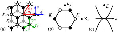
Figure 1: (a) Crystal structure of bilayer graphene. The honeycomb structure of the upper (lower) layer is marked in black (gray). Atoms in sublattices $A$ and $A^{\prime}$ ($B$ and $B^{\prime}$) are marked with open (closed) circles. (b) Brillouin zone and its two inequivalent corner points ${\bm{\mathrm{K}}}$ and ${\bm{\mathrm{K}}}^{\prime}$. The remaining corners are related with ${\bm{\mathrm{K}}}$ or ${\bm{\mathrm{K}}}^{\prime}$ by reciprocal lattice vectors. (c) Dispersion $E(k)$ near the ${\bm{\mathrm{K}}}$ point. We have ${\bm{\mathrm{k}}}\equiv\bm{\kappa}-{\bm{\mathrm{K}}}$.

The crystal structure and Brillouin zone of BLG are illustrated in Fig. 1(a) and (b), respectively. The band structure near the ${\bm{\mathrm{K}}}$ point is described by the effective Hamiltonian McCann and Fal’ko (2006); Castro Neto et al. (2009); McCann and Koshino (2013)

$$\begin{array}[b]{r>{\displaystyle}l}(\mathcal{H}^{\bm{\mathrm{K}}}_{\bm{\mathrm{k}}})_{33}({\bm{\mathrm{k}}})=&\frac{\hbar^{2}}{2m_{0}}\left[-u\left(k_{+}^{2}\,\sigma_{+}+k_{-}^{2}\,\sigma_{-}\right)+w\,k^{2}\sigma_{0}\right]\\[6.45831pt] &\hskip 60.00009pt-\,\hbar v\left(k_{-}\,\sigma_{+}+k_{+}\,\sigma_{-}\right)\;,\end{array}$$ (1)

where $\hbar$ is Planck’s constant, $m_{0}$ is the free-electron mass, ${\bm{\mathrm{k}}}\equiv(k_{x},k_{y})$ is the electrons’ wave vector measured from ${\bm{\mathrm{K}}}$, and the Pauli matrices $\sigma_{x,y,z}$ are associated with the sublattice (or, equivalently, the layer-index) pseudospin degree of freedom Castro Neto et al. (2009). In our notation, $\sigma_{0}$ is the $2\times 2$ unit matrix, $\sigma_{\pm}=(\sigma_{x}\pm i\sigma_{y})/2$, and $k_{\pm}=k_{x}\pm ik_{y}$. Numerical values for the (positive and dimensionless) prefactors $u$, $w$ and the speed $v$ are well known McCann and Fal’ko (2006); Castro Neto et al. (2009), see below. Very close to the ${\bm{\mathrm{K}}}$ point, the energy dispersion resulting from Eq. (1) mimics that of massless Dirac electrons, as is the case in single-layer graphene (SLG). However, as $u\gg w$, the dominant behavior of electrons in BLG is captured by the quadratic dispersion shown in Fig. 1(c).

External fields turn out to have a great influence on the electronic properties of charge carriers in BLG. Previously, only the effects of electric and magnetic fields directed perpendicular to the BLG sheet have been considered, which can be described by the extended effective Hamiltonian

$$\begin{array}[b]{l}\mathcal{H}^{\bm{\mathrm{K}}}_{33}({\bm{\mathrm{k}}},\mathcal{E}_{z},B_{z})=(\mathcal{H}^{\bm{\mathrm{K}}}_{\bm{\mathrm{k}}})_{33}({\bm{\mathrm{k}}})\\[2.15277pt] \hskip 20.00003pt\displaystyle{}+\frac{g_{\mathrm{e}}}{2}\,\frac{\mathcal{E}_{z}}{c}\,\mu_{\mathrm{B}}\,\sigma_{z}-\frac{g_{\mathrm{m}}}{2}\,B_{z}\,\mu_{\mathrm{B}}\,\sigma_{z}+e\,\xi_{z}\,\mathcal{E}_{z}B_{z}\,\sigma_{0}\,.\end{array}$$ (2)

Here we have followed the common practice Kittel (1963) that $\hbar{\bm{\mathrm{k}}}$ denotes both crystal momentum and, for a magnetic field $B>0$ the operator of kinetic momentum, $\hbar{\bm{\mathrm{k}}}=-i\hbar\nabla+e{\bm{\mathrm{A}}}$, the components of which obey the commutator relation $[k_{x},k_{y}]=(e/i\hbar)B_{z}$. According to Eq. (2), (i) a potential difference between the two layers (equivalent to a finite electric field $\mathcal{E}_{z}$) opens up a pseudospin gap McCann and Fal’ko (2006); McCann (2006); Ohta et al. (2006); Zhang et al. (2009) $g_{\mathrm{e}}\,\mu_{\mathrm{B}}\,\mathcal{E}_{z}/c$, (ii) a magnetic field $B_{z}$ induces a pseudospin Zeeman splitting Zhang et al. (2011) $g_{\mathrm{m}}\,\mu_{\mathrm{B}}\,B_{z}$, and (iii) the simultaneous presence of fields $\mathcal{E}_{z}$ and $B_{z}$ leads to a (valley-contrasting, see below) overall energy shift Xiao et al. (2007); Nakamura et al. (2009); Koshino and McCann (2010); Zhang et al. (2011); Zülicke and Winkler (2014), $e\,\xi_{z}\,\mathcal{E}_{z}B_{z}$. In Eq. (2), the effective g factors $g_{\mathrm{e}}$ and $g_{\mathrm{m}}$ as well as the prefactor $\xi_{z}$ are material parameters, $\mu_{\mathrm{B}}$ is the Bohr magneton, and ${\bm{\mathrm{A}}}$ is the electromagnetic vector potential satisfying $({\bm{\mathrm{\nabla}}}\times{\bm{\mathrm{A}}})_{z}=B_{z}$. The matter-field interactions (i)–(iii) generate sizable effects for typical values of $\mathcal{E}_{z}$ and $B_{z}$. As discussed in more detail below, we have $g_{\mathrm{e}}\simeq 500$, $g_{\mathrm{m}}\simeq 6.2$, and $\xi_{z}=3\times 10^{-4}~{}\mathrm{nm/T}$.

Inspection of Eq. (2) reveals a surprising feature: disregarding constant prefactors, the electron’s interaction with fields $\mathcal{E}_{z}$ and $B_{z}$ is symmetric with respect to the interchange of $\mathcal{E}_{z}$ and $B_{z}$. Indeed, this observation is not a coincidence. It reflects the unusual property of electron states near the ${\bm{\mathrm{K}}}$ point of the BLG Brillouin zone that crystal symmetry does not distinguish between polar vectors such as the electric field ${\bm{\mathcal{E}}}$ and axial vectors such as the magnetic field ${\bm{\mathrm{B}}}$. Moreover, the familiar constraints due to time-reversal invariance are modified at the BLG ${\bm{\mathrm{K}}}$ point such that symmetry under time reversal likewise permits that ${\bm{\mathcal{E}}}$ and ${\bm{\mathrm{B}}}$ become interchangeable.

In the following, we provide a rigorous derivation of the magneto-electric equivalence exhibited in BLG and discuss physical ramifications, with most of our major findings given in Secs. IV and VI. Noteworthy results include Table 3, which juxtaposes lowest-order ${\bm{\mathrm{B}}}$- and ${\bm{\mathcal{E}}}$-dependent terms in the effective Hamiltonian for electrons in BLG related by magneto-electric equivalence and elucidates their opposite symmetry with respect to the valley degree of freedom; Fig. 2, which illustrates and compares the spin and pseudospin textures induced by each of these terms in the two valleys; and Table 4, which provides parametric expressions and numerical values for prefactors. In addition, we discuss the measurable thermodynamic response induced by magnetic and electric fields in BLG, which turns out to be completely symmetric under exchange of ${\bm{\mathrm{B}}}$ and ${\bm{\mathcal{E}}}$, see Eqs. (24) and (26). These features reveal unconventional behavior of spin and pseudospin degrees of freedom induced by external fields. Although seemingly counterintuitive, our findings are consistent with fundamental principles such as time reversal symmetry. This is indicated, e.g., by the fact that only a magnetic field $B_{z}$ can give rise to a macroscopic polarization of the real spin $s_{z}$, whereas only an electric field $\mathcal{E}_{z}$ can induce a macroscopic polarization of the pseudospin $\sigma_{z}$. These symmetry-enforced rules for the matter-field interactions can serve to distinguish the physical nature of spins versus pseudospins.

Our paper is organized as follows. To establish some important notations and conventions, we start in Sec. II with a brief review of results previously obtained for BLG within a tight-binding analysis. The basic formalism and results from the invariant expansion for the BLG band structure near the ${\bm{\mathrm{K}}}$ point are given in Sec. III. It reveals the magneto-electric equivalence, which is analyzed in greater detail in Sec. IV. To develop a more quantitative description of the predicted effects, we apply the theory of invariants in Sec. V to extend the tight-binding model from Sec. II to include spin-orbit coupling and the effect of external magnetic and electric fields. This extended model is then analyzed in Sec. VI by means of Löwdin partitioning in order to derive explicit expressions for the prefactors of the terms describing the magneto-electric equivalence in BLG. We finish by drawing conclusions in Sec. VII.

II Review of Tight-Binding Analysis

In this section we present a brief review of results previously obtained for BLG within a tight-binding analysis. This enables us to establish some important notations and conventions. Also, it allows us to properly relate our findings to previous work.

The crystal structure of BLG is sketched in Fig. 1(a). For definiteness, we use the basis vectors in real space

$${\bm{\mathrm{a}}}_{1}=a\left(\begin{array}[]{s{0.15em}cs{0.15em}}\hskip 1.49994pt\lx@intercol\hfil 1\hfil\hskip 1.49994pt\\ \hskip 1.49994pt\lx@intercol\hfil 0\hfil\hskip 1.49994pt\\ \hskip 1.49994pt\lx@intercol\hfil 0\hfil\hskip 1.49994pt\end{array}\right),\qquad{\bm{\mathrm{a}}}_{2}=a\left(\begin{array}[]{s{0.15em}cs{0.15em}}\hskip 1.49994pt\lx@intercol\hfil 1/2\hfil\hskip 1.49994pt\\ \hskip 1.49994pt\lx@intercol\hfil\sqrt{3}/2\hfil\hskip 1.49994pt\\ \hskip 1.49994pt\lx@intercol\hfil 0\hfil\hskip 1.49994pt\end{array}\right),\qquad{\bm{\mathrm{a}}}_{3}=\left(\begin{array}[]{s{0.15em}cs{0.15em}}\hskip 1.49994pt\lx@intercol\hfil 0\hfil\hskip 1.49994pt\\ \hskip 1.49994pt\lx@intercol\hfil 0\hfil\hskip 1.49994pt\\ \hskip 1.49994pt\lx@intercol\hfil c\hfil\hskip 1.49994pt\end{array}\right),$$ (3)

with lattice constants $a$ and $c$. The two inequivalent corner points of the 2D Brillouin zone are then

$${\bm{\mathrm{K}}}=\frac{2\pi}{a}\left(\begin{array}[]{s{0.15em}cs{0.15em}}\hskip 1.49994pt\lx@intercol\hfil 2/3\hfil\hskip 1.49994pt\\ \hskip 1.49994pt\lx@intercol\hfil 0\hfil\hskip 1.49994pt\end{array}\right),\quad{\bm{\mathrm{K}}}^{\prime}=\frac{2\pi}{a}\left(\begin{array}[]{s{0.15em}cs{0.15em}}\hskip 1.49994pt\lx@intercol\hfil-2/3\hfil\hskip 1.49994pt\\ \hskip 1.49994pt\lx@intercol\hfil 0\hfil\hskip 1.49994pt\end{array}\right).$$ (4)

We consider a tight-binding Hamiltonian for the BLG $\pi$ bonds formed by the carbon $p_{z}$ orbitals, taking into account nearest-neighbor and second-nearest-neighbor interactions in-plane and out-of-plane. For a given atom in a honeycomb layer, the vectors connecting nearest-neighbor atoms are ($j=1,2,3$)

$${\bm{\mathrm{\tau}}}^{(j)}_{1}=\mathcal{R}(2j\pi/3)\,{\bm{\mathrm{\tau}}}^{(3)}_{1},\quad{\bm{\mathrm{\tau}}}^{(3)}_{1}=a\left(\begin{array}[]{s{0.15em}cs{0.15em}}\hskip 1.49994pt\lx@intercol\hfil 0\hfil\hskip 1.49994pt\\ \hskip 1.49994pt\lx@intercol\hfil 1/\sqrt{3}\hfil\hskip 1.49994pt\\ \hskip 1.49994pt\lx@intercol\hfil 0\hfil\hskip 1.49994pt\end{array}\right),$$ (5)

where $\mathcal{R}(\phi)$ denotes a 2D rotation in the $xy$ plane by the angle $\phi$. Similarly, we get the vectors connecting second-nearest-neighbor atoms ($j=1,\ldots,6$)

$${\bm{\mathrm{\tau}}}^{(j)}_{2}=\mathcal{R}(j\,\pi/3)\,{\bm{\mathrm{a}}}_{1}.$$ (6)

Then the tight-binding Hamiltonian becomes (in the order $A$, $B$, $A^{\prime}$, $B^{\prime}$) Wallace (1947)

$$\begin{array}[b]{@{}l@{}}\mathcal{H}(\bm{\kappa})=\tilde{E}_{0}+\gamma_{0}^{\prime}f_{2}\\[4.30554pt] \hskip 10.00002pt+\left(\begin{array}[]{s{0.15em}ccccs{0.15em}}\hskip 1.49994pt\lx@intercol\hfil\Delta&-\gamma_{0}\,f_{1}&\gamma_{1}&\gamma_{4}f_{1}^{\ast}\hfil\hskip 1.49994pt\\[6.45831pt] \hskip 1.49994pt\lx@intercol\hfil-\gamma_{0}\,f_{1}^{\ast}&0&\gamma_{4}f_{1}^{\ast}&\gamma_{3}f_{1}\hfil\hskip 1.49994pt\\[6.45831pt] \hskip 1.49994pt\lx@intercol\hfil\gamma_{1}&\gamma_{4}f_{1}&\Delta&-\gamma_{0}\,f_{1}^{\ast}\hfil\hskip 1.49994pt\\[6.45831pt] \hskip 1.49994pt\lx@intercol\hfil\gamma_{4}f_{1}&\gamma_{3}f_{1}^{\ast}&-\gamma_{0}\,f_{1}&0\hfil\hskip 1.49994pt\end{array}\right),\end{array}$$ (7)

where $\tilde{E}_{0}$ is the site energy of the $p_{z}$ orbitals, $\Delta$ denotes the difference between the site energies of $A$ atoms compared with $B$ atoms, $\gamma_{0}$ ($\gamma_{0}^{\prime}$) is the transfer integral for nearest (second-nearest) neighbors within each layer, and $\gamma_{1}$, $\gamma_{3}$, and $\gamma_{4}$ are transfer integrals for atoms in neighboring layers. The functions $f_{l}(\bm{\kappa})$ are given by

$$f_{l}(\bm{\kappa})\equiv\sum_{j}e^{i\bm{\kappa}\cdot{\bm{\mathrm{\tau}}}^{(j)}_{l}}.$$ (8)

The particular geometry (5) gives for $f_{1}(\bm{\kappa})$

$$f_{1}(\bm{\kappa})=e^{i\kappa_{y}a/\sqrt{3}}+2e^{-i\kappa_{y}a/2\sqrt{3}}\cos(\kappa_{x}a/2),$$ (9)

and we have the relation

$$f_{2}(\bm{\kappa})=|f_{1}(\bm{\kappa})|^{2}-3.$$ (10)

Thus it is possible to rewrite the Hamiltonian (7) such that it only depends on the function $f_{1}$. Also, we rearrange the basis functions in the order $\frac{1}{\sqrt{2}}(A+A^{\prime})$, $\frac{1}{\sqrt{2}}(A-A^{\prime})$, $B$, $B^{\prime}$ giving

$$\mathcal{H}(\bm{\kappa})=E_{0}+\gamma_{0}^{\prime}f_{1}^{2}+\left(\begin{array}[]{s{0.15em}ccccs{0.15em}}\hskip 1.49994pt\lx@intercol\hfil\Delta+\gamma_{1}&0&{\textstyle\frac{1}{\sqrt{2}}}(-\gamma_{0}+\gamma_{4})f_{1}&{\textstyle\frac{1}{\sqrt{2}}}(-\gamma_{0}+\gamma_{4})f_{1}^{\ast}\hfil\hskip 1.49994pt\\[6.45831pt] \hskip 1.49994pt\lx@intercol\hfil 0&\Delta-\gamma_{1}&-{\textstyle\frac{1}{\sqrt{2}}}(\gamma_{0}+\gamma_{4})f_{1}&{\textstyle\frac{1}{\sqrt{2}}}(\gamma_{0}+\gamma_{4})f_{1}^{\ast}\hfil\hskip 1.49994pt\\[6.45831pt] \hskip 1.49994pt\lx@intercol\hfil{\textstyle\frac{1}{\sqrt{2}}}(-\gamma_{0}+\gamma_{4})f_{1}^{\ast}&-{\textstyle\frac{1}{\sqrt{2}}}(\gamma_{0}+\gamma_{4})f_{1}^{\ast}&0&\gamma_{3}f_{1}\hfil\hskip 1.49994pt\\[6.45831pt] \hskip 1.49994pt\lx@intercol\hfil{\textstyle\frac{1}{\sqrt{2}}}(-\gamma_{0}+\gamma_{4})f_{1}&{\textstyle\frac{1}{\sqrt{2}}}(\gamma_{0}+\gamma_{4})f_{1}&\gamma_{3}f_{1}^{\ast}&0\hfil\hskip 1.49994pt\end{array}\right),$$ (11)

where $E_{0}=\tilde{E}_{0}-3\gamma_{0}^{\prime}$. In the following, we will neglect the constant $E_{0}$ as well as the small parameter $\Delta$. The latter approximation helps to keep formulas derived later on more readable. Next we expand $f_{1}({\bm{\mathcal{\kappa}}})=f_{1}({\bm{\mathrm{K}}}+{\bm{\mathrm{k}}})$ around the ${\bm{\mathrm{K}}}$ point. Using the coordinate system in Fig. 1 we obtain

$$f_{1}({\bm{\mathrm{k}}})=-\frac{\sqrt{3}a}{2}k_{-}+\frac{a^{2}}{4}k_{+}^{2}+\ldots\quad.$$ (12)

Substituting this into Eq. (11) gives the Slonczewski-Weiss-McClure (SWM) Hamiltonian McClure (1957)

$$\mathcal{H}^{\bm{\mathrm{K}}}_{\bm{\mathrm{k}}}({\bm{\mathrm{k}}})=\left(\begin{array}[]{s{0.15em}ccccs{0.15em}}\hskip 1.49994pt\lx@intercol\hfil\gamma_{1}+\tilde{\gamma}_{0}^{\prime}k^{2}&0&{\textstyle\frac{1}{\sqrt{2}}}(\tilde{\gamma}_{0}-\tilde{\gamma}_{4})k_{-}&{\textstyle\frac{1}{\sqrt{2}}}(\tilde{\gamma}_{0}-\tilde{\gamma}_{4})k_{+}\hfil\hskip 1.49994pt\\[6.45831pt] \hskip 1.49994pt\lx@intercol\hfil 0&-\gamma_{1}+\tilde{\gamma}_{0}^{\prime}k^{2}&{\textstyle\frac{1}{\sqrt{2}}}(\tilde{\gamma}_{0}+\tilde{\gamma}_{4})k_{-}&-{\textstyle\frac{1}{\sqrt{2}}}(\tilde{\gamma}_{0}+\tilde{\gamma}_{4})k_{+}\hfil\hskip 1.49994pt\\[6.45831pt] \hskip 1.49994pt\lx@intercol\hfil{\textstyle\frac{1}{\sqrt{2}}}(\tilde{\gamma}_{0}-\tilde{\gamma}_{4})k_{+}&{\textstyle\frac{1}{\sqrt{2}}}(\tilde{\gamma}_{0}+\tilde{\gamma}_{4})k_{+}&\tilde{\gamma}_{0}^{\prime}k^{2}&-\tilde{\gamma}_{31}k_{-}+\tilde{\gamma}_{32}k_{+}^{2}\hfil\hskip 1.49994pt\\[6.45831pt] \hskip 1.49994pt\lx@intercol\hfil{\textstyle\frac{1}{\sqrt{2}}}(\tilde{\gamma}_{0}-\tilde{\gamma}_{4})k_{-}&-{\textstyle\frac{1}{\sqrt{2}}}(\tilde{\gamma}_{0}+\tilde{\gamma}_{4})k_{-}&-\tilde{\gamma}_{31}k_{+}+\tilde{\gamma}_{32}k_{-}^{2}&\tilde{\gamma}_{0}^{\prime}k^{2}\hfil\hskip 1.49994pt\end{array}\right).$$ (13)

Here $(\mathcal{H}^{\bm{\mathrm{K}}}_{\bm{\mathrm{k}}})_{11}$ describes the uppermost band at the ${\bm{\mathrm{K}}}$ point transforming according to the irreducible representation $\Gamma_{1}$ of $D_{3}$ (we follow the notation of Koster et al. Koster et al. (1963)), $(\mathcal{H}^{\bm{\mathrm{K}}}_{\bm{\mathrm{k}}})_{22}$ corresponds to the lowest band transforming according to $\Gamma_{2}$ of $D_{3}$, and the lower right $2\times 2$ block corresponds to a band transforming according to $\Gamma_{3}$ of $D_{3}$ which is two-fold degenerate at the ${\bm{\mathrm{K}}}$ point. We have

$$\begin{array}[b]{rcl*{2}{s{1em}rcl}}\tilde{\gamma}_{0}&\equiv&{\textstyle\frac{\sqrt{3}a}{2}}\gamma_{0},\hfil\hskip 10.00002pt&\tilde{\gamma}_{0}^{\prime}&\equiv&{\textstyle\frac{3a^{2}}{4}}\gamma_{0}^{\prime},\hfil\hskip 10.00002pt\\[8.61108pt] \tilde{\gamma}_{31}&\equiv&{\textstyle\frac{\sqrt{3}a}{2}}\gamma_{3},\hfil\hskip 10.00002pt&\tilde{\gamma}_{32}&\equiv&{\textstyle\frac{a^{2}}{4}}\gamma_{3},\hfil\hskip 10.00002pt&\tilde{\gamma}_{4}&\equiv&{\textstyle\frac{\sqrt{3}a}{2}}\gamma_{4}.\end{array}$$ (14)

Projecting $\mathcal{H}({\bm{\mathrm{k}}})$ on the $\Gamma_{3}$ subspace using quasi-degenerate perturbation theory Bir and Pikus (1974); Winkler (2003) gives in lowest order the effective $2\times 2$ Hamiltonian [cf. Eq. (2)]

$$\begin{array}[b]{r>{\displaystyle}l}(\mathcal{H}^{\bm{\mathrm{K}}}_{\bm{\mathrm{k}}})_{33}({\bm{\mathrm{k}}})=&\frac{\hbar^{2}}{2m_{0}}\left[-u\left(k_{+}^{2}\,\sigma_{+}+k_{-}^{2}\,\sigma_{-}\right)+w\,k^{2}\sigma_{0}\right]\\[6.45831pt] &-\hbar v\left(k_{-}\,\sigma_{+}+k_{+}\,\sigma_{-}\right)-\frac{g_{\mathrm{m}}}{2}\,\mu_{\mathrm{B}}\,B_{z}\,\sigma_{z}\;.\end{array}$$ (15)

[To also obtain the $\mathcal{E}_{z}$-dependent terms in Eq. (2) that are absent in Eq. (15), a more refined analysis is required, see Sec. VI below.] Defining the energy scale

$$\gamma_{a}=\frac{2\hbar^{2}}{3m_{0}a^{2}}\approx 0.85~{}\mathrm{eV}\;,$$ (16a)

we can express the new parameters in terms of the tight-binding parameters as follows:

$$u =\frac{\gamma_{0}^{2}+\gamma_{4}^{2}-\gamma_{1}\gamma_{3}/3}{\gamma_{1}\gamma_{a}} \approx 33\quad,$$ (16b)

$$w =\frac{\gamma_{0}^{\prime}\gamma_{1}+2\gamma_{0}\gamma_{4}}{\gamma_{1}\gamma_{a}} \approx 3.4\quad,$$ (16c)

$$v =\frac{\tilde{\gamma}_{31}}{\hbar}={\textstyle\frac{\sqrt{3}a}{2\hbar}}\gamma_{3} \approx 8.1\times 10^{4}~{}\mathrm{m\,s^{-1}}\quad,$$ (16d)

$$g_{\mathrm{m}} =\frac{4\gamma_{0}\gamma_{4}}{\gamma_{1}\gamma_{a}} \approx 6.2\quad.$$ (16e)

Here we assumed $\gamma_{0}=3.0$ eV, $\gamma_{0}^{\prime}=0.22$ eV, $\gamma_{4}=0.14$ eV, $\gamma_{1}=0.32$ eV, $\gamma_{3}=0.25$ eV, and $a=0.245$ nm.

III Symmetry analysis and invariant expansion for BLG

The SWM-like Hamiltonians (13) and (15) give the band structure of BLG as a function of the wave vector ${\bm{\mathrm{k}}}$ measured from the ${\bm{\mathrm{K}}}$ point. The theory of invariants Bir and Pikus (1974); Winkler and Zülicke (2010) allows one to generalize these results to perturbations ${\bm{\mathcal{K}}}$ that involve combinations of various quantities in addition to the wave vector ${\bm{\mathrm{k}}}$, e.g., electric and magnetic fields ${\bm{\mathcal{E}}}$ and ${\bm{\mathrm{B}}}$, strain ${\bm{\mathrm{\epsilon}}}$ and the intrinsic spin ${\bm{\mathrm{s}}}$. The group of the wave vector ${\bm{\mathrm{K}}}$ is isomorphic to the trigonal point group $D_{3}$ so that we can classify the electronic states near ${\bm{\mathrm{K}}}$ using the irreducible representations of $D_{3}$ Koster et al. (1963). The $4\times 4$ Hamiltonian $\mathcal{H}^{\bm{\mathrm{K}}}$ falls into blocks

$$\mathcal{H}^{\bm{\mathrm{K}}}=\left(\begin{array}[]{s{0.15em}cccs{0.15em}}\hskip 1.49994pt\lx@intercol\hfil\mathcal{H}_{11}&\mathcal{H}_{12}&\mathcal{H}_{13}\hfil\hskip 1.49994pt\\ \hskip 1.49994pt\lx@intercol\hfil\mathcal{H}_{21}&\mathcal{H}_{22}&\mathcal{H}_{23}\hfil\hskip 1.49994pt\\ \hskip 1.49994pt\lx@intercol\hfil\mathcal{H}_{31}&\mathcal{H}_{32}&\mathcal{H}_{33}\hfil\hskip 1.49994pt\end{array}\right),$$ (17)

where each diagonal block $\mathcal{H}_{\alpha\alpha}$ describes a band transforming according to the irreducible representation $\Gamma_{\alpha}$ of $D_{3}$. In the end, we are mainly interested in the block $\mathcal{H}_{33}$ corresponding to the highest valence band and lowest conduction band of BLG. However, for the study of prefactors given in Sec. VI, all bands in the SWM model are included.

According to the theory of invariants, each block $\mathcal{H}_{\alpha\beta}$ takes the form

$$\mathcal{H}_{\alpha\beta}({\bm{\mathcal{K}}})=\sum_{\kappa,\,\lambda}a^{\alpha\beta}_{\kappa\lambda}\sum_{l=1}^{L_{\kappa}}{X}_{l}^{(\kappa,\alpha\beta)}\mathcal{K}_{l}^{(\kappa,\lambda)\,\ast}\,.$$ (18)

Here $a^{\alpha\beta}_{\kappa\lambda}$ are prefactors, ${X}_{l}^{(\kappa,\alpha\beta)}$ are matrices that transform according to the IRs $\Gamma_{\kappa}$ (of dimension $L_{\kappa}$) contained in the product representation $\Gamma_{\alpha}\times\Gamma_{\beta}^{\ast}$ of $D_{3}$. Likewise, ${\bm{\mathcal{K}}}$ can be decomposed into irreducible tensor operators ${\bm{\mathcal{K}}}^{(\kappa,\lambda)}$ that transform according to the IRs $\Gamma_{\kappa}$ of $D_{3}$. Using the coordinate system in Fig. 1 we obtain the basis matrices and tensor operators listed in Tables 1 and 2. For completeness, Table 2 also includes the lowest-order tensor operators due to strain. However, in the following, these strain tensor operators are not considered further. Quite generally, each term proportional to the components of the strain tensor $\epsilon_{ij}$ is formally equivalent to a term where $\epsilon_{ij}$ is replaced by the symmetrized product $\{k_{i},k_{j}\}$ Bir and Pikus (1974).

Table 1: Symmetrized matrices for the invariant expansion of the blocks $\mathcal{H}_{\alpha\beta}$ for the point group $D_{3}$.

$\begin{array}[]{clcl}\hline\cr\hline\cr\mbox{Block}&\lx@intercol\mbox{Representations}\hfil\lx@intercol&\lx@intercol\hfil\mbox{Symmetrized matrices}\hfil\lx@intercol\\ \hline\cr\mathcal{H}_{11}&\Gamma_{1}\times\Gamma_{1}^{\ast}=\Gamma_{1}&\Gamma_{1}:&(1)\\ \mathcal{H}_{22}&\Gamma_{2}\times\Gamma_{2}^{\ast}=\Gamma_{1}&\Gamma_{1}:&(1)\\ \mathcal{H}_{12}&\Gamma_{1}\times\Gamma_{2}^{\ast}=\Gamma_{2}&\Gamma_{2}:&(1)\\ \mathcal{H}_{13}&\Gamma_{1}\times\Gamma_{3}^{\ast}=\Gamma_{3}&\Gamma_{3}:&(1,1),(-i,i)\\ \mathcal{H}_{23}&\Gamma_{2}\times\Gamma_{3}^{\ast}=\Gamma_{3}&\Gamma_{3}:&(1,-1),(-i,-i)\\ \mathcal{H}_{33}&\Gamma_{3}\times\Gamma_{3}^{\ast}&\Gamma_{1}:&\openone\\ &=\Gamma_{1}+\Gamma_{2}+\Gamma_{3}&\Gamma_{2}:&\sigma_{z}\\ &&\Gamma_{3}:&\sigma_{x},\sigma_{y}\\ \hline\cr\hline\cr\end{array}$

Table 2: Irreducible tensor components for the point group $D_{3}$ (the group of the ${\bm{\mathrm{K}}}$ point in BLG). Terms printed in bold give rise to invariants in the block $\mathcal{H}^{\bm{\mathrm{K}}}_{33}$ allowed by time-reversal invariance. (No terms proportional to $k_{z}$ are listed as they are irrelevant for graphene.) Contributions that are new in BLG (i.e., are not part of the corresponding set Winkler and Zülicke (2010) for $D_{3h}$ which is the group of the ${\bm{\mathrm{K}}}$ point in SLG) are marked by $\ddagger$. Notation: $\{A,B\}\equiv\frac{1}{2}(AB+BA)$.

$\begin{array}[]{cs{1.0em}p{0.9\columnwidth}}\hline\cr\hline\cr\Gamma_{1}\hfil\hskip 10.00002pt&\mbox{$\bm{1}$}; \mbox{$\bm{k_{x}^{2}+k_{y}^{2}}$}; \mbox{$\bm{\{k_{x},3k_{y}^{2}-k_{x}^{2}\}}$}; \mbox{$B_{x}k_{x}+B_{y}k_{y}$}; \newline \mbox{$k_{x}\mathcal{E}_{x}+k_{y}\mathcal{E}_{y}$}; \mbox{$\bm{\mathcal{E}_{x}B_{x}+\mathcal{E}_{y}B_{y}}$}$\ddagger$; \mbox{$\bm{\mathcal{E}_{z}B_{z}}$}$\ddagger$; \mbox{$\bm{\epsilon_{xx}+\epsilon_{yy}}$}; \mbox{$\bm{\epsilon_{zz}}$}$\ddagger$; \newline \mbox{$\bm{(\epsilon_{yy}-\epsilon_{xx})k_{x}+2\epsilon_{xy}k_{y}}$}; \mbox{$\bm{\epsilon_{yz}k_{x}-\epsilon_{xz}k_{y}}$}$\ddagger$; \newline \mbox{$(\epsilon_{yy}-\epsilon_{xx})B_{x}+2\epsilon_{xy}B_{y}$}; \mbox{$\epsilon_{yz}B_{x}-\epsilon_{xz}B_{y}$}; \newline \mbox{$(\epsilon_{yy}-\epsilon_{xx})\mathcal{E}_{x}+2\epsilon_{xy}\mathcal{E}_{y}$}; \mbox{$\epsilon_{yz}\mathcal{E}_{x}-\epsilon_{xz}\mathcal{E}_{y}$}; \mbox{$s_{x}k_{x}+s_{y}k_{y}$}; \newline \mbox{$\bm{s_{x}B_{x}+s_{y}B_{y}}$}; \mbox{$\bm{s_{z}B_{z}}$}; \mbox{$\bm{s_{x}\mathcal{E}_{x}+s_{y}\mathcal{E}_{y}}$}$\ddagger$; \mbox{$\bm{s_{z}\mathcal{E}_{z}}$}$\ddagger$; \newline \mbox{$\bm{(s_{x}k_{y}-s_{y}k_{x})\mathcal{E}_{z}}$}; \mbox{$\bm{s_{z}(k_{x}\mathcal{E}_{y}-k_{y}\mathcal{E}_{x})}$}; \newline \mbox{$s_{x}(\epsilon_{yy}-\epsilon_{xx})+2s_{y}\epsilon_{xy}$}; \mbox{$s_{x}\epsilon_{yz}-s_{y}\epsilon_{xz}$}\\ \Gamma_{2}\hfil\hskip 10.00002pt&\mbox{$\{k_{y},3k_{x}^{2}-k_{y}^{2}\}$}; \mbox{$\bm{B_{z}}$}; \mbox{$\bm{k_{x}B_{y}-k_{y}B_{x}}$}$\ddagger$; \mbox{$\bm{\mathcal{E}_{z}}$}$\ddagger$; \mbox{$\bm{k_{x}\mathcal{E}_{y}-k_{y}\mathcal{E}_{x}}$}; \newline \mbox{$\mathcal{E}_{x}B_{y}-\mathcal{E}_{y}B_{x}$}; \mbox{$(\epsilon_{xx}-\epsilon_{yy})k_{y}+2\epsilon_{xy}k_{x}$}; \mbox{$\epsilon_{yz}k_{y}+\epsilon_{xz}k_{x}$}; \newline \mbox{$\bm{(\epsilon_{xx}-\epsilon_{yy})B_{y}+2\epsilon_{xy}B_{x}}$}$\ddagger$; \mbox{$\bm{(\epsilon_{xx}+\epsilon_{yy})B_{z}}$}; \mbox{$\bm{\epsilon_{zz}B_{z}}$}$\ddagger$; \newline \mbox{$\bm{\epsilon_{xz}B_{x}+\epsilon_{yz}B_{y}}$}$\ddagger$; \mbox{$\bm{(\epsilon_{xx}-\epsilon_{yy})\mathcal{E}_{y}+2\epsilon_{xy}\mathcal{E}_{x}}$}; \newline \mbox{$\bm{(\epsilon_{xx}+\epsilon_{yy})\mathcal{E}_{z}}$}$\ddagger$; \mbox{$\bm{\epsilon_{zz}\mathcal{E}_{z}}$}$\ddagger$; \mbox{$\bm{\epsilon_{xz}\mathcal{E}_{x}+\epsilon_{yz}\mathcal{E}_{y}}$}$\ddagger$; \mbox{$\bm{s_{z}}$}; \newline \mbox{$\bm{s_{x}k_{y}-s_{y}k_{x}}$}$\ddagger$; \mbox{$s_{x}B_{y}-s_{y}B_{x}$}; \mbox{$s_{x}\mathcal{E}_{y}-s_{y}\mathcal{E}_{x}$}; \newline \mbox{$(s_{x}k_{x}+s_{y}k_{y})\mathcal{E}_{z}$}; \mbox{$\bm{s_{y}(\epsilon_{xx}-\epsilon_{yy})+2s_{x}\epsilon_{xy}}$}$\ddagger$;\newline \mbox{$\bm{s_{z}(\epsilon_{xx}+\epsilon_{yy})}$}; \mbox{$\bm{s_{x}\epsilon_{xz}+s_{y}\epsilon_{yz}}$}$\ddagger$; \mbox{$\bm{s_{z}\epsilon_{zz}}$}$\ddagger$;\\ \Gamma_{3}\hfil\hskip 10.00002pt&\mbox{$\bm{k_{x},k_{y}}$}; \mbox{$\bm{\{k_{y}+k_{x},k_{y}-k_{x}\},2\{k_{x},k_{y}\}}$}; \newline \mbox{$\bm{\{k_{x},k_{x}^{2}+k_{y}^{2}\},\{k_{y},k_{x}^{2}+k_{y}^{2}\}}$}; \newline \mbox{$B_{x},B_{y}$}; \mbox{$B_{y}k_{y}-B_{x}k_{x},B_{x}k_{y}+B_{y}k_{x}$}; \mbox{$B_{z}k_{y},-B_{z}k_{x}$}; \newline \mbox{$\mathcal{E}_{x},\mathcal{E}_{y}$}; \mbox{$\mathcal{E}_{y}k_{y}-\mathcal{E}_{x}k_{x},\mathcal{E}_{x}k_{y}+\mathcal{E}_{y}k_{x}$}; \mbox{$\mathcal{E}_{z}k_{y},-\mathcal{E}_{z}k_{x}$}; \newline \mbox{$\bm{\mathcal{E}_{y}B_{y}-\mathcal{E}_{x}B_{x},\mathcal{E}_{y}B_{x}+\mathcal{E}_{x}B_{y}}$}$\ddagger$; \mbox{$\bm{\mathcal{E}_{y}B_{z},-\mathcal{E}_{x}B_{z}}$}; \newline \mbox{$\bm{\mathcal{E}_{z}B_{y},-\mathcal{E}_{z}B_{x}}$}; \mbox{$\bm{\epsilon_{yy}-\epsilon_{xx},2\epsilon_{xy}}$}; \mbox{$\bm{\epsilon_{yz},-\epsilon_{xz}}$}$\ddagger$; \newline \mbox{$\bm{(\epsilon_{xx}+\epsilon_{yy})(k_{x},k_{y})}$}; \mbox{$\bm{\epsilon_{yz}k_{x}+\epsilon_{xz}k_{y},\epsilon_{xz}k_{x}-\epsilon_{yz}k_{y}}$}$\ddagger$; \newline \mbox{$\bm{(\epsilon_{xx}-\epsilon_{yy})k_{x}+2\epsilon_{xy}k_{y},(\epsilon_{yy}-\epsilon_{xx})k_{y}+2\epsilon_{xy}k_{x}}$}; \newline \mbox{$\bm{\epsilon_{zz}k_{x},\epsilon_{zz}k_{y}}$}$\ddagger$; \newline \mbox{$(\epsilon_{xx}+\epsilon_{yy})(B_{x},B_{y})$}; \mbox{$\epsilon_{yz}B_{x}+\epsilon_{xz}B_{y},\epsilon_{xz}B_{x}-\epsilon_{yz}B_{y}$}; \newline \mbox{$(\epsilon_{xx}-\epsilon_{yy})B_{x}+2\epsilon_{xy}B_{y},(\epsilon_{yy}-\epsilon_{xx})B_{y}+2\epsilon_{xy}B_{x}$}; \newline \mbox{$2\epsilon_{xy}B_{z},(\epsilon_{xx}-\epsilon_{yy})B_{z}$}; \mbox{$\epsilon_{zz}B_{x},\epsilon_{zz}B_{y}$}; \mbox{$\epsilon_{xz}B_{z},\epsilon_{yz}B_{z}$}; \newline \mbox{$(\epsilon_{xx}+\epsilon_{yy})(\mathcal{E}_{x},\mathcal{E}_{y})$}; \mbox{$\epsilon_{yz}\mathcal{E}_{x}+\epsilon_{xz}\mathcal{E}_{y},\epsilon_{xz}\mathcal{E}_{x}-\epsilon_{yz}\mathcal{E}_{y}$}; \newline \mbox{$(\epsilon_{xx}-\epsilon_{yy})\mathcal{E}_{x}+2\epsilon_{xy}\mathcal{E}_{y},(\epsilon_{yy}-\epsilon_{xx})\mathcal{E}_{y}+2\epsilon_{xy}\mathcal{E}_{x}$}; \newline \mbox{$2\epsilon_{xy}\mathcal{E}_{z},(\epsilon_{xx}-\epsilon_{yy})\mathcal{E}_{z}$}; \mbox{$\epsilon_{zz}\mathcal{E}_{x},\epsilon_{zz}\mathcal{E}_{y}$}; \mbox{$\epsilon_{xz}\mathcal{E}_{z},\epsilon_{yz}\mathcal{E}_{z}$}; \newline \mbox{$s_{x},s_{y}$}; \mbox{$s_{y}k_{y}-s_{x}k_{x},s_{x}k_{y}+s_{y}k_{x}$}; \mbox{$s_{z}k_{y},-s_{z}k_{x}$}; \newline \mbox{$\bm{s_{y}B_{y}-s_{x}B_{x},s_{x}B_{y}+s_{y}B_{x}}$}; \mbox{$\bm{s_{z}B_{y},-s_{z}B_{x}}$}$\ddagger$; \newline \mbox{$\bm{s_{y}B_{z},-s_{x}B_{z}}$}$\ddagger$; \mbox{$\bm{s_{y}\mathcal{E}_{y}-s_{x}\mathcal{E}_{x},s_{x}\mathcal{E}_{y}+s_{y}\mathcal{E}_{x}}$}$\ddagger$; \newline \mbox{$\bm{s_{z}\mathcal{E}_{y},-s_{z}\mathcal{E}_{x}}$}; \mbox{$\bm{s_{y}\mathcal{E}_{z},-s_{x}\mathcal{E}_{z}}$}; \newline \mbox{$\bm{s_{z}(k_{x}\mathcal{E}_{y}+k_{y}\mathcal{E}_{x}),s_{z}(k_{x}\mathcal{E}_{x}-k_{y}\mathcal{E}_{y})}$}; \newline \mbox{$\bm{(k_{x},k_{y})s_{z}\mathcal{E}_{z}}$}$\ddagger$; \mbox{$\bm{(s_{x}k_{y}+s_{y}k_{x},s_{x}k_{x}-s_{y}k_{y})\mathcal{E}_{z}}$}; \newline \mbox{$(s_{x},s_{y})(\epsilon_{xx}+\epsilon_{yy})$}; \mbox{$2s_{z}\epsilon_{xy},s_{z}(\epsilon_{xx}-\epsilon_{yy})$}; \newline \mbox{$s_{x}(\epsilon_{xx}-\epsilon_{yy})-2s_{y}\epsilon_{xy},s_{y}(\epsilon_{yy}-\epsilon_{xx})-2s_{x}\epsilon_{xy}$}; \newline \mbox{$s_{x}\epsilon_{zz},s_{y}\epsilon_{zz}$}; \mbox{$s_{z}\epsilon_{xz},s_{z}\epsilon_{yz}$}; \mbox{$s_{x}\epsilon_{yz}+s_{y}\epsilon_{xz},s_{x}\epsilon_{xz}-s_{y}\epsilon_{yz}$};\\ \hline\cr\hline\cr\end{array}$

Additional constraints for the Hamiltonian (17) are due to time reversal invariance. The crystallographic point group $D_{3d}$ of BLG contains symmetry elements $R$ mapping the basis functions $\Psi_{{\bm{\mathrm{K}}}\lambda}$ at ${\bm{\mathrm{K}}}$ on $\Psi_{{\bm{\mathrm{K}}}^{\prime}\lambda}$ at ${\bm{\mathrm{K}}}^{\prime}$. These basis functions are also mapped onto each other by time reversal $\theta$, i.e., we have

$$\theta\,\Psi_{{\bm{\mathrm{K}}},\lambda}=\Psi_{{\bm{\mathrm{K}}}\lambda}^{\ast}=\sum_{\lambda^{\prime}}\mathcal{T}_{\lambda\lambda^{\prime}}\>\Psi_{{\bm{\mathrm{K}}}^{\prime}\lambda^{\prime}}\,,$$ (19)

with a unitary matrix $\mathcal{T}$. Combining these operations we obtain Bir and Pikus (1974); Winkler and Zülicke (2010); Mañes et al. (2007)

$$\mathcal{T}^{-1}\mathcal{H}(R^{-1}{\bm{\mathcal{K}}})\mathcal{T}=\mathcal{H}^{\ast}(\zeta{\bm{\mathcal{K}}})=\mathcal{H}^{t}(\zeta{\bm{\mathcal{K}}})\,,$$ (20)

where $\ast$ denotes complex conjugation and $t$ is transposition. The quantity $\zeta$ depends on the behavior of ${\bm{\mathcal{K}}}$ under time reversal. The vectors ${\bm{\mathrm{k}}}$, ${\bm{\mathrm{B}}}$, and ${\bm{\mathrm{s}}}$ are odd under time reversal so that then $\zeta=-1$, while ${\bm{\mathcal{E}}}$ and ${\bm{\mathrm{\epsilon}}}$ have $\zeta=+1$. Equation (20) provides a general criterion for determining which terms in the expansion (18) are allowed by time-reversal invariance and which terms are forbidden. For off-diagonal blocks $\mathcal{H}_{\alpha\beta}$, the criterion (20) also determines the phase of the respective prefactors $a^{\alpha\beta}_{\kappa\lambda}$. The matrix $\mathcal{T}$ depends on the choice for the operation $R$. If $R$ is the reflection $R_{y}$ at the $yz$ plane [thus mapping the atoms in each sublattice in each layer onto each other, see Fig. 1(a)], the matrix $\mathcal{T}$ is simply the identity matrix and we obtain

$$\mathcal{H}^{\bm{\mathrm{K}}}(R_{y}^{-1}{\bm{\mathcal{K}}})=\mathcal{H}^{{\bm{\mathrm{K}}}\,\ast}(\zeta{\bm{\mathcal{K}}})\quad.$$ (21)

Those tensor operators in Table 2 that satisfy the criterion (21) for the block $\mathcal{H}^{\bm{\mathrm{K}}}_{33}$ are printed in bold face.

We note that under $R_{y}$ polar (${\bm{\mathrm{p}}}$) and axial (${\bm{\mathrm{a}}}$) vectors transform as

$$p_{x} \to-p_{x}\quad, \quad p_{y,z} \to p_{y,z}\,\quad,$$ (22a)

$$a_{x} \to a_{x}\quad, \quad a_{y,z} \to-a_{y,z}\,\quad.$$ (22b)

The transformational properties for the components of the second-rank strain tensor $\epsilon_{ij}$ can be expressed similarly. To illustrate valley-dependent physics, we will often employ a compact notation where $\tau_{0}$ ($\tau_{z}$) denotes the unit (diagonal Pauli) matrix acting in valley-isospin space. The rules in Eq. (22) can then be expressed by writing general vector operators as $(p_{x}\,\tau_{z},p_{y}\,\tau_{0},p_{z}\,\tau_{0})$ and $(a_{x}\,\tau_{0},a_{y}\,\tau_{z},a_{z}\,\tau_{z})$.

The group $D_{3}$ characterizing the ${\bm{\mathrm{K}}}$ point in BLG is a subgroup of the group $D_{3h}$ for the ${\bm{\mathrm{K}}}$ point in SLG so that any term allowed by spatial symmetries in $\mathcal{H}({\bm{\mathcal{K}}})$ for SLG is likewise allowed in BLG. Moreover, the constraint (20) due to time reversal invariance is exactly equivalent to the constraint in SLG. Thus it follows immediately that the invariant expansion for the $\Gamma_{3}$ band of BLG contains all terms that exist already for SLG (though the respective prefactors are unrelated). In particular, this yields immediately the Hamiltonian (15), which applies also to SLG, the only difference being that for SLG the $k$-linear term proportional to $\hbar v$ is dominant, whereas the $k$-quadratic terms are small. In BLG, the situation is reversed: for typical Fermi wave vectors the dispersion is dominated by the quadratic terms, whereas the $k$-linear term is only a small correction.

IV Magneto-Electric Equivalence

A more detailed analysis shows that the point group $D_{3h}$ for the ${\bm{\mathrm{K}}}$ point of SLG distinguishes, as is usual, between polar vectors (such as the electric field ${\bm{\mathcal{E}}}$) and axial vectors (such as the magnetic field ${\bm{\mathrm{B}}}$). Thus each term in the $2\times 2$ SLG Hamiltonian with a certain functional form and linear in the field ${\bm{\mathcal{E}}}$ or ${\bm{\mathrm{B}}}$ is forbidden for the other field. However, in BLG the point group $D_{3}$ does not distinguish between polar and axial vectors, the reason being that $D_{3}$ only contains rotations as symmetry elements. The $x$ and $y$ components of any vector transform according to $\Gamma_{3}$, whereas the $z$ component transforms according to $\Gamma_{2}$. This implies that spatial symmetries cannot distinguish electric and magnetic fields in BLG. Moreover, Eq. (20) treats electric and magnetic fields symmetrically, too. Thus it follows that every ${\bm{\mathcal{E}}}$-dependent term in the BLG Hamiltonian (18) is accompanied by another term where ${\bm{\mathcal{E}}}$ is simply replaced by ${\bm{\mathrm{B}}}$ (and vice versa for ${\bm{\mathrm{B}}}$-dependent terms). However, the prefactors of these terms are, in general, unrelated (see Sec. VI). Table 3 summarizes the new terms arising in lowest order from this magneto-electric equivalence. The well-known fact that a potential difference between the layers induces a gap McCann and Fal’ko (2006); McCann (2006); Ohta et al. (2006); Zhang et al. (2009) is embodied by the term $\propto\mathcal{E}_{z}\sigma_{z}$, which is the electric analog of the orbital Zeeman splitting. Moreover, we obtain a rather counter-intuitive purely electric-field-dependent spin splitting Winkler and Zülicke ; Geissler et al. (2013); Gmitra et al. (2013) $\propto\mathcal{E}_{z}s_{z}$. Thus real spins and pseudospins in BLG can precess not only in a magnetic field but also in an electric field. In second order of the fields, we also get terms proportional to $\mathcal{E}_{z}B_{z}$ [see Eq. (2)] and ${\bm{\mathcal{E}}}_{\|}\cdot{\bm{\mathrm{B}}}_{\|}$ reminiscent of the electrodynamics in axion field theory Wilczek (1987). The magnetoelectric effect arising in BLG from these second-order terms has been discussed in Ref. Zülicke and Winkler, 2014.

Table 3: Lowest-order terms (excluding strain-induced couplings) reflecting magneto-electric equivalence in BLG. The upper sign holds for valley ${\bm{\mathrm{K}}}$, the lower sign for ${\bm{\mathrm{K}}}^{\prime}$. The different behavior of electric and magnetic fields under inversion at the $yz$ plane results in the opposite valley symmetry of magneto-electric analogs, which are therefore most generally related by the combined replacements ${\bm{\mathrm{\mathcal{E}}}}\leftrightarrow{\bm{\mathrm{B}}}$ and $\tau_{0}\leftrightarrow\tau_{z}$. Terms present in BLG but not in SLG are marked by $\ddagger\,$.

magnetic field ${\bm{\mathrm{B}}}$			electric field ${\bm{\mathcal{E}}}$
orbital Zeeman splitting	$B_{z}\,\sigma_{z}\,\tau_{z}$	(T1)	$\mathcal{E}_{z}\,\sigma_{z}\,\tau_{0}$	inter-layer (pseudospin) gap$\ddagger$
orbital Zeeman splitting$\ddagger$	$(i/2)(k_{+}B_{-}-k_{-}B_{+})\sigma_{z}\,\tau_{0}$	(T2)	$(i/2)(k_{+}\mathcal{E}_{-}-k_{-}\mathcal{E}_{+})\sigma_{z}\,\tau_{z}$	orbital Rashba splitting
spin Zeeman splitting	$B_{z}\,s_{z}\,\tau_{0}$	(T3)	$\mathcal{E}_{z}\,s_{z}\,\tau_{z}$	electric spin splitting$\ddagger$
spin-orbital Zeeman splitting$\ddagger$	$2iB_{z}(s_{-}\sigma_{\pm}-s_{+}\sigma_{\mp})\,\tau_{0}$	(T4)	$2i\mathcal{E}_{z}(s_{-}\sigma_{\pm}-s_{+}\sigma_{\mp})\,\tau_{z}$	Rashba spin splitting
spin-orbital Zeeman splitting$\ddagger$	$iB_{z}(s_{+}k_{-}-s_{-}k_{+})\,\tau_{z}$	(T5)	$i\mathcal{E}_{z}(s_{+}k_{-}-s_{-}k_{+})\,\tau_{0}$	Rashba spin splitting
spin-orbital Zeeman splitting$\ddagger$	$2iB_{z}(s_{-}k_{-}\sigma_{\mp}-s_{+}k_{+}\sigma_{\pm})\,\tau_{z}$	(T6)	$2i\mathcal{E}_{z}(s_{-}k_{-}\sigma_{\mp}-s_{+}k_{+}\sigma_{\pm})\,\tau_{0}$	Rashba spin splitting
spin Zeeman splitting	$(B_{+}s_{-}+B_{-}s_{+})\,\tau_{0}$	(T7)	$(\mathcal{E}_{+}s_{-}+\mathcal{E}_{-}s_{+})\,\tau_{z}$	electric spin splitting$\ddagger$
spin-orbital Zeeman splitting$\ddagger$	$i(B_{-}\sigma_{\pm}-B_{+}\sigma_{\mp})s_{z}\,\tau_{0}$	(T8)	$i(\mathcal{E}_{-}\sigma_{\pm}-\mathcal{E}_{+}\sigma_{\mp})s_{z}\,\tau_{z}$	Rashba spin splitting
spin-orbital Zeeman splitting	$-2(B_{+}s_{+}\sigma_{\pm}+B_{-}s_{-}\sigma_{\mp})\,\tau_{0}$	(T9)	$-2(\mathcal{E}_{+}s_{+}\sigma_{\pm}+\mathcal{E}_{-}s_{-}\sigma_{\mp})\,\tau_{z}$	Rashba spin splitting$\ddagger$

We note that the Hamiltonian $\mathcal{H}^{\bm{\mathrm{K}}}({\bm{\mathcal{K}}})$ depends not only on the fields ${\bm{\mathrm{B}}}$ and ${\bm{\mathcal{E}}}$ but also on the electrodynamic potentials ${\bm{\mathrm{A}}}$ and $\Phi$. The latter terms are not affected by the magneto-electric equivalence.

IV.1 Valley Dependence

The intravalley dynamics induced by the ${\bm{\mathrm{B}}}$ and ${\bm{\mathcal{E}}}$ dependent terms in Table 3 are indistinguishable on a qualitative level. They differ only in the magnitude of the induced effects. However, differences do arise when comparing the dynamics in the two valleys ${\bm{\mathrm{K}}}$ and ${\bm{\mathrm{K}}}^{\prime}$. The effective Hamiltonian for electrons in the ${\bm{\mathrm{K}}}^{\prime}$ valley can be obtained from that for the ${\bm{\mathrm{K}}}$ valley by a reflection $R_{y}$ of the vectors ${\bm{\mathrm{k}}}$, ${\bm{\mathrm{s}}}$, ${\bm{\mathcal{E}}}$, and ${\bm{\mathrm{B}}}$ at the $yz$ plane, see Fig. 1(a) and Eq. (22) Winkler and Zülicke (2010). Choosing the convention that the ${\bm{\mathrm{B}}}$ and ${\bm{\mathcal{E}}}$-dependent terms have the same sign in the ${\bm{\mathrm{K}}}$ valley, the corresponding term in the ${\bm{\mathrm{K}}}^{\prime}$ valley involving the axial vector ${\bm{\mathrm{B}}}$ (second column in Table 3) differs by an overall minus sign from the term involving the polar vector ${\bm{\mathcal{E}}}$ (fourth column in Table 3). For the valley dependence resulting for the terms in Eq. (1), see Table 4 below.

The Hamiltonian for valley ${\bm{\mathrm{K}}}^{\prime}$ can be obtained from $(\mathcal{H}^{\bm{\mathrm{K}}}_{\bm{\mathrm{k}}})_{33}({\bm{\mathrm{k}}})$ using the transformation described above. Alternatively, considering all possible interactions for either a magnetic field ${\bm{\mathrm{B}}}$ or an electric field ${\bm{\mathcal{E}}}$, the Hamiltonian for one valley can be derived from the Hamiltonian for the other valley via a simple (anti-) unitary transformation. Using our phase conventions, the relation

$$(\mathcal{H}^{{\bm{\mathrm{K}}}^{\prime}}_{\bm{\mathrm{k}}})_{33}({\bm{\mathrm{k}}})=\sigma_{x}\,(\mathcal{H}^{\bm{\mathrm{K}}}_{\bm{\mathrm{k}}})_{33}(-{\bm{\mathrm{k}}})\,\sigma_{x}$$ (23a)

holds if only $${\bm{\mathrm{B}}}\neq 0 {\bm{\mathcal{E}}}$$. In contrast, with solely an electric field present, we have

$$(\mathcal{H}^{{\bm{\mathrm{K}}}^{\prime}}_{\bm{\mathrm{k}}})_{33}({\bm{\mathrm{k}}})=s_{y}\,(\mathcal{H}^{\bm{\mathrm{K}}}_{\bm{\mathrm{k}}})_{33}^{\ast}(-{\bm{\mathrm{k}}})\,s_{y}\;,$$ (23b)

where $\ast$ denotes complex conjugation. The relations (23) imply that with all matter-field interactions associated with just one field taken into account, the valley degeneracy is preserved. However, the valley degeneracy will generally be broken when ${\bm{\mathrm{B}}}$ and ${\bm{\mathcal{E}}}$ fields are applied simultaneously Xiao et al. (2007).

IV.2 Thermodynamic Response

The measurable macroscopic response of a material to an externally applied magnetic (electric) field is characterized by the magnetization density ${\bm{\mathcal{M}}}$ (dielectric polarization density ${\bm{\mathcal{P}}}$). Using ${\bm{\mathcal{F}}}$ to denote either ${\bm{\mathrm{B}}}$ or ${\bm{\mathcal{E}}}$, and introducing ${\bm{\mathcal{R}}}$ to be the associated response ${\bm{\mathcal{M}}}$ or ${\bm{\mathcal{P}}}$, we have at temperature $T=0$ (Ref. Ashcroft and Mermin, 1976)

$${\bm{\mathcal{R}}}({\bm{\mathcal{F}}})=-\frac{1}{V}\frac{\partial E_{0}({\bm{\mathcal{F}}})}{\partial{\bm{\mathcal{F}}}}\quad.$$ (24)

Here $V$ is the system volume and $E_{0}({\bm{\mathcal{F}}})$ is the many-particle ground state energy of the system as a function of the field ${\bm{\mathcal{F}}}$. Quite generally, the thermodynamic response can be probed experimentally, e.g., by a spatially inhomogenous field ${\bm{\mathcal{F}}}({\bm{\mathrm{r}}})$ that varies slowly over the sample. The vector gradient ${\bm{\mathrm{\nabla}}}{\bm{\mathcal{F}}}({\bm{\mathrm{r}}})$ (a second-rank tensor) gives rise to a force per unit volume ${\bm{\mathrm{f}}}$ exerted on the system Ashcroft and Mermin (1976)

$${\bm{\mathrm{f}}}=-\frac{\nabla E_{0}[{\bm{\mathcal{F}}}({\bm{\mathrm{r}}})]}{V}=\left[{\bm{\mathrm{\nabla}}}{\bm{\mathcal{F}}}({\bm{\mathrm{r}}})\right]\cdot{\bm{\mathcal{R}}}({\bm{\mathcal{F}}})\quad.$$ (25)

This can be viewed as a generalized Stern-Gerlach experiment.

According to Eqs. (23), when applying either a magnetic field ${\bm{\mathrm{B}}}$ or electric field ${\bm{\mathcal{E}}}$, the functional form of the field-induced changes in the energy spectrum are the same in both valleys for both ${\bm{\mathrm{B}}}$ and ${\bm{\mathcal{E}}}$. Accordingly, the response functions (24) are also the same (apart from numeric prefactors) when considering each term in Table 3 for magnetic and electric fields. For example, the Zeeman spin splitting described by the magnetic term (T3) results in the well-known paramagnetic Pauli contribution Ashcroft and Mermin (1976) to the magnetization density of a conductor at temperatures $T\ll E_{\mathrm{F}}/k_{\mathrm{B}}$,

$$\mathcal{M}_{z}^{(\mathrm{T3})}=\left(\frac{g_{\mathrm{m}}^{(\mathrm{s})}\mu_{\mathrm{B}}}{2}\right)^{2}\,B_{z}\,D(E_{F})\quad,$$ (26a)

where $$D(E_{F}) E_{F} g_{\mathrm{m}}^{(\mathrm{s})} k v D(E_{F})=2m_{0}/[\pi\hbar^{2}(u\pm w)] \mathcal{E}_{z}$$ is the density of states at the Fermi energy and the real-spin g factor for electrons in BLG. When neglecting for clarity the small -linear term proportional to in the Hamiltonian (2), we have for electron and hole states. The corresponding electric spin splitting (T3) due to a perpendicular electric field gives rise to the dielectric polarization density

$$\mathcal{P}_{z}^{(\mathrm{T3})}=\left(\frac{g_{\mathrm{e}}^{(\mathrm{s})}\mu_{\mathrm{B}}}{2}\right)^{2}\,\frac{\mathcal{E}_{z}}{c^{2}}\,D(E_{F})\quad,$$ (26b)

in complete analogy with Eq. (26a). Such an unusual spin-dependent contribution to the dielectric polarization density is clearly a consequence of spin-orbit coupling, which is responsible for a nonzero prefactor $g_{\mathrm{e}}^{(\mathrm{s})}$.

Writing Eq. (24) more formally in terms of the many-particle Hamiltonian $H$,

$${\bm{\mathcal{R}}}({\bm{\mathcal{F}}})=-\frac{1}{\beta V}\,\frac{\partial}{\partial{\bm{\mathcal{F}}}}\,\ln\left[\operatorname{Tr}\left\{\exp\left(-\beta\,H\right)\right\}\right]\,\,,$$ (27)

where $\operatorname{Tr}\{\dots\}$ denotes the trace in the many-particle Hilbert space and $\beta\equiv 1/(k_{\mathrm{B}}T)$ with Boltzmann constant $k_{\mathrm{B}}$, we see that each term in the single-particle Hamiltonian that is linear in the field ${\bm{\mathcal{F}}}$ results in a contribution to the response ${\bm{\mathcal{R}}}$ that corresponds to the expectation value of the quantity the field couples to. For example, the spin contribution to the magnetization density arising from term (T3) can be written as

$$\mathcal{M}_{z}^{(\mathrm{T3})} = \frac{g_{\mathrm{m}}^{(\mathrm{s})}\mu_{\mathrm{B}}}{V}\,\frac{\operatorname{Tr}\left\{\sum_{j}s_{zj}\,\tau_{0j}\,\exp\left(-\beta\,H\right)\right\}}{\operatorname{Tr}\left\{\exp\left(-\beta\,H\right)\right\}}\,,\hskip 10.00002pt$$ (28a)

$$\equiv \frac{N}{V}\,g_{\mathrm{m}}^{(\mathrm{s})}\mu_{\mathrm{B}}\left\langle s_{z}\,\tau_{0}\right\rangle\,,$$ (28b)

where $\sum_{j}$ is the sum over all particles and $N$ the particle number. Equation (28b) embodies the conventional understanding that the spin contribution to the magnetization is proportional to the thermal average of the microscopic spin-magnetic moment. Due to the magneto-electric equivalence in BLG, additional contributions exist that are associated with unconventional averages, e.g.,

$$\mathcal{M}_{z}^{(\mathrm{T4})} \propto \left\langle i(s_{-}\sigma_{\pm}-s_{+}\sigma_{\mp})\,\tau_{0}\right\rangle\,\,,$$ (29a)

$$\mathcal{M}_{z}^{(\mathrm{T5})} \propto \left\langle i(s_{+}k_{-}-s_{-}k_{+})\,\tau_{z}\right\rangle\,\,,$$ (29b)

$$\mathcal{M}_{z}^{(\mathrm{T6})} \propto \left\langle i(s_{-}k_{-}\sigma_{-}-s_{+}k_{+}\sigma_{+})\,\tau_{z}\right\rangle\,\,.$$ (29c)

In order to obtain the contributions to the dielectric polarization density $\mathcal{P}_{z}$, we must swap $\tau_{0}$ and $\tau_{z}$ in Eqs. (28) and (29). At the same time, we also need to use (anti-) unitarily transformed states to evaluate the thermal averages in the two valleys [see Eq. (23)] so that, in the end, we get equivalent expressions for $\mathcal{M}_{z}$ and $\mathcal{P}_{z}$.

IV.3 Spin Textures and Spin Polarizations

While the energy spectra obtained by either a field ${\bm{\mathrm{B}}}$ or ${\bm{\mathcal{E}}}$ are the same in both valleys, Eqs. (23) imply that the (pseudo-) spin textures and (pseudo-) spin polarizations induced by fields ${\bm{\mathrm{B}}}$ and ${\bm{\mathcal{E}}}$ due to each term in Table 3 are qualitatively different from each other, see Fig. 2. For example, the orbital Zeeman term $\propto B_{z}\sigma_{z}\tau_{z}$ [i.e., the magnetic term (T1) in Table 3] couples the field component $B_{z}$ to the pseudospin associated with the sublattice degree of freedom $\sigma_{z}$ in SLG and BLG. However, the field $B_{z}$ does not induce a global pseudospin (sublattice) polarization because this term has opposite signs in the two valleys so that the pseudospin polarization in the two valleys is antiparallel. As a result (and as to be expected), the two sublattices remain indistinguishable even for finite $B_{z}$. Only an electric field $\mathcal{E}_{z}$ polarizes the sublattices in BLG via the term $\propto\mathcal{E}_{z}\sigma_{z}\tau_{0}$, consistent with the fact that the pseudospin $\sigma_{z}$ is even under time reversal Winkler and Zülicke (2010). A more quantitative discussion of the pseudospin polarization induced by perpendicular fields $\mathcal{E}_{z}$ and $B_{z}$ is given in Appendix A.1. The response of the pseudospin to the fields $\mathcal{E}_{z}$ and $B_{z}$ is opposite to that of real spin [term (T3) in Table 3], where $B_{z}s_{z}\tau_{0}$ induces a real-spin polarization $\langle{s_{z}}\rangle$ (when averaging over the occupied states in both valleys) while the term $\mathcal{E}_{z}s_{z}\tau_{z}$ does not, consistent with time reversal symmetry. Nonetheless, both the magnetic and the electric version of the term (T3) can be probed experimentally via, e.g., electron spin resonance, which does not distinguish between parallel and antiparallel spin polarizations in the valleys ${\bm{\mathrm{K}}}$ and ${\bm{\mathrm{K}}}^{\prime}$.

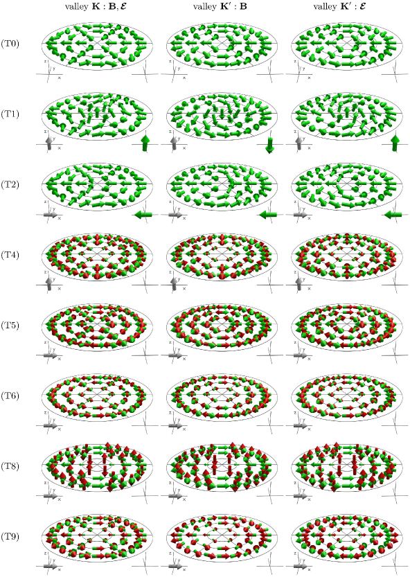
Figure 2: Visualization of real and pseudospin textures in BLG generated by field-dependent interactions shown in Table 3 [omitting the trivial interactions (T3) and (T7)]. The first row denoted (T0) shows the pseudospin texture without any external fields. For selected points in ${\bm{\mathrm{k}}}$ space, a red (green) arrow indicates the expectation value of the real (pseudo-)spin vector of the corresponding negative-energy eigenstate obtained by diagonalizing the leading field-independent contribution to the BLG Hamiltonian together with the respective term in Table 3. The 1st (2nd, 3rd) column shows results for the valley ${\bm{\mathrm{K}}}$ (${\bm{\mathrm{K^{\prime}}}}$ with ${\bm{\mathrm{B}}}$, ${\bm{\mathrm{K^{\prime}}}}$ with ${\bm{\mathcal{E}}}$). Note that our sign convention is such that ${\bm{\mathrm{B}}}$ and ${\bm{\mathcal{E}}}$ have the same effect in the ${\bm{\mathrm{K}}}$ valley (1st column). Gray arrows indicate the direction of the applied field. Big arrows in the lower right of the panels indicate the existence of a net spin polarization obtained by averaging over the (pseudo-)spin expectation values of occupied hole states for a negative chemical potential.

Similar to term (T3), according to term (T7), an in-plane magnetic field ${\bm{\mathrm{B}}}_{\|}$ gives rise to a macroscopic in-plane polarization of real spins whereas the real-spin polarization induced by an electric field ${\bm{\mathcal{E}}}_{\|}$ is anti-parallel in the two valleys. Fields ${\bm{\mathrm{B}}}_{\|}$ and ${\bm{\mathcal{E}}}_{\|}$ also couple to the in-plane pseudospin $\sigma_{\|}$. Term (T2) of Table 3 induces an out-of-plane tilt of the spin orientation of individual states which, in the ${\bm{\mathrm{K}}}^{\prime}$ valley, has opposite signs for ${\bm{\mathrm{B}}}_{\|}$ and ${\bm{\mathcal{E}}}_{\|}$. Remarkably, on average this yields an in-plane polarization $\langle{{\bm{\mathrm{\sigma}}}_{\|}}\rangle$ which is nonetheless the same in each valley for fields ${\bm{\mathrm{B}}}_{\|}$ and ${\bm{\mathcal{E}}}_{\|}$ (Fig. 2), see Appendix A.2 for a more quantitative discussion. This result reflects the fact that the macroscopic pseudospin polarization $\langle{{\bm{\mathrm{\sigma}}}_{\|}}\rangle$ is neither even nor odd under time reversal Winkler and Zülicke (2010). More precisely, in each valley the direction of $\langle{{\bm{\mathrm{\sigma}}}_{\|}}\rangle$ is well-defined only up to a gauge-dependent angular offset. Yet the change of $\langle{{\bm{\mathrm{\sigma}}}_{\|}}\rangle$ induced by a change in the in-plane orientation of the applied field is well-defined and it points clockwise in one valley and counterclockwise in the other valley (for both ${\bm{\mathrm{B}}}_{\|}$ and ${\bm{\mathcal{E}}}_{\|}$ and all terms in Tab. 3 giving rise to an in-plane pseudospin orientation of individual states). Specifically for the term (T2), if we change the in-plane orientation of the fields ${\bm{\mathrm{B}}}_{\|}$ or ${\bm{\mathcal{E}}}_{\|}$ by an angle $\varphi$, this changes the resulting average polarization $\langle{{\bm{\mathrm{\sigma}}}_{\|}}\rangle$ by $\pm 2\varphi$. This implies, in particular, that reverting the direction of the external field yields the same orientation of the induced pseudospin polarization (see Appendix A.2). We see here that the pseudospin polarization induced by external fields ${\bm{\mathcal{E}}}$ and ${\bm{\mathrm{B}}}$ behaves qualitatively different from the polarization of real spins. We emphasize that the measurable thermodynamic response due to the term (T2) (see previous subsection) is not affected by these ambiguities concerning the field-induced pseudospin textures.

The real spins also respond to electric and magnetic fields in unusual ways. Normally, a Zeeman term orients the spins parallel (or antiparallel) to the applied magnetic field. According to terms (T4), (T5), and (T6) a perpendicular magnetic field $B_{z}$ orients the spins in-plane and according to term (T8), an in-plane magnetic field can orient the spins out-of-plane. The Zeeman terms (T4), (T5), (T6), (T8) and (T9) orient the individual spins, but on average these terms do not give rise to a spin polarization (not even in individual valleys). Thus we have here no simple relation between the spin polarization and the thermodynamic magnetization. This is due to the fact that ultimately these terms are caused by spin-orbit coupling so that spin and orbital contributions to the magnetization (and dielectric polarization) cannot be discussed separately.

V Invariant Expansion for the SWM model of BLG

A unified picture of the magnitude of the various effects discussed above can be derived from the multiband SWM model of BLG. Indeed, the SWM model takes a similar role for BLG as the well-known multiband Kane model Kane (1966); Winkler (2003) for many zinc blende semiconductors, where Löwdin partitioning Löwdin (1951) can be used to predict the magnitude of effects like Zeeman splitting and Rashba spin-orbit coupling.

The theory of invariants (Sec. III) readily reproduces the ${\bm{\mathrm{k}}}$-dependent terms in the SWM Hamiltonian (13). An external field $\mathcal{E}_{z}$ results in the spin-independent and ${\bm{\mathrm{k}}}$-independent terms

$$\mathcal{H}^{\bm{\mathrm{K}}}_{\mathcal{E}}=\left(\begin{array}[]{s{0.15em}ccccs{0.15em}}\hskip 1.49994pt\lx@intercol\hfil 0&\varepsilon_{12}\mathcal{E}_{z}&0&0\hfil\hskip 1.49994pt\\ \hskip 1.49994pt\lx@intercol\hfil\varepsilon_{12}\mathcal{E}_{z}&0&0&0\hfil\hskip 1.49994pt\\ \hskip 1.49994pt\lx@intercol\hfil 0&0&\varepsilon_{33}\mathcal{E}_{z}&0\hfil\hskip 1.49994pt\\ \hskip 1.49994pt\lx@intercol\hfil 0&0&0&-\varepsilon_{33}\mathcal{E}_{z}\hfil\hskip 1.49994pt\end{array}\right).$$ (30)

Recent experiments Zhang et al. (2009) have demonstrated that a displacement field of $\sim 1$ V/nm generates a band gap of $\sim 0.1$ eV in BLG, corresponding to $\varepsilon_{33}\sim 0.05~{}e\,\mathrm{nm}$ or [see Eq. (2)]

$$g_{\mathrm{e}}=\frac{2\,c\,\varepsilon_{33}}{\mu_{B}}\simeq 500\quad.$$ (31)

This value is reasonably close to the expected potential difference induced by a field $\mathcal{E}_{z}$ between the $B$ and $B^{\prime}$ layer of BLG with an inter-layer separation $0.34$ nm that gets effectively reduced by screening. We may expect a similar potential difference induced between the layers $A$ and $A^{\prime}$, implying $\varepsilon_{12}\simeq\varepsilon_{33}$. This is also consistent with the ab-initio calculations in Ref. Konschuh et al., 2012 that found $\varepsilon_{12}=\varepsilon_{33}=0.048~{}e\,\mathrm{nm}$.

It follows from Tables 1 and 2 and Eq. (20) that intrinsic (Pauli) spin-orbit coupling results in the terms

$$\mathcal{H}^{\bm{\mathrm{K}}}_{p}=\left(\begin{array}[]{s{0.15em}ccccs{0.15em}}\hskip 1.49994pt\lx@intercol\hfil 0&p_{12}s_{z}&2ip_{13}s_{-}&2ip_{13}s_{+}\hfil\hskip 1.49994pt\\ \hskip 1.49994pt\lx@intercol\hfil p_{12}s_{z}&0&2ip_{23}s_{-}&-2ip_{23}s_{+}\hfil\hskip 1.49994pt\\ \hskip 1.49994pt\lx@intercol\hfil-2ip_{13}s_{+}&-2ip_{23}s_{+}&p_{33}s_{z}&0\hfil\hskip 1.49994pt\\ \hskip 1.49994pt\lx@intercol\hfil-2ip_{13}s_{-}&2ip_{23}s_{-}&0&-p_{33}s_{z}\hfil\hskip 1.49994pt\end{array}\right).$$ (32)

Rashba spin-orbit coupling results in the terms

$$\mathcal{H}^{\bm{\mathrm{K}}}_{r}=\mathcal{E}_{z}\left(\begin{array}[]{s{0.15em}ccccs{0.15em}}\hskip 1.49994pt\lx@intercol\hfil r_{11}s_{z}&0&2ir_{13}s_{-}&-2ir_{13}s_{+}\hfil\hskip 1.49994pt\\ \hskip 1.49994pt\lx@intercol\hfil 0&r_{22}s_{z}&2ir_{23}s_{-}&2ir_{23}s_{+}\hfil\hskip 1.49994pt\\ \hskip 1.49994pt\lx@intercol\hfil-2ir_{13}s_{+}&-2ir_{23}s_{+}&r_{33}^{\prime}s_{z}&ir_{33}s_{-}\hfil\hskip 1.49994pt\\ \hskip 1.49994pt\lx@intercol\hfil 2ir_{13}s_{-}&-2ir_{23}s_{-}&-ir_{33}s_{+}&r_{33}^{\prime}s_{z}\hfil\hskip 1.49994pt\end{array}\right).$$ (33)

Here we have used the phase convention that all prefactors are real.

The magnitude of spin-orbit coupling in BLG was recently studied by Konschuh et al. (Ref. Konschuh et al., 2012), who developed a generalized SWM-like tight-binding model that they fitted to the results of numerical ab-initio calculations. To compare their work with ours, we need to apply the unitary transformation $U^{-1}HU$ to Eqs. (2) and (8) of Ref. Konschuh et al., 2012 with

$$U=\left(\begin{array}[]{s{0.15em}ccccs{0.15em}}\hskip 1.49994pt\lx@intercol\hfil\frac{1}{\sqrt{2}}&\frac{1}{\sqrt{2}}&0&0\hfil\hskip 1.49994pt\\[4.30554pt] \hskip 1.49994pt\lx@intercol\hfil 0&0&-1&0\hfil\hskip 1.49994pt\\[4.30554pt] \hskip 1.49994pt\lx@intercol\hfil 0&0&0&-1\hfil\hskip 1.49994pt\\[4.30554pt] \hskip 1.49994pt\lx@intercol\hfil\frac{1}{\sqrt{2}}&-\frac{1}{\sqrt{2}}&0&0\hfil\hskip 1.49994pt\end{array}\right).$$ (34)

The orbital TB Hamiltonian (2) in Ref. Konschuh et al., 2012 is then identical in form to our Eq. (11), except for the terms proportional to $\gamma_{4}$ which have the opposite sign. The unitary transformation of the SO Hamiltonian (8) in Ref. Konschuh et al., 2012 yields

$$\begin{array}[b]{rl}U^{-1}H_{\mathrm{SO}}U=&\left(\begin{array}[]{s{0.15em}*{4}{>{\Ds}c}s{0.15em}}\hskip 1.49994pt\lx@intercol\hfil\displaystyle\frac{\lambda_{\mathrm{I}2}-\lambda_{\mathrm{I}2}^{\prime}}{2}s_{z}&\displaystyle\frac{\lambda_{\mathrm{I}2}+\lambda_{\mathrm{I}2}^{\prime}}{2}s_{z}&\displaystyle-i\frac{\bar{\lambda}_{0}+\bar{\lambda}_{4}}{\sqrt{2}}s_{-}&\displaystyle-i\frac{\bar{\lambda}_{0}+\bar{\lambda}_{4}}{\sqrt{2}}s_{+}\hfil\hskip 1.49994pt\\ \hskip 1.49994pt\lx@intercol\hfil\displaystyle\frac{\lambda_{\mathrm{I}2}+\lambda_{\mathrm{I}2}^{\prime}}{2}s_{z}&\displaystyle\frac{\lambda_{\mathrm{I}2}-\lambda_{\mathrm{I}2}^{\prime}}{2}s_{z}&\displaystyle-i\frac{\bar{\lambda}_{0}-\bar{\lambda}_{4}}{\sqrt{2}}s_{-}&\displaystyle i\frac{\bar{\lambda}_{0}-\bar{\lambda}_{4}}{\sqrt{2}}s_{+}\hfil\hskip 1.49994pt\\ \hskip 1.49994pt\lx@intercol\hfil\displaystyle i\frac{\bar{\lambda}_{0}+\bar{\lambda}_{4}}{\sqrt{2}}s_{+}&\displaystyle i\frac{\bar{\lambda}_{0}-\bar{\lambda}_{4}}{\sqrt{2}}s_{+}&\displaystyle-\lambda_{\mathrm{I}1}s_{z}&\displaystyle 0\hfil\hskip 1.49994pt\\ \hskip 1.49994pt\lx@intercol\hfil\displaystyle i\frac{\bar{\lambda}_{0}+\bar{\lambda}_{4}}{\sqrt{2}}s_{-}&\displaystyle-i\frac{\bar{\lambda}_{0}-\bar{\lambda}_{4}}{\sqrt{2}}s_{-}&\displaystyle 0&\displaystyle\lambda_{\mathrm{I}1}^{\prime}s_{z}\hfil\hskip 1.49994pt\end{array}\right)\\ \\ +&\left(\begin{array}[]{s{0.15em}*{4}{>{\Ds}c}s{0.15em}}\hskip 1.49994pt\lx@intercol\hfil\displaystyle\lambda_{1}s_{z}&\displaystyle 0&\displaystyle-i\frac{2\lambda_{\mathrm{BR}}-\delta\lambda_{4}}{\sqrt{2}}s_{-}&\displaystyle i\frac{2\lambda_{\mathrm{BR}}-\delta\lambda_{4}}{\sqrt{2}}s_{+}\hfil\hskip 1.49994pt\\ \hskip 1.49994pt\lx@intercol\hfil\displaystyle 0&\displaystyle-\lambda_{1}s_{z}&\displaystyle-i\frac{2\lambda_{\mathrm{BR}}+\delta\lambda_{4}}{\sqrt{2}}s_{-}&\displaystyle-i\frac{2\lambda_{\mathrm{BR}}+\delta\lambda_{4}}{\sqrt{2}}s_{+}\hfil\hskip 1.49994pt\\ \hskip 1.49994pt\lx@intercol\hfil\displaystyle i\frac{2\lambda_{\mathrm{BR}}-\delta\lambda_{4}}{\sqrt{2}}s_{+}&\displaystyle i\frac{2\lambda_{\mathrm{BR}}+\delta\lambda_{4}}{\sqrt{2}}s_{+}&\displaystyle 0&\displaystyle i\lambda_{3}s_{-}\hfil\hskip 1.49994pt\\ \hskip 1.49994pt\lx@intercol\hfil\displaystyle-i\frac{2\lambda_{\mathrm{BR}}-\delta\lambda_{4}}{\sqrt{2}}s_{-}&\displaystyle i\frac{2\lambda_{\mathrm{BR}}+\delta\lambda_{4}}{\sqrt{2}}s_{-}&\displaystyle-i\lambda_{3}s_{+}&\displaystyle 0\hfil\hskip 1.49994pt\end{array}\right),\end{array}$$ (35)

where the first matrix describes the intrinsic SO coupling and the second matrix gives the SO coupling induced by an external electric field $\mathcal{E}_{z}$. Comparing with Eq. (32), we thus get the correspondence

$$p_{12} = {\textstyle\frac{1}{2}}(\lambda_{\mathrm{I}2}+\lambda_{\mathrm{I}2}^{\prime}),$$ (36a)

$$p_{13} = -(\bar{\lambda}_{0}+\bar{\lambda}_{4})/\sqrt{8},$$ (36b)

$$p_{23} = -(\bar{\lambda}_{0}-\bar{\lambda}_{4})/\sqrt{8},$$ (36c)

$$p_{33} = -(\lambda_{\mathrm{I}1}+\lambda_{\mathrm{I}1}^{\prime})/2.$$ (36d)

By symmetry, we must have $\lambda_{\mathrm{I}1}=\lambda_{\mathrm{I}1}^{\prime}$ and $\lambda_{\mathrm{I}2}=\lambda_{\mathrm{I}2}^{\prime}$. For the SO terms induced by an electric field $\mathcal{E}_{z}$ [Eq. (33)] we get the correspondence

$$r_{11}\,\mathcal{E}_{z} = -r_{22}\,\mathcal{E}_{z}=\lambda_{1},$$ (37a)

$$r_{13}\,\mathcal{E}_{z} = -(\lambda_{\mathrm{BR}}-\delta\lambda_{4}/2)/\sqrt{2},$$ (37b)

$$r_{23}\,\mathcal{E}_{z} = -(\lambda_{\mathrm{BR}}+\delta\lambda_{4}/2)/\sqrt{2},$$ (37c)

$$r_{33}\,\mathcal{E}_{z} = \lambda_{3}.$$ (37d)

The term proportional to $r_{33}^{\prime}$ is absent in Ref. Konschuh et al., 2012.

A least-square fit of the numerical ab-initio results in Ref. Konschuh et al., 2012 to the intrinsic SO Hamiltonian (32) indicates (consistent with the findings in Ref. Konschuh et al., 2012) that all four coefficients $p_{ij}$ contribute significantly to the intrinsic SO coupling

$$p_{12} =10.8~{}\mathrm{\mu eV}, p_{33} =-12.1~{}\mathrm{\mu eV},$$ (38a)

$$p_{13} =4.3~{}\mathrm{\mu eV}, p_{23} =-4.8~{}\mathrm{\mu eV}.$$ (38b)

On the other hand, we find that Rashba SO coupling in the $4\times 4$ SWM model [Eq. (33)] is dominated by the coefficients

$$r_{13}=-5.0~{}e\,\mathrm{fm}\;,\hskip 30.00005ptr_{23}=-1.6~{}e\,\mathrm{fm}\quad.$$ (39)

The coefficients $r_{11}$, $r_{22}$, $r_{33}$, and $r_{33}^{\prime}$ in the diagonal blocks are found to contribute only marginally to Rashba SO coupling according to a comparison with the ab-initio results in Ref. Konschuh et al., 2012.

VI Löwdin partitioning for the SWM model of BLG

Löwdin partitioning Bir and Pikus (1974); Winkler (2003) can provide explicit expressions for the prefactors of many terms discussed in this work. Here the starting point is the $4\times 4$ SWM Hamiltonian (13) complemented by the field term (30), the Pauli Hamiltonian (32), the Rashba SO Hamiltonian (33) as well as the potential due to an external electric field ${\bm{\mathcal{E}}}$;

$$\mathcal{H}^{\bm{\mathrm{K}}}=\mathcal{H}^{\bm{\mathrm{K}}}_{\bm{\mathrm{k}}}+\mathcal{H}^{\bm{\mathrm{K}}}_{\mathcal{E}}+\mathcal{H}^{\bm{\mathrm{K}}}_{p}+\mathcal{H}^{\bm{\mathrm{K}}}_{r}+{\bm{\mathcal{E}}}\cdot{\bm{\mathrm{r}}}\;.$$ (40)

The $4\times 4$ model $\mathcal{H}^{\bm{\mathrm{K}}}$ provides a comprehensive description of the electron dynamics in BLG in the presence of electric and magnetic fields as well as intrinsic and extrinsic SO coupling. Zeeman-like terms proportional to $B_{z}$ arise in Löwdin partitioning due to the noncommutativity of the components of kinetic crystal momentum $\hbar{\bm{\mathrm{k}}}$, where $[k_{x},k_{y}]=(e/i\hbar)B_{z}$. Similarly, Rashba-like terms proportional to an in-plane electric field ${\bm{\mathcal{E}}}_{\|}=(\mathcal{E}_{x},\mathcal{E}_{y},0)$ arise from the commutator between the last term in Eq. (40) and the operator ${\bm{\mathrm{k}}}$ Winkler (2003); abi .

As noted in the previous section, a least-square fit to the ab-initio calculations in Ref. Konschuh et al., 2012 cannot provide reliable values for the prefactors $r_{11}$, $r_{22}$, $r_{33}$, and $r_{33}^{\prime}$ in $\mathcal{H}^{\bm{\mathrm{K}}}_{r}$. However, if we project the $4\times 4$ Hamiltonian (40) on the subspaces $(\mathcal{H}^{\bm{\mathrm{K}}})_{11}$, $(\mathcal{H}^{\bm{\mathrm{K}}})_{22}$, and $(\mathcal{H}^{\bm{\mathrm{K}}})_{33}$, we obtain in lowest order

$$\tilde{r}_{11} = \frac{\varepsilon_{12}\,p_{12}}{\gamma_{1}}-\frac{8p_{13}\,r_{13}}{\gamma_{1}},$$ (41a)

$$\tilde{r}_{22} = -\frac{\varepsilon_{12}\,p_{12}}{\gamma_{1}}+\frac{8p_{23}\,r_{23}}{\gamma_{1}},$$ (41b)

$$\tilde{r}_{33} = 0,\hskip 20.00003pt\tilde{r}_{33}^{\prime}=\frac{4(p_{23}\,r_{23}-p_{13}\,r_{13})}{\gamma_{1}}$$ (41c)

where the tilde indicates that these expressions are valid only within the respective projected subspaces. These formulas indicate that the $k$-independent Rashba spin splitting in the subspaces $(\mathcal{H}^{\bm{\mathrm{K}}})_{11}$ and $(\mathcal{H}^{\bm{\mathrm{K}}})_{22}$ is of first order in SO coupling whereas it is of second order in the $(\mathcal{H}^{\bm{\mathrm{K}}})_{33}$ subspace, consistent with the numerical ab-initio calculations in Ref. Konschuh et al., 2012.

Most often we are interested only in the subspace $(\mathcal{H}^{\bm{\mathrm{K}}})_{33}$. In Table 4 we summarize the most important terms appearing in the Löwdin projection of $\mathcal{H}^{\bm{\mathrm{K}}}$ onto the subspace $(\mathcal{H}^{\bm{\mathrm{K}}})_{33}$.

Table 4: Prefactors of selected terms in $\mathcal{H}_{33}$, obtained via Löwdin partitioning of the SWM model. Both the expressions in terms of SWM parameters as well as the numerical values are given. The place in this article where a term has been introduced is also referenced. In the first column, the upper sign holds for valley ${\bm{\mathrm{K}}}$, the lower sign for ${\bm{\mathrm{K}}}^{\prime}$.

term	prefactor (parametric)	prefactor (numeric)	introduced in
$-(k_{-}\,\sigma_{\pm}+k_{+}\,\sigma_{\mp})\,\tau_{z}$	$\displaystyle\tilde{\gamma}_{31}$	$0.053~{}\mathrm{eV^{2}\,nm}$	(1)
$k^{2}\,\tau_{0}$	$\displaystyle\tilde{\gamma}_{0}^{\prime}+\frac{2\tilde{\gamma}_{0}\tilde{\gamma}_{4}}{\gamma_{1}}$	$0.13~{}\mathrm{eV\,nm^{2}}$	(1)
$-(k_{+}^{2}\,\sigma_{\pm}+k_{-}^{2}\,\sigma_{\mp})\,\tau_{0}$	$\displaystyle-\tilde{\gamma}_{32}+\frac{\tilde{\gamma}_{0}^{2}+\tilde{\gamma}_{4}^{2}}{\gamma_{1}}$	$1.3~{}\mathrm{eV\,nm^{2}}$	(1)
$s_{z}\sigma_{z}\tau_{z}$	$\displaystyle p_{33}$	$-12~{}\mathrm{\mu eV}$	(42a)
$i(s_{+}k_{-}-s_{-}k_{+})\sigma_{z}\,\tau_{z}$	$\displaystyle\frac{\sqrt{2}\,[\tilde{\gamma}_{0}(p_{13}-p_{23})-\tilde{\gamma}_{4}(p_{13}+p_{23})]}{\gamma_{1}}$	$18~{}\mathrm{\mu eV\,nm}$	(42b)
$\rule{0.0pt}{17.22217pt}B_{z}\sigma_{z}\,\tau_{z}$	$\displaystyle-\frac{2\tilde{\gamma}_{0}\tilde{\gamma}_{4}}{\gamma_{1}}\frac{e}{\hbar}$	$-180~{}\mathrm{\mu eV/T}$	(T1)
$\mathcal{E}_{z}\sigma_{z}\,\tau_{0}$	$\displaystyle\varepsilon_{33}$	$0.048~{}e\,\mathrm{nm}$	(T1)
$\mathcal{E}_{z}B_{z}\,\tau_{z}$	$\displaystyle\frac{\tilde{\gamma}_{0}^{2}(\varepsilon_{33}+\varepsilon_{12})+\tilde{\gamma}_{4}^{2}(\varepsilon_{33}-\varepsilon_{12})}{\gamma_{1}^{2}}\,\frac{e}{\hbar}$	$5.8\times 10^{-4}~{}e\,\mathrm{nm/T}$	(2)
$\rule{0.0pt}{19.37494pt}(i/2)(k_{+}\mathcal{E}_{-}-k_{-}\mathcal{E}_{+})\sigma_{z}\,\tau_{z}$	$\displaystyle\frac{(\tilde{\gamma}_{0}^{2}+\tilde{\gamma}_{4}^{2})\,e}{\gamma_{1}^{2}}$	$4.0~{}e\,\mathrm{nm^{2}}$	(T2)
$\rule{0.0pt}{19.37494pt}B_{z}s_{z}\,\tau_{0}$	$\displaystyle\frac{\tilde{\gamma}_{0}^{2}(p_{33}+p_{12})+\tilde{\gamma}_{4}^{2}(p_{33}-p_{12})}{\gamma_{1}^{2}}\frac{e}{\hbar}$	$-9.3\times 10^{-9}~{}\mathrm{eV/T}$	(T3)
$\mathcal{E}_{z}s_{z}\,\tau_{z}$	$\displaystyle r_{33}^{\prime}+\frac{4(p_{23}\,r_{23}-p_{13}\,r_{13})}{\gamma_{1}}$	$3.6\times 10^{-10}~{}e\,\mathrm{nm}$	(T3)
$\mathcal{E}_{z}B_{z}s_{z}\sigma_{z}\,\tau_{0}$	$\displaystyle\frac{r_{33}^{\prime}(\tilde{\gamma}_{0}^{2}+\tilde{\gamma}_{4}^{2})}{\gamma_{1}^{2}}\frac{e}{\hbar}$	$\approx 0$
$\rule{0.0pt}{19.37494pt}2iB_{z}(s_{-}\sigma_{\pm}-s_{+}\sigma_{\mp})\,\tau_{0}$	$\displaystyle-\frac{\tilde{\gamma}_{31}[\tilde{\gamma}_{0}(p_{23}+p_{13})+\tilde{\gamma}_{4}(p_{23}-p_{13})]}{\sqrt{2}\,\gamma_{1}^{2}}\frac{e}{\hbar}$	$3.3\times 10^{-10}~{}\mathrm{eV/T}$	(T4)
$2i\mathcal{E}_{z}(s_{-}\sigma_{\pm}-s_{+}\sigma_{\mp})\,\tau_{z}$	$\displaystyle r_{33}$	$\approx 0$	(T4)
$\rule{0.0pt}{19.37494pt}iB_{z}(s_{+}k_{-}-s_{-}k_{+})\,\tau_{z}$	$\displaystyle\frac{\sqrt{2}\,\tilde{\gamma}_{0}^{\prime}[\tilde{\gamma}_{0}(p_{23}+p_{13})+\tilde{\gamma}_{4}(p_{23}-p_{13})]}{\gamma_{1}^{2}}\frac{e}{\hbar}$	$1.6\times 10^{-7}~{}\mathrm{eV\,nm/T}$	(T5)
$i\mathcal{E}_{z}(s_{+}k_{-}-s_{-}k_{+})\,\tau_{0}$	$\displaystyle\frac{\sqrt{2}\,[\tilde{\gamma}_{0}(r_{13}-r_{23})-\tilde{\gamma}_{4}(r_{13}+r_{23})]}{\gamma_{1}}$	$8.7\times 10^{-6}~{}e\,\mathrm{nm^{2}}$	(T5)
$2iB_{z}(s_{-}k_{-}\sigma_{\mp}-s_{+}k_{+}\sigma_{\pm})\,\tau_{z}$	$\displaystyle\frac{\sqrt{2}}{\gamma_{1}^{2}}\begin{array}[t]{@{}r@{}l@{}}\{&\tilde{\gamma}_{0}^{\prime}[\tilde{\gamma}_{0}(p_{13}-p_{23})-\tilde{\gamma}_{4}(p_{13}+p_{23})]\\ \makebox[0.0pt][r]{${}+{}$}&\tilde{\gamma}_{32}[\tilde{\gamma}_{4}(p_{13}-p_{23})-\tilde{\gamma}_{0}(p_{13}+p_{23})]\}\displaystyle\frac{e}{\hbar}\end{array}$	$-2.9\times 10^{-8}~{}\mathrm{eV\,nm/T}$	(T6)
$2i\mathcal{E}_{z}(s_{-}k_{-}\sigma_{\mp}-s_{+}k_{+}\sigma_{\pm})\,\tau_{0}$	$\displaystyle\frac{\sqrt{2}\,[\tilde{\gamma}_{4}(r_{13}-r_{23})-\tilde{\gamma}_{0}(r_{13}+r_{23})]}{\gamma_{1}}$	$2.2\times 10^{-5}~{}e\,\mathrm{nm^{2}}$	(T6)
$\rule{0.0pt}{19.37494pt}(\mathcal{E}_{+}s_{-}+\mathcal{E}_{-}s_{+})\,\tau_{z}$	$\displaystyle\frac{[\tilde{\gamma}_{0}(p_{23}+p_{13})+\tilde{\gamma}_{4}(p_{23}-p_{13})]\,e}{\sqrt{2}\,\gamma_{1}^{2}}$	$-4.1\times 10^{-6}~{}e\,\mathrm{nm}$	(T7)
$i(\mathcal{E}_{-}\sigma_{\pm}-\mathcal{E}_{+}\sigma_{\mp})s_{z}\,\tau_{z}$	$\displaystyle 0$	$0$	(T8)
$-2(\mathcal{E}_{+}s_{+}\sigma_{\pm}+\mathcal{E}_{-}s_{-}\sigma_{\mp})\,\tau_{z}$	$\displaystyle\frac{[\tilde{\gamma}_{0}(p_{23}-p_{13})+\tilde{\gamma}_{4}(p_{23}+p_{13})]\,e}{\sqrt{2}\,\gamma_{1}^{2}}$	$-4.0\times 10^{-6}~{}e\,\mathrm{nm}$	(T9)

Intrinsic spin splitting in BLG is dominated by two terms, the $k$-independent term

$$s_{z}\sigma_{z}\,\tau_{z}$$ (42a)

orienting the spins out-of-plane as well as the $$k$$-linear term

$$i\left(s_{+}k_{-}-s_{-}k_{+}\right)\sigma_{z}\,\tau_{0}$$ (42b)

orienting the spins in-plane. For typical Fermi wave vectors these terms are similar in magnitude. The combined effect of both terms is a vortex-like spin texture in the $(k_{x},k_{y})$ plane around the ${\bm{\mathrm{K}}}$ point. Interestingly, we get rather similar spin textures from a magnetic field $B_{z}$ or an electric field $\mathcal{E}_{z}$ via the terms (T3), (T5) and (T6) though in each case the ratio between the respective prefactors is different.

It is helpful to express the prefactors of the magnetic terms (T1), (T3), and (T4) in terms of effective $g$ factors, giving the numeric values $6.2$, $3.2\times 10^{-4}$, and $1.1\times 10^{-5}$, respectively. The latter two values represent actually the correction to the $g$ factor $g=2$ of free electrons, similar to the well-known Roth formula Roth et al. (1959). Also, we may compare the magnitude of the couplings for the pairs of electric and magnetic terms in Table 3, noting that for an electric field $\mathcal{E}$ the term $\mathcal{E}/c$ has the same dimension tesla as a magnetic field $B$. For the term (T1), this yields $g_{\mathrm{e}}/g_{\mathrm{m}}\approx 80$, (T3) gives the ratio $\sim 0.012$, (T5) $\sim 16$ and (T6) $\sim 230$. The ratio of the couplings to the electric and magnetic fields is thus not universal.

VII Conclusions and Outlook

Our study of the electronic structure of BLG in the presence of electric and magnetic fields has revealed that this material exhibits an unusual magneto-electric equivalence: Every possible coupling of a spin or pseudospin component to the electric (magnetic) field is complemented by an analogous coupling to the magnetic (electric) field. Such a behavior, while counter-intuitive, is consistent with basic requirements arising from spatial and time-reversal symmetries. It implies that the thermodynamic response to a magnetic field (the magnetization) takes the same functional form as the response to an electric field (the polarization). Based on Löwdin partitioning for the multiband SWM model of the BLG band structure and using input from ab-initio and tight-binding calculations, we have obtained numerical prefactors for relevant coupling terms.

Our work has focused on BLG, for which the well-established SWM model provides a convenient basis for a systematic discussion. However, we would like to emphasize that the group-theoretical arguments used here are valid more generally for any multi-valley material with similar symmetries such as silicene Geissler et al. (2013) and asymmetrically hydrogenated single-layer graphene Gmitra et al. (2013). The recent interest in topological insulators has also stimulated a quest for novel layered materials with strong spin-orbit coupling such as Bi₂Se₃ and Sb₂Te₃, where individual layers form a hexagonal structure similar to BLG Yan and Zhang (2012) and therefore can be expected to have similar electrodynamic properties.

Besides shedding new light on emergent electromagnetism in unconventional materials, our discussion of unusual couplings between electric and magnetic fields to spins and pseudospins due to magneto-electric equivalence also opens up new possibilities for creating spintronic and valleytronic devices.

Appendix A Pseudospin Polarization

In this appendix, we study more quantitatively the pseudospin polarization induced by external fields ${\bm{\mathcal{E}}}$ and ${\bm{\mathrm{B}}}$. In the following we denote these fields by the generic placeholder ${\bm{\mathcal{F}}}$.

A.1 BLG in perpendicular fields ${\bm{\mathcal{F}}}_{z}$

We consider the BLG Hamiltonian with term (T1) from Table 3, using the simplified notation

$$\mathcal{H}=a\left(k_{+}^{2}\,\sigma_{+}+k_{-}^{2}\,\sigma_{-}\right)+c_{f,z}\mathcal{F}_{z}\sigma_{z}\;.$$ (43)

Writing the wave vector in polar coordinates ${\bm{\mathrm{k}}}=(k,\phi)$, the Hamiltonian becomes

$$\mathcal{H}=ak^{2}\left(\begin{array}[]{s{0.15em}ccs{0.15em}}\hskip 1.49994pt\lx@intercol\hfil b_{z}&-e^{2i\phi}\hfil\hskip 1.49994pt\\[4.30554pt] \hskip 1.49994pt\lx@intercol\hfil-e^{-2i\phi}&-b_{z}\hfil\hskip 1.49994pt\end{array}\right)\;,$$ (44)

with $b_{z}\equiv c_{f,z}\mathcal{F}_{z}/(ak^{2})$. The pseudospin orientation of the eigenstates $|{{\bm{\mathrm{k}}}}\rangle_{\pm}$ is $\langle{{\bm{\mathrm{\sigma}}}}\rangle({\bm{\mathrm{k}}},\pm)\equiv\langle{{\bm{\mathrm{k}}}|{\bm{\mathrm{\sigma}}}|{\bm{\mathrm{k}}}}\rangle_{\pm}$, giving

$$\langle{\sigma_{x}}\rangle({\bm{\mathrm{k}}},\pm) = \mp\frac{\cos(2\phi)}{\sqrt{1+b_{z}^{2}}}\;,$$ (45a)

$$\langle{\sigma_{y}}\rangle({\bm{\mathrm{k}}},\pm) = \pm\frac{\sin(2\phi)}{\sqrt{1+b_{z}^{2}}}\;,$$ (45b)

$$\langle{\sigma_{z}}\rangle({\bm{\mathrm{k}}},\pm) = \pm\frac{b}{\sqrt{1+b_{z}^{2}}}\;.$$ (45c)

The average pseudospin polarization at $T=0$ becomes

$$\langle{{\bm{\mathrm{\sigma}}}}\rangle_{\pm}=\frac{2}{k_{\mathrm{F}}^{2}}\int_{0}^{k_{\mathrm{F}}}dk\,k\int_{0}^{2\pi}\frac{d\phi}{2\pi}\;\langle{{\bm{\mathrm{k}}}|{\bm{\mathrm{\sigma}}}|{\bm{\mathrm{k}}}}\rangle_{\pm}\;,$$ (46)

giving

$$\langle{\sigma_{x}}\rangle_{\pm} = \langle{\sigma_{y}}\rangle_{\pm}=0\;,$$ (47a)

$$\langle{\sigma_{z}}\rangle_{\pm} = \pm b_{\mathrm{F},z}\,\ln\frac{1+\sqrt{1+b_{\mathrm{F},z}^{2}}}{b_{\mathrm{F},z}}\;,$$ (47b)

with $b_{\mathrm{F},z}\equiv c_{f,z}\mathcal{F}_{z}/(ak_{\mathrm{F}}^{2})$. We can express the average polarization $\langle{\sigma_{z}}\rangle_{\pm}$ in terms of the Fermi energy $E_{\mathrm{F}}=ak_{\mathrm{F}}^{2}\,\sqrt{1+b_{\mathrm{F},z}^{2}}$ as

$$\langle{\sigma_{z}}\rangle_{\pm}=\pm\frac{\tilde{b}_{z}}{\sqrt{1-\tilde{b}_{z}^{2}}}\,\ln\frac{1+\sqrt{1-\tilde{b}_{z}^{2}}}{\tilde{b}_{z}}\quad,$$ (48)

with $\tilde{b}_{z}=c_{f,z}\mathcal{F}_{z}/E_{\mathrm{F}}$. As to be expected, we only have a nonzero $z$ component of the pseudospin polarization, which changes sign when the sign of $b$ is changed. We emphasize that the above formulas are valid for both magnetic and electric fields, which illustrates nicely the concept of magneto-electric equivalence.

We have $a=\hbar^{2}u/(2m_{0})\approx 1.27$ eV nm² and a typical density is $n\simeq 2.5\times 10^{12}$ cm^-2 (Ref. Novoselov et al., 2006) giving $k_{\mathrm{F}}=\sqrt{\pi\,n}\simeq 0.28$ nm^-1 and $ak_{\mathrm{F}}^{2}\simeq 0.1$ eV. For the electric term, we have $g_{\mathrm{e}}\approx 500$ or $c_{\mathrm{e},z}=g_{\mathrm{e}}\,\mu_{\mathrm{B}}/(2c)=\varepsilon_{33}\approx 0.05~{}e\,\mathrm{nm}$, so that $\mathcal{E}_{z}\sim 1$ V/nm corresponds to an electric energy $c_{\mathrm{e},z}\mathcal{E}_{z}\approx 50$ meV, giving $b_{\mathrm{e,F},z}\sim 0.5$ and $\langle{\sigma_{z}}\rangle_{\pm}=\pm 0.76$. For the corresponding magnetic term, we have $g_{\mathrm{m}}\approx 6.2$ or $c_{\mathrm{m},z}=g_{\mathrm{m}}\,\mu_{\mathrm{B}}/2\approx 0.18$ meV/T, so that a magnetic field $B_{z}=10$ T corresponds to a magnetic energy $c_{\mathrm{m},z}B_{z}=1.8$ meV giving $b_{\mathrm{m,F},z}\sim 0.018$ and $\langle{\sigma_{z}}\rangle_{\pm}=\pm 0.085$.

A.2 BLG in parallel fields ${\bm{\mathcal{F}}}_{\|}$

Next we consider the BLG Hamiltonian with term (T2) from Table 3,

$$\mathcal{H}=a\left(k_{+}^{2}\,\sigma_{+}+k_{-}^{2}\,\sigma_{-}\right)+c_{f\|}\,(k_{x}\mathcal{F}_{y}-k_{y}\mathcal{F}_{x})\sigma_{z}\;.$$ (49)

We use polar coordinates ${\bm{\mathcal{F}}}_{\|}=(\mathcal{F},\theta)$ giving

$$\mathcal{H}=ak^{2}\left(\begin{array}[]{s{0.15em}ccs{0.15em}}\hskip 1.49994pt\lx@intercol\hfil-\sqrt{2}\,b_{\|}/k&-e^{2i\phi}\hfil\hskip 1.49994pt\\[4.30554pt] \hskip 1.49994pt\lx@intercol\hfil-e^{-2i\phi}&\sqrt{2}\,b_{\|}/k\hfil\hskip 1.49994pt\end{array}\right)\;,$$ (50)

with $b_{\|}=(c_{f\|}\mathcal{F}/\sqrt{2}a)\,\sin(\phi-\theta)$. We can then immediately express the pseudospin orientation $\langle{{\bm{\mathrm{\sigma}}}}\rangle({\bm{\mathrm{k}}},\pm)$ of individual states similar to Eq. (45). To obtain the average pseudospin polarization of all occupied states up to the Fermi energy $E_{F}$, we switch from an integration over $k$ to an integration over energy $E$ using

$$k=\sqrt{\sqrt{E^{2}/a^{2}+b_{\|}^{4}}-b_{\|}^{2}}\quad.$$ (51)

The pseudospin orientation of individual states becomes then

$$\langle{\sigma_{x}}\rangle({\bm{\mathrm{k}}},\pm) = \mp\frac{\sqrt{E^{2}+a^{2}b_{\|}^{4}}-ab_{\|}^{2}}{E}\,\cos(2\phi)\;,$$ (52a)

$$\langle{\sigma_{y}}\rangle({\bm{\mathrm{k}}},\pm) = \pm\frac{\sqrt{E^{2}+a^{2}b_{\|}^{4}}-ab_{\|}^{2}}{E}\,\sin(2\phi)\;,\hskip 20.00003pt$$ (52b)

$$\langle{\sigma_{z}}\rangle({\bm{\mathrm{k}}},\pm) = \mp\frac{\sqrt{2}b_{\|}\,\sqrt{\sqrt{E^{2}+a^{2}b_{\|}^{4}}-ab_{\|}^{2}}}{E}\;.$$ (52c)

Using the fact that

$$\int d^{2}k\equiv\int d\phi\int dk\,k=\frac{1}{2a}\int d\phi\int dE\,\frac{E}{\sqrt{E^{2}+a^{2}b_{\|}^{4}}}\,\,,$$ (53)

and applying the proper normalization condition, we find

$$\langle{\sigma_{x}}\rangle_{\pm} = \mp\mathcal{P}(\tilde{b}_{\|})\,\cos(2\theta)\;,$$ (54a)

$$\langle{\sigma_{y}}\rangle_{\pm} = \pm\mathcal{P}(\tilde{b}_{\|})\,\sin(2\theta)\;,$$ (54b)

$$\langle{\sigma_{z}}\rangle_{\pm} = 0\;,$$ (54c)

with

$$\mathcal{P}(\tilde{b}_{\|})=\frac{\displaystyle\int_{0}^{2\pi}\!\!\!d\phi\,\cos(2\phi)\,\sin^{2}(\phi)\,\ln\left[\frac{\tilde{b}_{\|}+\sqrt{\tilde{b}_{\|}^{2}+\sin^{4}(\phi)}}{\sin^{2}(\phi)}\right]}{\displaystyle\pi-\int_{0}^{2\pi}\!\!d\phi\,\sqrt{\tilde{b}_{\|}^{2}+\sin^{4}(\phi)}}$$ (55)

and $\tilde{b}_{\|}\equiv 2aE_{\mathrm{F}}/(c_{f\|}^{2}\mathcal{F}^{2})$.

It follows from Eq. (54) that changing the orientation of ${\bm{\mathcal{F}}}_{\|}$ by the angle $\theta$ clockwise changes $\langle{{\bm{\mathrm{\sigma}}}}\rangle_{\pm}$ by $2\theta$ counterclockwise. We have, therefore, no simple geometric relation between the orientation of ${\bm{\mathcal{F}}}_{\|}$ and the orientation of the pseudospin polarization $\langle{{\bm{\mathrm{\sigma}}}}\rangle$. With our phase conventions in the ${\bm{\mathrm{K}}}$ valley electric and magnetic fields couple in the same way to the pseudospin whereas they couple oppositely in the ${\bm{\mathrm{K}}}^{\prime}$ valley. However, the above formulas imply, in particular, that the in-plane components $\langle{\sigma_{x}}\rangle$ and $\langle{\sigma_{y}}\rangle$ of the averaged pseudospin polarizations are independent of the sign of ${\bm{\mathcal{F}}}_{\|}$ so that electric and magnetic fields result in the same pseudospin polarization in each valley.

Finally, we note that the trivial unitary transformation

$$U(\phi_{0})=\left(\begin{array}[]{s{0.15em}ccs{0.15em}}\hskip 1.49994pt\lx@intercol\hfil e^{i\phi_{0}}&0\hfil\hskip 1.49994pt\\ \hskip 1.49994pt\lx@intercol\hfil 0&e^{-i\phi_{0}}\hfil\hskip 1.49994pt\end{array}\right)$$ (56)

corresponding to a rotation about the pseudospin $z$ axis turns the Hamiltonian (50) into the unitarily equivalent Hamiltonian

$$\mathcal{H}^{\prime}(\phi_{0}) = U\mathcal{H}U^{-1}$$ (57a)

$$= ak^{2}\left(\begin{array}[]{s{0.15em}ccs{0.15em}}\hskip 1.49994pt\lx@intercol\hfil-\sqrt{2}\,b_{\|}^{\prime}/k&-e^{2i\phi^{\prime}}\hfil\hskip 1.49994pt\\[4.30554pt] \hskip 1.49994pt\lx@intercol\hfil-e^{-2i\phi^{\prime}}&\sqrt{2}\,b_{\|}^{\prime}/k\hfil\hskip 1.49994pt\end{array}\right)\;,$$ (57d)

with $b_{\|}^{\prime}=(c_{f\|}\mathcal{F}/\sqrt{2}a)\,\sin(\phi^{\prime}-\theta^{\prime})$, $\phi^{\prime}\equiv\phi-\phi_{0}$ and $\theta^{\prime}\equiv\theta-\phi_{0}$. The pseudospin polarization $\langle{{\bm{\mathrm{\sigma}}}}\rangle$ averaged over directions $\phi^{\prime}$ is then likewise rotated about the $z$ axis (by an angle $-2\phi_{0}$). In that sense, any in-plane pseudospin polarization is well-defined only up to an arbitrary angular offset $-2\phi_{0}$. We can merely identify the change of the orientation of $\langle{{\bm{\mathrm{\sigma}}}}\rangle$ when we change the orientation of ${\bm{\mathcal{F}}}_{\|}$.

For the electric version of Eq. (49) the prefactor $c_{\mathrm{e}\|}$ is estimated in Table 4. However, for metallic BLG it is difficult to apply a significant in-plane electric field. Assuming that the ratio $g_{\mathrm{e}}/g_{\mathrm{m}}\approx 80$ applies not only to term (T1) involving perpendicular fields but also to (T2) which depends on in-plane fields, we get $c_{\mathrm{m}\|}\simeq 0.013\,\mathrm{eV\,nm/T}$. For a Fermi energy $E_{\mathrm{F}}\simeq 0.1$ eV, an in-plane magnetic field $B_{\|}=10$ T yields $\tilde{b}_{\mathrm{m}\|}\simeq 15$, resulting in a polarization magnitude $\mathcal{P}(\tilde{b}_{\mathrm{m}\|}\simeq 15)=0.057$.

References

- Hehl et al. (2008) F. W. Hehl, Y. N. Obukhov, J.-P. Rivera, and H. Schmid, Phys. Lett. A 372, 1141 (2008).
- Essin et al. (2009) A. M. Essin, J. E. Moore, and D. Vanderbilt, Phys. Rev. Lett. 102, 146805 (2009).
- Essin et al. (2010) A. M. Essin, A. M. Turner, J. E. Moore, and D. Vanderbilt, Phys. Rev. B 81, 205104 (2010).
- Spaldin and Fiebig (2005) N. A. Spaldin and M. Fiebig, Science 309, 391 (2005).
- Fiebig (2005) M. Fiebig, J. Phys. D 38, R123 (2005).
- Ramesh and Spaldin (2007) R. Ramesh and N. A. Spaldin, Nat. Mater. 6, 21 (2007).
- Qi et al. (2008) X.-L. Qi, T. L. Hughes, and S.-C. Zhang, Phys. Rev. B 78, 195424 (2008).
- O’Dell (1970) T. H. O’Dell, The Electrodynamics of Magneto-electric Media (North-Holland, Amsterdam, 1970).
- Wilczek (1987) F. Wilczek, Phys. Rev. Lett. 58, 1799 (1987).
- Franz (2008) M. Franz, Physics 1, 36 (2008).
- Zülicke and Winkler (2014) U. Zülicke and R. Winkler, Phys. Rev. B 90, 125412 (2014).
- McCann and Fal’ko (2006) E. McCann and V. I. Fal’ko, Phys. Rev. Lett. 96, 086805 (2006).
- Castro Neto et al. (2009) A. H. Castro Neto, F. Guinea, N. M. R. Peres, K. S. Novoselov, and A. K. Geim, Rev. Mod. Phys. 81, 109 (2009).
- McCann and Koshino (2013) E. McCann and M. Koshino, Rep. Prog. Phys. 76, 056503 (2013).
- Kittel (1963) C. Kittel, “Quantum theory of solids,” (Wiley, New York, 1963) Chap. 14.
- McCann (2006) E. McCann, Phys. Rev. B 74, 161403 (2006).
- Ohta et al. (2006) T. Ohta, A. Bostwick, T. Seyller, K. Horn, and E. Rotenberg, Science 313, 951 (2006).
- Zhang et al. (2009) Y. Zhang, T.-T. Tang, C. Girit, Z. Hao, M. C. Martin, A. Zettl, M. F. Crommie, Y. R. Shen, and F. Wang, Nature 459, 820 (2009).
- Zhang et al. (2011) L. M. Zhang, M. M. Fogler, and D. P. Arovas, Phys. Rev. B 84, 075451 (2011).
- Xiao et al. (2007) D. Xiao, W. Yao, and Q. Niu, Phys. Rev. Lett. 99, 236809 (2007).
- Nakamura et al. (2009) M. Nakamura, E. V. Castro, and B. Dóra, Phys. Rev. Lett. 103, 266804 (2009).
- Koshino and McCann (2010) M. Koshino and E. McCann, Phys. Rev. B 81, 115315 (2010).
- Wallace (1947) P. R. Wallace, Phys. Rev. 71, 622 (1947).
- McClure (1957) J. W. McClure, Phys. Rev. 108, 612 (1957).
- Koster et al. (1963) G. F. Koster, J. O. Dimmock, R. G. Wheeler, and H. Statz, Properties of the Thirty-Two Point Groups (MIT, Cambridge, MA, 1963).
- Bir and Pikus (1974) G. L. Bir and G. E. Pikus, Symmetry and Strain-Induced Effects in Semiconductors (Wiley, New York, 1974).
- Winkler (2003) R. Winkler, Spin-Orbit Coupling Effects in Two-Dimensional Electron and Hole Systems (Springer, Berlin, 2003).
- Winkler and Zülicke (2010) R. Winkler and U. Zülicke, Phys. Rev. B 82, 245313 (2010).
- Mañes et al. (2007) J. L. Mañes, F. Guinea, and M. A. H. Vozmediano, Phys. Rev. B 75, 155424 (2007).
- (30) R. Winkler and U. Zülicke, preprint arXiv:1206.4761.
- Geissler et al. (2013) F. Geissler, J. C. Budich, and B. Trauzettel, New J. Phys. 15, 085030 (2013).
- Gmitra et al. (2013) M. Gmitra, D. Kochan, and J. Fabian, Phys. Rev. Lett. 110, 246602 (2013).
- Ashcroft and Mermin (1976) N. W. Ashcroft and N. D. Mermin, “Solid state physics,” (Holt, Rinehart, Winston, Philadelphia, 1976) Chap. 31.
- Winkler and Zülicke (2010) R. Winkler and U. Zülicke, Phys. Lett. A 374, 4003 (2010).
- Kane (1966) E. O. Kane, in Semiconductors and Semimetals, Vol. 1, edited by R. K. Willardson and A. C. Beer (Academic, New York, 1966) Chap. 3, pp. 75–100.
- Löwdin (1951) P.-O. Löwdin, J. Chem. Phys. 19, 1396 (1951).
- Konschuh et al. (2012) S. Konschuh, M. Gmitra, D. Kochan, and J. Fabian, Phys. Rev. B 85, 115423 (2012).
- (38) For quasi-2D BLG the capabilities of ab-initio calculations and Löwdin partitioning applied to the SWM model are complementary: the former can incorporate an electric field perpendicular to the plane of BLG and the vector potential for an in-plane magnetic field (though in Ref. Konschuh et al., 2012 the field was not considered). The latter can incorporate in-plane electric fields and perpendicular magnetic fields (Refs. Kittel, 1963; Winkler, 2003).
- Roth et al. (1959) L. M. Roth, B. Lax, and S. Zwerdling, Phys. Rev. 114, 90 (1959).
- Yan and Zhang (2012) B. Yan and S.-C. Zhang, Rep. Prog. Phys. 75, 096501 (2012).
- Novoselov et al. (2006) K. S. Novoselov, E. McCann, S. V. Morozov, V. I. Fal’ko, M. I. Katsnelson, U. Zeitler, D. Jiang, F. Schedin, and A. K. Geim, Nat. Phys. 2, 177 (2006).