Conservative methods for stochastic differential equations with a conserved quantity

Abstract

This paper proposes a novel conservative method for numerical computation of general stochastic differential equations in the Stratonovich sense with a conserved quantity. We show that the mean-square order of the method is $1$ if noises are commutative and that the weak order is also $1$. Since the proposed method may need the computation of a deterministic integral, we analyse the effect of the use of quadrature formulas on the convergence orders. Furthermore, based on the splitting technique of stochastic vector fields, we construct conservative composition methods with similar orders as the above method. Finally, numerical experiments are presented to support our theoretical results.

1 Introduction

In this paper, we consider general $d$-dimensional autonomous stochastic differential equations (SDE) in the Stratonovich sense

(1) $$\mathrm{d}X(t)=f(X(t))\,\mathrm{d}t+\sum_{r=1}^{m}g_{r}(X(t))\circ\,\mathrm{d}W_{r}(t),\quad 0\leq t\leq T,\quad X(0)=X_{0},$$

where $W_{r}(t)$, $r=1,\cdots,m$ are $m$ independent one-dimensional Brownian motions, defined on a complete probability space $(\Omega,\mathcal{F},\{\mathcal{F}_{t}\}_{t\geq 0},P)$. The initial value $X_{0}$ is $\mathcal{F}_{t_{0}}$-measurable with $E|X_{0}|^{2}<\infty$. Here, $f\colon\mathbb{R}^{d}\to\mathbb{R}^{d}$ and $g_{r}\colon\mathbb{R}^{d}\to\mathbb{R}^{d}$ are such that the above problem possesses a unique solution. The studies of SDE (1) have drawn dramatic attentions due to its applications in physics, engineering, economics, etc., concerning the effects of random-phenomena. Furthermore, we will assume that equation (1) possesses a scalar conserved quantity $I(x)$, which means that $\text{d}I(X(t))=0$ along the exact solution $X(t)$ of (1), e. g. see [2, 6, 7, 9, 16] and references therein for the applications and studies of conservative SDE. Our aim is to derive and analyse numerical methods for (1) preserving this conserved quantity.

Finding numerical solutions of stochastic differential equations is an active ongoing research area, see the review paper [4], the monographs [10, 15] and references therein for instance. Further, it is important to design numerical schemes which preserve the properties of the original problems as much as possible. References [1, 5, 11, 13, 14, 19, 22, 23, 26], without being exhaustive, show general improvements of these so-called geometric numerical methods over more traditional numerical schemes such as Euler-Maruyama’s method or the Milstein scheme.

Concerning our problem (1) with a conserved quantity, [16] develops a method to derive conserved quantities from symmetry of SDEs in Stratonovich sense. Further, [17] proposes an energy-preserving method for stochastic Hamiltonian dynamical systems and presents the local error order of the method. The recent work [6] proposes a new energy-preserving scheme for stochastic Poisson systems with non-canonical structure matrix and shows that the mean-square convergence order of the scheme is $1$. For general SDEs driven by one-dimensional Brownian motion in Stratonovich sense, the authors of [9] propose two conservative methods by means of the skew gradient form of the original SDEs (see below for more details). They also prove that these two methods are convergent with accuracy $1$ in the mean-square sense. Based on these two last references, we propose new conservative numerical methods for general stochastic differential equations with a conserved quantity in the present paper.

Since the problem of computing expectations of functionals of solutions to SDEs appears in many applications [25], for example: in finance [20], in random mechanics [24], or in bio-chemistry [8]; we will not only derive the mean-square, but also weak convergence orders of new invariant-preserving numerical methods. Comparing our scheme with the Milstein method, we prove that the mean-square convergence order of our method is $1$ under the condition of commutative noise. Furthermore, without assuming any commutativity condition, we show that the weak convergence order of our method is $1$. Since the proposed method may need the computation of a deterministic integral, we will also analyse the effect of the use of quadrature formulas on convergence orders. We will show that if the order of a quadrature formula is greater than $2$, the mean-square and weak orders of our method remains $1$. Based on the splitting technique of stochastic vector fields, we derive new invariant-preserving composition methods of mean-square order one (in the commutative case) and weak order one.

This paper is organized as follows. Section 2 presents the skew gradient form of the problem and derive the proposed invariant-preserving scheme. Properties of the numerical scheme are analyzed in Section 3. The effects of quadrature formula on the mean-square and weak convergence orders and on the discrete conserved quantity are investigated in Section 4. Section 5 deals with the splitting technique of stochastic vector field. Finally, numerical examples are presented to support the theoretical analysis of the previous sections in Section 6.

In the sequel, we will make use of the following notations.

• $|x|$ is the Euclidean norm of a vector $x$ or the induced norm for a matrix.

• We use superscript indices to denote components of a vector or a matrix.

• Partial derivatives are denoted $\partial_{i}:=\dfrac{\partial}{\partial x^{i}}$ and $\partial_{ij}:=\dfrac{\partial^{2}}{\partial x^{i}\partial x^{j}}$ etc.

• $C^{k}_{b}(\mathbb{R}^{d_{1}},\mathbb{R}^{d_{2}})$ is the space of $k$ times continuously differentiable functions $g\colon\mathbb{R}^{d_{1}}\to\mathbb{R}^{d_{2}}$ with uniformly bounded derivatives (up to order $\leq k$).

• $C_{P}^{k}(\mathbb{R}^{d},\mathbb{R})$ denotes the space of all $k$ times continuously differentiable functions $f\colon\mathbb{R}^{d}\to\mathbb{R}$ with polynomial growth, i. e., there exists a constant $C>0$ and $r\in\mathbb{N}$, such that $|\partial^{j}f(x)|\leq C(1+|x|^{2r})$ for all $x\in\mathbb{R}^{d}$ and any partial derivative of order $j\leq k$.

2 Presentation of the conservative method for skew gradients problems

In this section, we will first present the equivalent skew gradient form of (1) with a conserved quantity $I$, and then we will define our invariant-preserving numerical method.

The equivalent skew gradient form of (1) is stated below.

Proposition 1 (See Theorem 2.2 in [9] for a one-dimensional Brownian motion).

The $d$-dimensional system (1) with a scalar conserved quantity $I(x)$ is equivalent to the following skew gradient (SG) form

(2) $$\text{d}X(t)=S(X)\nabla I(X)\text{d}t+\sum_{r=1}^{m}T_{r}(X)\nabla I(X)\circ\text{d}W_{r}(t),$$

where $S(X)$, $T_{r}(X)\in\mathbb{R}^{d\times d}$ are skew symmetric matrices such that $S(X)\nabla I(X)=f(X)$ and $T_{r}(X)\nabla I(X)=g_{r}(X)$ for $r=1,\cdots,m$.

Note that the proof of the above proposition is similar to the one of Theorem 2.2 in [9]. Further it makes use of constructive techniques. It not only proves the validity of the proposition, but also presents the construction of the skew symmetric matrices $S(X)$ and $T_{r}(X)$. For example, one can take

$$S(x)=\dfrac{f(x)a(x)^{T}-a(x)f(x)^{T}}{a(x)^{T}\nabla I(x)},\quad T_{r}(x)=\dfrac{g_{r}(x)b(x)^{T}-b(x)g_{r}(x)^{T}}{b(x)^{T}\nabla I(x)},$$

where $A^{T}$ denotes the transpose of $A$. Here $a(x)$, $b(x)$ are arbitrary column vectors such that $a(x)^{T}\nabla I(x)\neq 0$, $b(x)^{T}\nabla I(x)\neq 0$.

Remark 2.

Since we will make use of general theorems ([15, Theorem 2.1, Sect. 2.2.1] or [10, Theorem 14.5.2] for instance) to prove convergence of our numerical method, we will assume that $I$, $S$ and $T_{r}$ $(r=1,\cdots,m)$ are smooth functions with globally bounded derivatives up to certain order. Observe however that, in certain cases, we may get rid off these restrictions thanks to the invariant preservation property of the numerical scheme (2) (see [6, Remarks 3.4, 3.5 and Theorem 3.4] for instance).

We now present the conservative numerical method for (1) studied in this paper. Let $h>0$ be a fixed step size, and consider the numerical method defined by

$$\bar{X}_{n+1} =\bar{X}_{n}+hS\bigl{(}\dfrac{\bar{X}_{n}+\bar{X}_{n+1}}{2}\bigr{)}\int_{0}^{1}\nabla I(\bar{X}_{n}+\tau(\bar{X}_{n+1}-\bar{X}_{n}))\,\text{d}\tau$$

$$\quad+\sum_{r=1}^{m}\Delta\hat{W}_{r}T_{r}\bigl{(}\dfrac{\bar{X}_{n}+\bar{X}_{n+1}}{2}\bigr{)}\int_{0}^{1}\nabla I(\bar{X}_{n}+\tau(\bar{X}_{n+1}-\bar{X}_{n}))\,\text{d}\tau,$$

where $\Delta\hat{W}_{r}=\sqrt{h}\zeta_{h}^{r}$ with $\zeta_{h}^{r}$ being the truncation of a $\mathcal{N}(0,1)$-distribution random variable $\xi^{r}$:

$$\zeta_{h}^{r}=\begin{cases}\xi^{r},&\text{if}\>\>|\xi^{r}|\leq A_{h},\\ A_{h},&\text{if}\>\>\xi^{r}>A_{h},\\ -A_{h},&\text{if}\>\>\xi^{r}<-A_{h}\end{cases}$$

with $A_{h}:=\sqrt{2k|\ln(h)|}$ for an arbitrary integer $k\geq 0$. This choice is motivated by the fact that standard Gaussian random variables $\Delta{W}_{r}$ are unbounded for arbitrary small values of $h$, see [15] for more details. Taking $k=2$, we have the following properties [13]

$$E(\Delta\hat{W_{r}})^{2\ell} \leq Kh^{\ell},\quad E(\Delta\hat{W_{r}})^{2\ell+1}=0,\quad\text{for}\quad\ell\geq 0,$$

(4) $$|E((\Delta\hat{W_{r}})^{2}-(\Delta{W_{r}})^{2})| \leq Kh^{3},\quad E(|\Delta\hat{W_{r}}-\Delta{W_{r}}|^{2})\leq Kh^{3},$$

$$\quad E|\Delta\hat{W_{r}}\Delta\hat{W_{s}}-\Delta{W_{r}}\Delta{W_{s}}|^{2} \leq Kh^{3},$$

with a generic constant $K$ that does not depend on $h$. Observe, that here and in the following the constants $K$ or $C$ may vary from line to line but are independent on $h$ and $n$. In fact, it is easy to prove that the integral $\int_{0}^{1}\nabla I(\bar{X}_{n}+\tau(\bar{X}_{n+1}-\bar{X}_{n}))\,\text{d}\tau$ in (2) is a discrete gradient, but in general, is not symmetric, see Definition 2.3 in [9].

To conclude this section, we note that the above conservative method reduces to the numerical scheme proposed in [6] in the case of stochastic Poisson systems, i. e., equation (2) with $m=1$ and $T_{1}(x)=cS(x)$ with a real constant $c$.

3 Properties of the conservative method

The conservative method (2) has been designed to preserve the invariant $I(x)$ exactly. Indeed, one has the following immediate result.

Proposition 3.

The numerical method (2) exactly preserves the invariant, i. e., $I(\bar{X}_{n})=I(\bar{X}_{n+1})$ for all $n\geq 0$.

Proof.

This is similar to the proof of Proposition 3.1 in [6]: the proof follows from the definition of (2) and the skew symmetry of the matrices $S$ and $T_{r}$. ∎

If $I(x)$ is of a special form, further interesting properties are enjoyed by the conservative numerical method (2).

Proposition 4.

If $I(x)=\dfrac{1}{2}x^{T}Cx+d^{T}x$ with $C$ being a symmetric matrix and $d$ being a constant vector, then method (2) reduces to the stochastic midpoint scheme [13]. Further, it is known that the stochastic midpoint method preserves all quadratic invariants [1].

Proof.

In the case where $I(x)=\dfrac{1}{2}x^{T}Cx+d^{T}x$ we have

$$\int_{0}^{1}\nabla I(\bar{X}_{n}+\tau(\bar{X}_{n+1}-\bar{X}_{n}))\,\text{d}\tau =\int_{0}^{1}\Big{(}C(\bar{X}_{n}+\tau(\bar{X}_{n+1}-\bar{X}_{n}))+d\Big{)}\,\text{d}\tau$$

$$=C\dfrac{\bar{X}_{n}+\bar{X}_{n+1}}{2}+d$$

$$=\nabla I(\frac{\bar{X}_{n}+\bar{X}_{n+1}}{2}).$$

Substituting this into the method (2) and recalling that $S(x)\nabla I(x)=f(x)$ and $T_{r}(x)\nabla I(x)=g_{r}(x)$, $r=1,\cdots,m$, we observe that the proposed method (2) reduces to the stochastic midpoint scheme from [13]. ∎

We next show the following result:

Proposition 5.

If $I(x)$ is separable, i. e. $I(x)=I_{1}(x^{1})+I_{2}(x^{2})+\cdots+I_{d}(x^{d})$ with $x=(x^{1},\ldots,x^{d})$, then the conservative method (2) coincides with the symmetric discrete gradient method proposed in [9] (for a one-dimensional Brownian motion).

Proof.

Since $I(x)$ is separable, we have $I_{1},\cdots,I_{d}$ such that

$$I(x)=I_{1}(x^{1})+I_{2}(x^{2})+\cdots+I_{d}(x^{d}).$$

It then follows that the $k$th component of $\int_{0}^{1}\nabla I(\bar{X}_{n}+\tau(\bar{X}_{n+1}-\bar{X}_{n}))\,\text{d}\tau$ reads

$$\Bigl{(}\int_{0}^{1}\nabla I(\bar{X}_{n}+\tau(\bar{X}_{n+1}-\bar{X}_{n}))\,\text{d}\tau\Bigr{)}^{k}$$

$$=\int_{0}^{1}\nabla I_{k}(\bar{X}_{n}^{k}+\tau(\bar{X}_{n+1}^{k}-\bar{X}_{n}^{k}))\,\text{d}\tau$$

$$=\int_{0}^{1}\dfrac{1}{\bar{X}_{n+1}^{k}-\bar{X}_{n}^{k}}\dfrac{\text{d}}{\text{d}\tau}I_{k}(\bar{X}_{n}^{k}+\tau(\bar{X}_{n+1}^{k}-\bar{X}_{n}^{k}))\,\text{d}\tau$$

$$=\dfrac{I_{k}(\bar{X}_{n+1}^{k})-I_{k}(\bar{X}_{n}^{k})}{\bar{X}_{n+1}^{k}-\bar{X}_{n}^{k}}$$

$$=\Big{(}\bar{\nabla}I(\bar{X}_{n},\bar{X}_{n+1})\Big{)}^{k},$$

where $\bar{\nabla}I(\bar{X}_{n},\bar{X}_{n+1})$ is the symmetric discrete gradient defined in [9]. Inserting this expression in the definition of the conservative method (2), one notice that the proposed method reduces to the discrete gradient method from [9] in case of a separable conserved quantity $I$. ∎

3.1 Mean-square order

For stochastic Poisson systems, i. e., equation (2) with $m=1$, and $T_{1}(x)=cS(x)$ with a real constant $c$, the authors of [6] show that the mean-square convergence order of the numerical scheme (2) is $1$. For general stochastic differential equations with a conserved quantity as studied in the present work, we now show that the mean-square convergence order of the conservative method remains $1$ under the condition of commutative noise. We recall this condition for equation (1)

$$\Lambda_{i}g_{r}(x)=\Lambda_{r}g_{i}(x),\quad\text{for }\quad i,r=1,\cdots,m,$$

with the operator $\Lambda_{i}:=(g_{i},\;\frac{\partial}{\partial x})=\sum_{j=1}^{d}g_{i}^{j}\frac{\partial}{\partial x^{j}}$.

Theorem 6.

Consider problem (1) with a scalar invariant $I$ discretised by the conservative numerical method (2) with step size $h$. Assume that the matrix-functions $S,T_{r}\in C_{b}^{2}(\mathbb{R}^{d},\mathbb{R}^{d\times d})$, that $\nabla I$ satisfies a global Lipschitz condition and has uniformly bounded first and second derivatives. Assume further that the noises satisfy the commutative conditions. Then there exist a constant $K>0$ (independent of $n$ and $h$) such that the following error estimate holds , for $n=0,1,\cdots,N$ with $N=[T/h]$,

$$(E|X(t_{n})-\bar{X}_{n}|^{2})^{\frac{1}{2}}\leq Kh,\quad\text{for all $h$ sufficiently small.}$$

Here, we recall that $X(t)$ denotes the exact solution of (1) and $\bar{X}_{n}$ the numerical one on the time interval $[0,T]$. I. e., the numerical method (2) is of first order in the mean-square convergence sense.

Proof.

The main idea of the proof is to compare our conservative scheme to Milstein’s scheme applied to the converted Itô SDE and use Lemma 2.1 in [12] to ensure that the conservative scheme has mean-square order of convergence one. In order to do this, we first rewrite the one-step approximation scheme (2) (starting at $x$) by

$$\bar{X} =x+hS(\dfrac{x+\bar{X}}{2})\int_{0}^{1}\nabla I(x+\tau(\bar{X}-x))\,\text{d}\tau$$

$$\quad+\sum_{r=1}^{m}\Delta\hat{W}_{r}T_{r}(\dfrac{x+\bar{X}}{2})\int_{0}^{1}\nabla I(x+\tau(\bar{X}-x))\,\text{d}\tau.$$

Let $\tilde{X}$ be the corresponding one-step approximation of Milstein’s method (starting at $x$) applied to (2) (converted to an Itô SDE),

$$\tilde{X} =x+hS(x)\nabla I(x)+\sum_{r=1}^{m}\Delta W_{r}T_{r}(x)\nabla I(x)$$

$$\quad+\sum_{i=1}^{m-1}\sum_{r=i+1}^{m}\Lambda_{i}(T_{r}(x)\nabla I(x))\Delta W_{i}\Delta W_{r}+\dfrac{1}{2}\sum_{r=1}^{m}\Lambda_{r}(T_{r}(x)\nabla I(x))(\Delta W_{r})^{2}.$$

From [15], we know that Milstein’s method is of mean-square order $1$ under the condition of our theorem, in particular, if $X_{t,x}(t+h)$ denotes the exact solution of (2) on $[t,t+h]$ starting at $x$, then

$$|E(\tilde{X}-X_{t,x}(t+h))|\leq K(1+|x|^{2})^{1/2}h^{2},\quad(E|\tilde{X}-X_{t,x}(t+h)|^{2})^{1/2}\leq K(1+|x|^{2})^{1/2}h^{\frac{3}{2}}.$$

Thus, in order to show that the numerical scheme (2) is of mean-square order $1$ as well, using Lemma 2.1 in [12], we will prove that

$$|E(\bar{X}-\tilde{X})|=\mathcal{O}(h^{2}),\quad(E|\bar{X}-\tilde{X}|^{2})^{1/2}=\mathcal{O}(h^{\frac{3}{2}}),$$

where, here and in the following, the constants in the $\mathcal{O}(\cdot)$ notations may depend on the starting point $x$ for the schemes but are independent of $h$ and $n$. For any $k=1,2,\cdots,d$, the corresponding component equation of (3.1) is

$$\tilde{X}^{k} =x^{k}+\sum_{i=1}^{d}(S^{ki}\partial_{i}I)h+\sum_{r=1}^{m}\sum_{i=1}^{d}(T_{r}^{ki}\partial_{i}I)\Delta W_{r}$$

$$\quad+\dfrac{1}{2}\sum_{r=1}^{m}\sum_{i,j=1}^{d}(\partial_{j}T_{r}^{ki}\partial_{i}I+T_{r}^{ki}\partial_{ij}I)(\sum_{l=1}^{d}T_{r}^{jl}\partial_{l}I)(\Delta W_{r})^{2}$$

$$\quad+\sum_{i=1}^{m-1}\sum_{r=i+1}^{m}\sum_{l,j=1}^{d}(\partial_{j}T_{r}^{kl}\partial_{l}I+T_{r}^{kl}\partial_{lj}I)(\sum_{l=1}^{d}T_{i}^{jl}\partial_{l}I)(\Delta W_{i})(\Delta W_{r}).$$

We next develop an expansion for the $k$th component equation of (3.1). By assumptions, using deterministic Taylor expansions, there exists $0<\theta<1$ (below $\theta$ maybe differ from line to line) such that

$$S^{ki}(\dfrac{x+\bar{X}}{2})=S^{ki}(x)+\dfrac{1}{2}\sum_{j=1}^{d}\partial_{j}S^{ki}(x)\Delta^{j}+R_{S},$$

where $\Delta^{j}:=\bar{X}^{j}-x^{j}$ and the remainder term is given by

$$R_{S}=\dfrac{1}{8}\sum_{m,n=1}^{d}\partial_{mn}S^{ki}(x+\theta\dfrac{\bar{X}-x}{2})\Delta^{m}\Delta^{n}.$$

For the matrix-functions $T_{r}$, we have a similar expansion

$$T_{r}^{ki}(\dfrac{x+\bar{X}}{2})=T_{r}^{ki}(x)+\dfrac{1}{2}\sum_{j=1}^{d}\partial_{j}T_{r}^{ki}(x)\Delta^{j}+R_{T_{r}},$$

where the remainder term reads

$$R_{T_{r}}=\dfrac{1}{8}\sum_{m,n=1}^{d}\partial_{mn}T_{r}^{ki}(x+\theta\dfrac{\bar{X}-x}{2})\Delta^{m}\Delta^{n}.$$

Similarly, the component expansion of $\nabla I(x+\tau(\bar{X}-x))$ reads

$$\partial_{i}I(x+\tau(\bar{X}-x))=\partial_{i}I(x)+\tau\sum_{j=1}^{d}\partial_{ij}I(x)\Delta^{j}+R_{I},$$

with $R_{I}=\dfrac{\tau^{2}}{2}\sum_{j,k=1}^{d}\partial_{ijk}I(x+\theta\tau(\bar{X}-x))\Delta^{j}\Delta^{k}.$

Substituting these expansions into the $k$th component equation of (3.1), we obtain

$$\bar{X}^{k} =x^{k}+\sum_{i=1}^{d}S^{ki}\partial_{i}Ih+\sum_{r=1}^{m}\sum_{i=1}^{d}T_{r}^{ki}\partial_{i}I\Delta\hat{W}_{r}$$

$$\quad+\dfrac{1}{2}\sum_{r=1}^{m}\sum_{l,j=1}^{d}\Big{(}\partial_{j}T_{r}^{kl}\partial_{l}I+T_{r}^{kl}\partial_{lj}I\Big{)}\Delta^{j}\Delta\hat{W}_{r}+R_{1},$$

where

$$R_{1} =\sum_{i=1}^{d}S^{ki}\Big{(}\int_{0}^{1}\partial_{i}I(x+\tau(\bar{X}-x))\,\text{d}\tau-\partial_{i}I(x)\Big{)}h$$

$$\quad+\sum_{i=1}^{d}\Big{(}\dfrac{1}{2}\sum_{j=1}^{d}\partial_{j}S^{ki}\Delta^{j}+R_{S}\Big{)}\int_{0}^{1}\partial_{i}I(x+\tau(\bar{X}-x))\,\text{d}\tau h$$

$$\quad+\dfrac{1}{2}\sum_{r=1}^{m}\sum_{i,j=1}^{d}\partial_{j}T_{r}^{ki}\Delta^{j}\Big{(}\int_{0}^{1}\partial_{i}I(x+\tau(\bar{X}-x))\,\text{d}\tau-\partial_{i}I(x)\Big{)}\Delta\hat{W}_{r}$$

$$\quad+\sum_{r=1}^{m}\sum_{i=1}^{d}R_{T_{r}}\int_{0}^{1}\partial_{i}I(x+\tau(\bar{X}-x))\,\text{d}\tau\Delta\hat{W}_{r}+\sum_{r=1}^{m}\sum_{i=1}^{d}T_{r}^{ki}\int_{0}^{1}R_{I}\,\text{d}\tau\Delta\hat{W}_{r}.$$

Since the noises are commutative, i. e., for $k=1,\cdots,d$ and $i,r=1,\cdots,m$,

$$\sum_{l,j=1}^{d}(\partial_{j}T_{r}^{kl}\partial_{l}I+T_{r}^{kl}\partial_{lj}I)(\sum_{l=1}^{d}T_{i}^{jl}\partial_{l}I)=\sum_{l,j=1}^{d}(\partial_{j}T_{i}^{kl}\partial_{l}I+T_{i}^{kl}\partial_{lj}I)(\sum_{l=1}^{d}T_{r}^{jl}\partial_{l}I),$$

we have, after rearranging terms in the sums,

$$\dfrac{1}{2}\sum_{r=1}^{m}\sum_{l,j=1}^{d}(\partial_{j}T_{r}^{kl}\partial_{l}I+T_{r}^{kl}\partial_{lj}I)(\sum_{i=1}^{m}\sum_{l=1}^{d}T_{i}^{jl}\partial_{l}I{\Delta}\hat{W}_{i}){\cdot\Delta\hat{W}_{r}}$$

$$=\dfrac{1}{2}\sum_{r=1}^{m}\sum_{i,j=1}^{d}(\partial_{j}T_{r}^{ki}\partial_{i}I+T_{r}^{ki}\partial_{ij}I)(\sum_{l=1}^{d}T_{r}^{jl}\partial_{l}I)(\Delta\hat{W}_{r})^{2}$$

$$\quad+\sum_{i=1}^{m-1}\sum_{r=i+1}^{m}\sum_{l,j=1}^{d}(\partial_{j}T_{r}^{kl}\partial_{l}I+T_{r}^{kl}\partial_{lj}I)(\sum_{l=1}^{d}T_{i}^{jl}\partial_{l}I)(\Delta\hat{W}_{i})(\Delta\hat{W}_{r}).$$

Substituting it into (3.1), we obtain

$$\bar{X}^{k} =x^{k}+\sum_{i=1}^{d}S^{ki}\partial_{i}Ih+\sum_{r=1}^{m}\sum_{i=1}^{d}T_{r}^{ki}\partial_{i}I\Delta\hat{W}_{r}$$

$$\quad+\dfrac{1}{2}\sum_{r=1}^{m}\sum_{i,j=1}^{d}(\partial_{j}T_{r}^{ki}\partial_{i}I+T_{r}^{ki}\partial_{ij}I)(\sum_{l=1}^{d}T_{r}^{jl}\partial_{l}I)(\Delta\hat{W}_{r})^{2}$$

$$\quad+\sum_{i=1}^{m-1}\sum_{r=i+1}^{m}\sum_{l,j=1}^{d}(\partial_{j}T_{r}^{kl}\partial_{l}I+T_{r}^{kl}\partial_{lj}I)(\sum_{l=1}^{d}T_{i}^{jl}\partial_{l}I)(\Delta\hat{W}_{i})(\Delta\hat{W}_{r})$$

$$\quad+R_{1}+R_{2},$$

where

$$R_{2}=\dfrac{1}{2}\sum_{r=1}^{m}\sum_{l,j=1}^{d}(\partial_{j}T_{r}^{kl}\partial_{l}I+T_{r}^{kl}\partial_{lj}I)\Big{(}\Delta^{j}-\sum_{i=1}^{m}\sum_{l=1}^{d}T_{i}^{jl}\partial_{l}I\Delta\hat{W}_{i}\Big{)}\Delta\hat{W}_{r}.$$

Under the assumptions that $S,T_{r}\in C_{b}^{2}(\mathbb{R}^{d},\mathbb{R}^{d\times d})$, the ones on the invariant $I$, and due to the properties of $\Delta\hat{W}_{r}$, see (2), we derive the following estimation from equation (3.1)

(9) $$(E(\Delta^{i})^{2\ell})^{\frac{1}{2\ell}}\leq(E|\Delta|^{2\ell})^{\frac{1}{2\ell}}\leq Kh^{\frac{1}{2}},\quad\ell\geq 1,$$

where $\Delta=(\Delta^{i})_{i=1}^{d}$. Further, we know that $(E|R_{1}|^{2})^{\frac{1}{2}}=\mathcal{O}(h^{\frac{3}{2}})$. These estimations and equation (3.1) give us $|E(\Delta^{i})|=\mathcal{O}(h)$. The estimation $|E(R_{1})|=\mathcal{O}(h^{2})$ follows from substituting $\Delta^{j}$ into the last three terms of $R_{1}$ and from the properties of $\Delta\hat{W}_{r}$ in (2). Similarly we get $(E|R_{2}|^{2})^{\frac{1}{2}}=\mathcal{O}(h^{\frac{3}{2}})$ and $|E(R_{2})|=\mathcal{O}(h^{2})$. We now compare our conservative scheme, see also (3.1), and Milstein’s method

$$\rho^{k} :=\bar{X}^{k}-\tilde{X}^{k}$$

$$=\dfrac{1}{2}\sum_{r=1}^{m}\sum_{i,j=1}^{d}(\partial_{j}T_{r}^{ki}\partial_{i}I+T_{r}^{ki}\partial_{ij}I)(\sum_{l=1}^{d}T_{r}^{jl}\partial_{l}I)((\Delta\hat{W}_{r})^{2}-(\Delta W_{r})^{2})$$

$$+\sum_{i<r}\sum_{l,j=1}^{d}(\partial_{j}T_{r}^{kl}\partial_{l}I+T_{r}^{kl}\partial_{lj}I)(\sum_{l=1}^{d}T_{i}^{jl}\partial_{l}I)((\Delta\hat{W}_{i})(\Delta\hat{W}_{r})-(\Delta W_{i})(\Delta W_{r}))$$

$$+\sum_{r=1}^{m}\sum_{i=1}^{d}T_{r}^{ki}\partial_{i}I(\Delta\hat{W}_{r}-\Delta W_{r})+R_{1}+R_{2}.$$

And obtain the estimations

$$|E(\rho)|=\mathcal{O}(h^{2}),\quad E|\rho|^{2}=\mathcal{O}(h^{3}),$$

with the vector $\rho=(\rho^{k})_{k=1}^{d}$. Lemma 2.1 in [12] thus implies that the conservative scheme (2) is of mean-square order $1$ and thus completes the proof. ∎

Remark 7.

In the above proof, we need commutative noise. Without this condition, the mean-square convergence order of the conservative method (2) is only $\frac{1}{2}$. However, as we will see next, the commutativity condition is no more needed to get weak order of convergence $1$. It is meaningful to construct high weak order method, see [1, 15, 10] for instance.

3.2 Weak order

We will now show that the conservative numerical method (2) has weak convergence order $1$. Before that, we point out that, for sufficiently large $\ell$, $E|\bar{X}_{n}|^{2\ell}$ exist and are uniformly bounded for all $n=0,1,\cdots,N$ according to the proof of Theorem 6 and Lemma 2.2 in [15, Sect. 2.2.1].

Theorem 8.

Assume that the functions $S,T_{r}\in C_{b}^{4}(\mathbb{R}^{d},\mathbb{R}^{d\times d})$ and $\nabla I$ satisfies a global Lipschitz condition and has uniformly bounded derivatives from first to forth order. Let further $\psi\in C_{P}^{4}(\mathbb{R}^{d},\mathbb{R})$. Then the following inequality holds

$$|E\psi(X(t_{n}))-E\psi(\bar{X}_{n})|\leq Kh,$$

for all $n=0,1,\cdots,N$ with a positive constant $K$ independent of $n$ and $h$ (small enough). I. e., the conservative method (2) has order of accuracy $1$ in the sense of weak approximations.

Proof.

To show that the weak order of accuracy of our numerical method is $p=1$, we will use the main theorem on convergence of weak approximations [15, Theorem 2.1, Sect. 2.2.1], see also [10, Theorem 14.5.2], and prove the following estimates

(10) $$\Big{|}E\Big{(}\prod_{j=1}^{s}\Delta^{i_{j}}-\prod_{j=1}^{s}\bar{\Delta}^{i_{j}}\Big{)}\Big{|}\leq K(x)h^{p+1},\quad s=1,\cdots,2p+1,$$

and

(11) $$E\prod_{j=1}^{2(2p+2)}|\bar{\Delta}^{i_{j}}|\leq K(x)h^{2p+2},$$

where $K(x)$ is some function with polynomial growth and we use the notations $\Delta^{i}:=X^{i}-x^{i}$ and $\bar{\Delta}^{i}:=\bar{X}^{i}-x^{i}$ with $X^{i}$ being the $i$th component of the exact solution of equation (1) starting from $x$, and $\bar{X}$ being its numerical approximation (given by (2) in our case). From the proof of Theorem 6 and the use of Cauchy-Schwarz inequality, one easily obtains estimation (11). Below we will show that (10) holds for $p=1$.

The $k$th component of $X(t)$ satisfies the Itô SDE

$$\text{d}X^{k} =\sum_{i=1}^{d}S^{ki}\partial_{i}I\,\text{d}t+\dfrac{1}{2}\sum_{r=1}^{m}\sum_{i,j=1}^{d}(\partial_{j}T_{r}^{ki}\partial_{i}I+T_{r}^{ki}\partial_{ij}I)(\sum_{l=1}^{d}T_{r}^{jl}\partial_{l}I)\,\text{d}t$$

$$\quad+\sum_{r=1}^{m}\sum_{i=1}^{d}T_{r}^{ki}\partial_{i}I\,\text{d}W_{r}(t).$$

To simplify the notations, we let

$$a^{k}=\sum_{i=1}^{d}S^{ki}\partial_{i}I+\dfrac{1}{2}\sum_{r=1}^{m}\sum_{i,j=1}^{d}(\partial_{j}T_{r}^{ki}\partial_{i}I+T_{r}^{ki}\partial_{ij}I)(\sum_{l=1}^{d}T_{r}^{jl}\partial_{l}I)$$

and $g_{r}^{k}=\sum_{i=1}^{d}T_{r}^{ki}\partial_{i}I$. Then

(12) $$X_{t,x}^{k}(t+h)=x^{k}+\int_{t}^{t+h}a^{k}(X(s))\,\text{d}s+\sum_{r=1}^{m}\int_{t}^{t+h}g_{r}^{k}(X(s))\,\text{d}W_{r}(s).$$

We now prove (10) for $s=1$. From the proof of Theorem 6, we have the expansion (3.1) of the conservative method $\bar{X}^{k}$. Compare it with equation (12), we have

$$|E(\Delta^{k}-\bar{\Delta}^{k})|=\Big{|}E\int_{t}^{t+h}a^{k}(X(s))\,\text{d}s-a^{k}(x)h-E(R_{1}+R_{2})-E(R_{3})\Big{|},$$

where

$$E(R_{3})=\dfrac{1}{2}\sum_{r=1}^{m}\sum_{i,j=1}^{d}(\partial_{j}T_{r}^{ki}\partial_{i}I+T_{r}^{ki}\partial_{ij}I)(\sum_{l=1}^{d}T_{r}^{jl}\partial_{l}I)E[(\Delta\hat{W}_{r})^{2}-(\Delta W_{r})^{2}].$$

We know that (recalling that we use truncated random variables, see Section 2)

$$|E(R_{1}+R_{2})|\leq Kh^{2},\quad|E(R_{3})|\leq Kh^{3}.$$

Hence

$$|E(\Delta^{k}-\bar{\Delta}^{k})| \leq\Big{|}E\int_{t}^{t+h}a^{k}(X(s))\,\text{d}s-a^{k}(x)h\Big{|}+Kh^{2}$$

$$\leq Kh^{2}+\int_{t}^{t+h}\sum_{n_{1}=1}^{d}\dfrac{\partial a^{k}(x)}{\partial x_{n_{1}}}|E\Delta^{n_{1}}(s)|\,\text{d}s$$

$$\quad+\int_{t}^{t+h}\sum_{n_{1},n_{2}=1}^{d}\Big{|}E\dfrac{\partial^{2}a^{k}(x^{\theta})}{\partial x_{n_{1}}\partial x_{n_{2}}}\Delta^{n_{1}}(s)\Delta^{n_{2}}(s)\Big{|}\,\text{d}s$$

$$\leq Kh^{2}.$$

This proves equality (10) for $s=1$. We next show that (10) holds for $s=2$. By definition of $\Delta^{j}$ and a use of Itô’s isometry, we have

$$E(\Delta^{i_{1}}\Delta^{i_{2}}) =E\Big{\{}\Big{(}\int_{t}^{t+h}a^{i_{1}}(X(s))\,\text{d}s+\sum_{r=1}^{m}\int_{t}^{t+h}g_{r}^{i_{1}}(X(s))\,\text{d}W_{r}(s)\Big{)}$$

$$\Big{(}\int_{t}^{t+h}a^{i_{2}}(X(s))\,\text{d}s+\sum_{r=1}^{m}\int_{t}^{t+h}g_{r}^{i_{2}}(X(s))\,\text{d}W_{r}(s)\Big{)}\Big{\}}$$

$$=E\int_{t}^{t+h}a^{i_{1}}(X(s))\,\text{d}s\int_{t}^{t+h}a^{i_{2}}(X(s))\,\text{d}s$$

$$\quad+\sum_{r=1}^{m}E\int_{t}^{t+h}a^{i_{1}}(X(s))\,\text{d}s\int_{t}^{t+h}g_{r}^{i_{2}}(X(s))\,\text{d}W_{r}(s)$$

$$\quad+\sum_{r=1}^{m}E\int_{t}^{t+h}g_{r}^{i_{1}}(X(s))\,\text{d}W_{r}(s)\int_{t}^{t+h}a^{i_{2}}(X(s))\,\text{d}s$$

$$\quad+\sum_{r=1}^{m}E\int_{t}^{t+h}g_{r}^{i_{1}}(X(s))g_{r}^{i_{2}}(X(s))\,\text{d}s.$$

By definition of $\bar{\Delta}^{j}$, we get

$$E(\bar{\Delta}^{i_{1}}\bar{\Delta}^{i_{2}})=a^{i_{1}}(x)a^{i_{2}}(x)h^{2}+\sum_{r=1}^{m}g_{r}^{i_{1}}(x)g_{r}^{i_{2}}(x)h+\hat{R}$$

with $|E(\hat{R})|\leq Kh^{2}$.

Since

$$\Big{|}E\int_{t}^{t+h}a^{i_{1}}(X(s))\,\text{d}s\int_{t}^{t+h}g_{r}^{i_{2}}(X(s))\,\text{d}W_{r}(s)\Big{|}$$

$$=\Big{|}E\Big{(}\int_{t}^{t+h}(a^{i_{1}}(X(s))-a^{i_{1}}(x))\,\text{d}s+a^{i_{1}}(x)h\Big{)}$$

$$\quad\Big{(}\int_{t}^{t+h}(g_{r}^{i_{2}}(X(s))-g_{r}^{i_{2}}(x))\,\text{d}W_{r}(s)+g_{r}^{i_{2}}(x)\Delta W_{r}\Big{)}\Big{|}$$

$$=\Big{|}E\int_{t}^{t+h}(a^{i_{1}}(X(s))-a^{i_{1}}(x))\,\text{d}s\int_{t}^{t+h}(g_{r}^{i_{2}}(X(s))-g_{r}^{i_{2}}(x))\,\text{d}W_{r}(s)$$

$$\quad+g_{r}^{i_{2}}(x)E\Delta W_{r}\int_{t}^{t+h}(a^{i_{1}}(X(s))-a^{i_{1}}(x))\,\text{d}s\Big{|}$$

$$\leq Kh^{2}$$

and, by a Taylor expansions,

$$\Big{|}E\int_{t}^{t+h}g_{r}^{i_{1}}(X(s))g_{r}^{i_{2}}(X(s))\,\text{d}s-g_{r}^{i_{1}}(x)g_{r}^{i_{2}}(x)h\Big{|}\leq Kh^{2},$$

we obtain that

$$|E(\Delta^{i_{1}}\Delta^{i_{2}}-\bar{\Delta}^{i_{1}}\bar{\Delta}^{i_{2}})|=\mathcal{O}(h^{2}).$$

We finally prove that equality (10) holds for $s=3$. As above, if we write down the expressions for $E(\Delta^{i_{1}}\Delta^{i_{2}}\Delta^{i_{3}})$ and $E(\bar{\Delta}^{i_{1}}\bar{\Delta}^{i_{2}}\bar{\Delta}^{i_{3}})$, we will observe that we only have to estimate the following term:

$$\Big{|}E\int_{t}^{t+h}g_{r_{1}}^{i_{1}}(X(s))\,\text{d}W_{r_{1}}\int_{t}^{t+h}g_{r_{2}}^{i_{2}}(X(s))\,\text{d}W_{r_{2}}\int_{t}^{t+h}g_{r_{3}}^{i_{3}}(X(s))\,\text{d}W_{r_{3}}\Big{|}$$

$$=\Big{|}E\Big{(}\int_{t}^{t+h}(g_{r_{1}}^{i_{1}}(X(s))-g_{r_{1}}^{i_{1}}(x))\,\text{d}W_{r_{1}}(s)+g_{r_{1}}^{i_{1}}(x)\Delta W_{r_{1}}\Big{)}$$

$$\quad\Big{(}\int_{t}^{t+h}(g_{r_{2}}^{i_{2}}(X(s))-g_{r_{2}}^{i_{2}}(x))\,\text{d}W_{r_{2}}(s)+g_{r_{2}}^{i_{2}}(x)\Delta W_{r_{2}}\Big{)}$$

$$\quad\Big{(}\int_{t}^{t+h}(g_{r_{3}}^{i_{3}}(X(s))-g_{r_{3}}^{i_{3}}(x))\,\text{d}W_{r_{3}}(s)+g_{r_{3}}^{i_{3}}(x)\Delta W_{r_{3}}\Big{)}\Big{|}$$

$$\leq Kh^{2}.$$

Therefore,

$$|E(\Delta^{i_{1}}\Delta^{i_{2}}\Delta^{i_{3}}-\bar{\Delta}^{i_{1}}\bar{\Delta}^{i_{2}}\bar{\Delta}^{i_{3}})|=\mathcal{O}(h^{2}).$$

Thus we complete the proof of this theorem. ∎

4 Quadrature rule

In this section, we will investigate the use of a quadrature formula $(c_{i},b_{i})_{i=1}^{D}$

$$\int_{0}^{1}f(\tau)\,\text{d}\tau\approx\sum_{i=1}^{D}b_{i}f(c_{i})$$

to approximate the integral present in the conservative numerical method (2). In this case, we obtain the following numerical approximation

$$\widehat{X}_{n+1} =\widehat{X}_{n}+hS(\dfrac{\widehat{X}_{n}+\widehat{X}_{n+1}}{2})\sum_{i=1}^{D}b_{i}\nabla I(\widehat{X}_{n}+c_{i}(\widehat{X}_{n+1}-\widehat{X}_{n}))$$

$$\quad+\sum_{r=1}^{m}\Delta\hat{W_{r}}T_{r}(\dfrac{\widehat{X}_{n}+\widehat{X}_{n+1}}{2})\sum_{i=1}^{D}b_{i}\nabla I(\widehat{X}_{n}+c_{i}(\widehat{X}_{n+1}-\widehat{X}_{n})).$$

Second moments of such numerical approximations are seen to be bounded as this was done in the previous section.

We first investigate the effect of the use of a quadrature formula on the conservation of $I$.

Proposition 9.

The numerical scheme (4) exactly preserves polynomial conserved quantity $I(x)$ of degree $\nu\leq q$, where $q$ is the order of the quadrature formula. On the other hand, in the case where $S,T_{r}\in C_{b}(\mathbb{R}^{d},\mathbb{R}^{d\times d})$ and $\nabla I\in C^{q}_{b}(\mathbb{R}^{d},\mathbb{R}^{d})$, then one has $E(I(\widehat{X}_{n+1})-I(\widehat{X}_{n}))^{2}=\mathcal{O}(h^{q+1})$.

Proof.

The proof of the first statement results from the definition of the order of a quadrature formula.

On the other hand, from equation (4), we know that

(14) $$E|\widehat{X}_{n+1}-\widehat{X}_{n}|^{2\ell}=\mathcal{O}(h^{\ell}).$$

The expression for the error in the conserved quantity reads

$$I(\widehat{X}_{n+1})-I(\widehat{X}_{n}) =\Big{(}\delta I\Big{)}^{T}S(\dfrac{\widehat{X}_{n}+\widehat{X}_{n+1}}{2})\Big{(}\sum_{i=1}^{D}b_{i}\nabla I(\sigma(c_{i}h))\Big{)}h$$

$$\quad+\sum_{r=1}^{m}\Big{(}\delta I\Big{)}^{T}T_{r}(\dfrac{\widehat{X}_{n}+\widehat{X}_{n+1}}{2})\Big{(}\sum_{i=1}^{D}b_{i}\nabla I(\sigma(c_{i}h))\Big{)}\Delta\hat{W}_{r},$$

where we use the notations $\displaystyle\delta I=\int_{0}^{1}\nabla I(\sigma(\tau h))\,\text{d}\tau-\sum_{i=1}^{D}b_{i}\nabla I(\sigma(c_{i}h))$ and $\sigma(\tau h)=\widehat{X}_{n}+\tau(\widehat{X}_{n+1}-\widehat{X}_{n})$.

Since the order of the first term is higher than the second one, we only need to estimate the second term. Using $S,T_{r}\in C_{b}(\mathbb{R}^{d},\mathbb{R}^{d\times d})$ and $I\in C^{q+1}_{b}(\mathbb{R}^{d},\mathbb{R})$, the second statement follows from the following estimates

$$E\Big{[}\Big{(}\delta I\Big{)}^{T}T_{r}(\frac{\widehat{X}_{n}+\widehat{X}_{n+1}}{2})\Big{(}\sum_{i=1}^{D}b_{i}\nabla I(\sigma(c_{i}h))\Big{)}\Delta\hat{W}_{r}\Big{]}^{2}$$

$$\leq KhE|\delta I|^{2}\leq Kh\Big{(}E\Big{(}|\dfrac{\partial^{q+1}I(\theta)}{\partial x^{q+1}}|^{2}|\widehat{X}_{n+1}-\widehat{X}_{n}|^{2q}\Big{)}\Big{)}$$

$$\leq Kh\Big{(}E|\widehat{X}_{n+1}-\widehat{X}_{n}|^{2q}\Big{)}\leq Kh^{q+1}.$$

Here, $\theta$ denotes a real number appearing in the expression of the remainder of the Taylor expansions up to order $q$ of $\nabla I$ and the last inequality follows from the estimations (14). ∎

To investigate the effect of the use of a quadrature formula on the convergence orders of the scheme, we start with the case where $S$ and $T_{r}$ are constant skew symmetric matrices. Then the numerical approximation (4) reads

$$\widehat{X}_{n+1} =\widehat{X}_{n}+h\sum_{i=1}^{D}S\nabla I(\widehat{X}_{n}+c_{i}(\widehat{X}_{n+1}-\widehat{X}_{n}))b_{i}$$

$$\quad+\sum_{r=1}^{m}\Delta\hat{W}_{r}\sum_{i=1}^{D}T_{r}\nabla I(\widehat{X}_{n}+c_{i}(\widehat{X}_{n+1}-\widehat{X}_{n}))b_{i}.$$

Denote $Y_{i}=\widehat{X}_{n}+c_{i}(\widehat{X}_{n+1}-\widehat{X}_{n})$, then we have

$$\widehat{X}_{n+1} =\widehat{X}_{n}+h\sum_{i=1}^{D}S\nabla I(Y_{i})b_{i}+\sum_{r=1}^{m}\Delta\hat{W}_{r}\sum_{i=1}^{D}T_{r}\nabla I(Y_{i})b_{i}$$

$$=\widehat{X}_{n}+h\sum_{i=1}^{D}f(Y_{i})b_{i}+\sum_{r=1}^{m}\Delta\hat{W}_{r}\sum_{i=1}^{D}g_{r}(Y_{i})b_{i}$$

and

$$Y_{i} =\widehat{X}_{n}+c_{i}\Big{[}h\sum_{j=1}^{D}f(Y_{j})b_{j}+\sum_{r=1}^{m}\Delta\hat{W}_{r}\sum_{j=1}^{D}g_{r}(Y_{j})b_{j}\Big{]}$$

$$=\widehat{X}_{n}+h\sum_{j=1}^{D}c_{i}b_{j}f(Y_{j})+\sum_{r=1}^{m}\Delta\hat{W}_{r}\sum_{j=1}^{D}c_{i}b_{j}g_{r}(Y_{j}).$$

This is nothing but an implicit $D$-stage stochastic Runge-Kutta method with Butcher tableau

$c$	$cb^{T}$	$\cdots$	$cb^{T}$
	$b^{T}$	$\cdots$	$b^{T}$

$\underbrace{\rule{86.72267pt}{0.0pt}}_{m\>{times}}$

Using now a quadrature formula $(c_{i},b_{i})_{i=1}^{D}$ of order bigger than $1$, we have

$$1=\int_{0}^{1}1\,\text{d}\tau=\sum_{i=1}^{D}b_{i}\quad\text{ and }\quad\dfrac{1}{2}=\int_{0}^{1}\tau\,\text{d}\tau=\sum_{i=1}^{D}c_{i}b_{i}.$$

This implies that the mean-square order of the method (4) is $1$ (in the commutative case) using results from [3] and the weak order is also $1$ using results from [21].

We next present the result for non-constant matrices $S(x)$ and $T_{r}(x)$.

Theorem 10.

Let $q$ be the order of the quadrature formula $(c_{i},b_{i})_{i=1}^{D}$. Under the condition of Theorem 6, if $q\geq 2$ then the scheme (4) is of order $1$ in the mean-square convergence sense.

Proof.

We want to compare the scheme (4) with the conservative method (2). The $k$th component of the one-step numerical scheme (4) reads

$$\widehat{X}^{k} =x^{k}+h\sum_{i=1}^{d}S^{ki}(\dfrac{x+\widehat{X}}{2})\sum_{\theta=1}^{D}b_{\theta}\partial_{i}I(x+c_{\theta}(\widehat{X}-x))$$

$$\quad+\sum_{r=1}^{m}\sum_{i=1}^{d}\Delta\hat{W}_{r}T_{r}^{ki}(\dfrac{x+\widehat{X}}{2})\sum_{\theta=1}^{D}b_{\theta}\partial_{i}I(x+c_{\theta}(\widehat{X}-x)).$$

We next expand $S^{ki}(\dfrac{x+\widehat{X}}{2})$, $T_{r}^{ki}(\dfrac{x+\widehat{X}}{2})$ and $\partial_{i}I(x+c_{\theta}(\widehat{X}-x))$ in Taylor series. For $\displaystyle\sum_{\theta=1}^{D}b_{\theta}=1$ and $\displaystyle\sum_{\theta=1}^{D}b_{\theta}c_{\theta}=\dfrac{1}{2}$, we have

$$\widehat{X}^{k} =x^{k}+\sum_{i=1}^{d}S^{ki}\partial_{i}Ih+\sum_{r=1}^{m}\sum_{i=1}^{d}T_{r}^{ki}\partial_{i}I\Delta\hat{W}_{r}$$

$$\quad+\dfrac{1}{2}\sum_{r=1}^{m}\sum_{i,j=1}^{d}(\partial_{j}T_{r}^{ki}\partial_{i}I+T_{r}^{ki}\partial_{ij}I)\hat{\Delta}^{j}\Delta\hat{W}_{r}+\hat{R}_{1},$$

where

$$\hat{R}_{1}=h\sum_{i=1}^{d}\Big{(}\dfrac{1}{2}\sum_{j=1}^{d}\partial_{j}S^{ki}(x)\hat{\Delta}^{j}+R_{S}\Big{)}(\sum_{\theta=1}^{D}b_{\theta}\partial_{i}I(x+c_{\theta}(\widehat{X}-x)))$$

$$\quad+h\sum_{i=1}^{d}S^{ki}(x)\Big{(}\sum_{\theta=1}^{D}b_{\theta}\partial_{i}I(x+c_{\theta}(\hat{X}-x))-\partial_{i}I(x)\Big{)}$$

$$\quad+\sum_{r=1}^{m}\sum_{i,j,l=1}^{d}\Delta\hat{W}_{r}\Big{(}T_{r}^{ki}(x)+\dfrac{1}{2}\sum_{j=1}^{d}\partial_{j}T_{r}^{ki}(x)\hat{\Delta}^{j}\Big{)}\dfrac{1}{2}\sum_{\theta=1}^{D}b_{\theta}c_{\theta}^{2}\partial_{ijl}I(x+\xi c_{\theta}(\widehat{X}-x))\hat{\Delta}^{j}\hat{\Delta}^{l}$$

$$\quad+\sum_{r=1}^{m}\sum_{i,j,l=1}^{d}\dfrac{1}{4}\Delta\hat{W}_{r}\partial_{j}T_{r}^{ki}(x)\partial_{il}I(x)\hat{\Delta}^{j}\hat{\Delta}^{l}+h\sum_{r=1}^{m}\sum_{i=1}^{d}R_{S}(\sum_{\theta=1}^{D}b_{\theta}\partial_{i}I(x+c_{\theta}(\widehat{X}-x))).$$

Similar as in the proof of Theorem 6, we define $\hat{R_{2}}$ as

$$\hat{R}_{2}=\dfrac{1}{2}\sum_{r=1}^{m}\sum_{l,j=1}^{d}(\partial_{j}T_{r}^{kl}\partial_{l}I+T_{r}^{kl}\partial_{lj}I)\Big{(}\hat{\Delta}^{j}-\sum_{i=1}^{m}\sum_{l=1}^{d}T_{i}^{jl}\partial_{l}I\Delta\hat{W}_{i}\Big{)}\Delta\hat{W}_{r}.$$

It then follows that

$$\widehat{X}^{k} =x^{k}+\sum_{i=1}^{d}S^{ki}\partial_{i}Ih+\sum_{r=1}^{m}\sum_{i=1}^{d}T^{ki}\partial_{i}I\Delta\hat{W}_{r}$$

$$\quad+\dfrac{1}{2}\sum_{r=1}^{m}\sum_{i,j=1}^{d}(\partial_{j}T_{r}^{ki}\partial_{i}I+T_{r}^{ki}\partial_{ij}I)(\sum_{l=1}^{d}T_{r}^{jl}\partial_{l}I)(\Delta\hat{W}_{r})^{2}$$

$$\quad+\sum_{i=1}^{m-1}\sum_{r=i+1}^{m}\sum_{l,j=1}^{d}(\partial_{j}T_{r}^{kl}\partial_{l}I+T_{r}^{kl}\partial_{lj}I)(\sum_{l=1}^{d}T_{i}^{jl}\partial_{l}I)(\Delta\hat{W}_{i})(\Delta\hat{W}_{r})$$

$$\quad+\hat{R}_{1}+\hat{R}_{2},$$

where $|E(\hat{R}_{1}+\hat{R}_{2})|=\mathcal{O}(h^{2})$, $(E|\hat{R}_{1}+\hat{R}_{2}|^{2})^{\frac{1}{2}}=\mathcal{O}(h^{\frac{3}{2}})$. Comparing the scheme (4) with the conservative method (2), one concludes that the mean-square convergence order of the numerical approximation (4) is $1$. ∎

The following result can be proved using similar techniques as in the proof of Theorem 8.

Theorem 11.

Let $q$ be the order of the given quadrature formula $(c_{i},b_{i})_{i=1}^{D}$. Assume that functions $S,T_{r}$ and $I$ satisfy the assumptions in Theorem 8. If $q\geq 2$, then for all $n=0,1,\cdots,N$ and for small enough $h$, one has

$$|E\phi(X(t_{n}))-E\phi(\widehat{X}_{n})|\leq Kh,\quad\text{ for }\quad\phi\in C_{P}^{4}(\mathbb{R}^{d},\mathbb{R}),$$

with a positive constant $K$ independent of $h$ and $n$. I. e., the method (4) has order of accuracy $1$ in the sense of weak approximations.

5 Splitting approach

Let us begin by recalling the SG formulation of our problem

(16) $$\text{d}X(t)=S(X)\nabla I(X)\,\text{d}t+\sum_{r=1}^{m}T_{r}(X)\nabla I(X)\circ\,\text{d}W_{r}(t),$$

where $S(X)$ and $T_{r}(X)$ are skew symmetric matrices. The purpose of this section is to derive new numerical methods for the above problem while preserving the conserved quantity $I$ on the basis of splitting techniques, see also the works [9, 11, 18] for similar ideas.

Let us first rewrite system (16) as

$$\text{d}X(t)=V_{0}(X)\,\text{d}t+\sum_{r=1}^{m}V_{r}(X)\circ\,\text{d}W_{r}(t),$$

where the vector fields $V_{0}$ and $V_{r}$ are defined by

$$V_{0}=\sum_{i=1}^{d}(S\nabla I)^{i}\partial_{i}\quad\text{ and }\quad V_{r}=\sum_{i=1}^{d}(T_{r}\nabla I)^{i}\partial_{i},\quad r=1,\cdots,m.$$

Let $\Gamma$ be a set of multi-indices $\alpha$: $\Gamma=\{\alpha=(\alpha_{1},\alpha_{2},\cdots,\alpha_{\ell})\in\mathbb{N}_{0}^{\ell}\}$. We denote by $|\Gamma|$ the number of elements of the set $\Gamma$. We next split the above vector fields as

$$V_{0}=\sum_{\alpha\in\Gamma}V_{0}^{\alpha}\quad\text{ and }\quad V_{r}=\sum_{\alpha\in\Gamma}V_{r}^{\alpha},\quad r=1,\cdots,m,$$

such that there exist skew-symmetric matrices $S^{\alpha}$, $T_{r}^{\alpha}$ satisfying $V_{0}^{\alpha}(X)=S^{\alpha}(X)\nabla I(X)$ and $V_{r}^{\alpha}(X)=T_{r}^{\alpha}(X)\nabla I(X)$ for $r=1,\cdots,m$.

The original system can then be divided into $|\Gamma|$ subsystems: $\forall\alpha\in\Gamma$

$$\text{d}X_{[\alpha]} =V_{0}^{\alpha}(X_{[\alpha]})\,\text{d}t+\sum_{r=1}^{m}V_{r}^{\alpha}(X_{[\alpha]})\circ\text{d}W_{r}(t)$$

$$=(S^{\alpha}\nabla I)(X_{[\alpha]})\,\text{d}t+\sum_{r=1}^{m}(T_{r}^{\alpha}\nabla I)(X_{[\alpha]})\circ\text{d}W_{r}(t).$$

It is thus natural to apply the conservative method (2) to each subsystems. Denote by $\bar{X}_{[\alpha]}(\lambda,x):=\bar{X}_{[\alpha]}(\lambda)\circ\,x$, $\alpha\in\Gamma$, $\lambda=1$ or $\frac{1}{2}$ the corresponding one-step or half-step numerical approximation to (5). We further define $\bar{Y}_{t,x}(t+h)$ by

$$\bar{Y}_{t,x}(t+h)=\bar{X}_{[\alpha_{1}]}(\dfrac{1}{2})\circ\,\bar{X}_{[\alpha_{2}]}(\dfrac{1}{2})\circ\,\cdots\circ\,\bar{X}_{[\alpha_{|\Gamma|}]}(1)\circ\,\cdots\circ\,\bar{X}_{[\alpha_{1}]}(\dfrac{1}{2})\circ\,x.$$

Accordingly, using the above one-step numerical approximation, we recurrently construct the composition scheme $\bar{Y}_{n}$, $n=0,1,\cdots,N$, by

(18) $$\bar{Y}_{n+1}=\bar{Y}_{t_{n},\bar{Y}_{n}}(t_{n}+h),\quad\bar{Y}_{0}=X_{0}.$$

Now, we introduce some notations and present a lemma, which lead to the conclusion that the above composition scheme is of weak order $1$ and of mean-square order $1$ in the case of commutative noise. Denote $\phi_{[\alpha]}(\lambda,\tilde{x}):=\phi_{[\alpha]}(\lambda)\cdot\tilde{x}$, $\alpha\in\Gamma$, $\lambda=1$ or $\frac{1}{2}$, the numerical approximation defined by

$$\phi_{[\alpha]}(\lambda,\tilde{x})=\text{exp}(\lambda hV_{0}^{\alpha}+\lambda\sum_{r=1}^{m}\Delta\hat{W_{r}}V_{r}^{\alpha})\tilde{x},\quad\lambda=1\text{ or }\frac{1}{2}.$$

Accordingly, let $Z_{t,x}(t+h)$ be another one-step numerical approximation to the exact solution of (16) on $[t,t+h]$, which is defined by

$$Z_{t,x}(t+h)=\phi_{[\alpha_{1}]}(\dfrac{1}{2})\circ\,\phi_{[\alpha_{2}]}(\dfrac{1}{2})\circ\,\cdots\circ\,\phi_{[\alpha_{|\Gamma|}]}(1)\circ\,\cdots\circ\,\phi_{[\alpha_{1}]}(\dfrac{1}{2})\circ\,x.$$

Using our previous results on mean-square and weak convergence orders, the following results can be proved using similar ideas as in the proof of [9, Lemma 3.2].

Lemma 12.

Assume that Milstein’s scheme converges with mean-square order $1$ when applied to (5). We have the following estimates for the one-step approximation $Z_{t,x}(t+h)$:

1. Under the condition of Theorem 6, we have

   $$|E(X_{t,x}(t+h)-Z_{t,x}(t+h))|=\mathcal{O}(h^{2}),$$

   $$(E|X_{t,x}(t+h)-Z_{t,x}(t+h)|^{2})^{\frac{1}{2}}=\mathcal{O}(h^{\frac{3}{2}}).$$

2. Under the condition of Theorem 8, for $s=1,2,3,$ we have

   $$|E\Big{(}\prod_{j=1}^{s}(X_{t,x}(t+h)-x)^{i_{j}}-\prod_{j=1}^{s}(Z_{t,x}(t+h)-x)^{i_{j}}\Big{)}|=\mathcal{O}(h^{2}).$$

The above result permits us to show the next theorem.

Theorem 13.

Assume that each subsystems (5) have commutative noise so that Milstein’s scheme converges with mean-square order $1$. The composition method (18) has the following properties

1. It preserves exactly the scalar invariant $I$.

2. Under the conditions of Theorem 6, it has mean-square order of convergence $1$.

3. Under the conditions of Theorem 8, it is of weak order $1$.

Proof.

The first point is a direct consequence from the skew-symmetry of the matrices $S^{\alpha}$ and $T_{r}^{\alpha}$ and the result from Section 3.

For the orders of convergence, we let $e_{1}=X_{t,x}(t+h)-Z_{t,x}(t+h)$ and $e_{2}=Z_{t,x}(t+h)-Y_{t,x}(t+h)$, then $e:=e_{1}+e_{2}=X_{t,x}(t+h)-Y_{t,x}(t+h)$ is the one-step approximation error of $Y_{t,x}(t+h)$. Corresponding to the expressions of $Y_{t,x}(t+h)$ and $Z_{t,x}(t+h)$, we let

$$x_{1}=x,\tilde{x}_{1}=x;$$

$$x_{2}=\bar{X}_{[\alpha_{1}]}(\dfrac{1}{2})\circ\,x=\bar{X}_{[\alpha_{1}]}(\dfrac{1}{2},x_{1}),\quad\tilde{x}_{2}=\phi_{[\alpha_{1}]}(\dfrac{1}{2})\circ\,x=\phi_{[\alpha_{1}]}(\dfrac{1}{2},\tilde{x}_{1}),$$

$$x_{3}=\bar{X}_{[\alpha_{2}]}(\dfrac{1}{2})\circ\,\bar{X}_{[\alpha_{1}]}(\dfrac{1}{2})\circ\,x=\bar{X}_{[\alpha_{2}]}(\dfrac{1}{2},x_{2}),$$

$$\tilde{x}_{3}=\phi_{[\alpha_{2}]}(\dfrac{1}{2})\circ\,\phi_{[\alpha_{1}]}(\dfrac{1}{2})\circ\,x=\phi_{[\alpha_{2}]}(\dfrac{1}{2},\tilde{x}_{2}),$$

$$...$$

$$x_{|\Gamma|}=\bar{X}_{[\alpha_{1}]}(\dfrac{1}{2})\circ\,\bar{X}_{[\alpha_{2}]}(\dfrac{1}{2})\cdots\bar{X}_{[\alpha_{|\Gamma|}]}(1)\cdots\bar{X}_{[\alpha_{1}]}(\dfrac{1}{2})\circ\,x=\bar{X}_{[\alpha_{1}]}(\dfrac{1}{2},x_{|\Gamma|-1}),$$

$$\tilde{x}_{|\Gamma|}=\phi_{[\alpha_{1}]}(\dfrac{1}{2})\circ\,\phi_{[\alpha_{2}]}(\dfrac{1}{2})\cdots\phi_{[\alpha_{|\Gamma|}]}(1)\cdots\phi_{[\alpha_{1}]}(\dfrac{1}{2})\circ\,x=\phi_{[\alpha_{1}]}(\dfrac{1}{2},x_{|\Gamma|-1}),$$

where $x_{|\Gamma|}=Y_{t,x}(t+h)$, $\tilde{x}_{|\Gamma|}=Z_{t,x}(t+h)$.

1. From Lemma 12, we know that $|Ee_{1}|=\mathcal{O}(h^{2})$ and $(E|e_{1}|^{2})^{\frac{1}{2}}=\mathcal{O}(h^{\frac{3}{2}})$. Next we estimate $e_{2}$ by induction on the index of the sequence $x_{k}-\tilde{x}_{k}$. We recall that $\bar{X}_{[\alpha]}(\lambda,x)$ denotes the numerical solution to the subsystem (5) given by the scheme (2). From the mean-square convergence analysis in Theorem 6 and comparing with Milstein’s method, we know that

   (19) $$\bar{X}_{[\alpha]}(\lambda,x)=X^{mil}_{[\alpha]}(\lambda,x)+R_{[\alpha]}$$

   with $|ER_{[\alpha]}|=\mathcal{O}(h^{2})$ and $(E|R_{[\alpha]}|^{2})^{\frac{1}{2}}=\mathcal{O}(h^{\frac{3}{2}})$. Here the expression of $X_{mil}^{[\alpha]}(\lambda,x)$ reads

   $$X^{mil}_{[\alpha]}(\lambda,x) =x+\lambda h(S^{\alpha}\nabla I)(x)+\sum_{r=1}^{m}\lambda\Delta W_{r}(T_{r}^{\alpha}\nabla I)(x)$$

   $$\quad+\frac{\lambda^{2}}{2}\sum_{i=1}^{m}\sum_{r=1}^{m}\Lambda_{i}(T_{r}^{\alpha}\nabla I)(x)\Delta W_{i}\Delta W_{r}.$$

   On the other hand, from the definition of $\phi_{[\alpha]}(\lambda,x)$, it’s not difficult to show that

   (20) $$\phi_{[\alpha]}(\lambda,\tilde{x})=X^{mil}_{[\alpha]}(\lambda,\tilde{x})+Q_{[\alpha]}$$

   with $|EQ_{[\alpha]}|=\mathcal{O}(h^{2})$ and $(E|Q_{[\alpha]}|^{2})^{\frac{1}{2}}=\mathcal{O}(h^{\frac{3}{2}})$.

   We can now start the proof by induction. For the case $k=1$: Since $x_{1}=\tilde{x}_{1}$, one has

   $$|E(x_{2}-\tilde{x}_{2})|=\mathcal{O}(h^{2}),\quad(E|x_{2}-\tilde{x}_{2}|^{2})^{\frac{1}{2}}=\mathcal{O}(h^{\frac{3}{2}}).$$

   Suppose now that $|E(x_{k}-\tilde{x}_{k})|=\mathcal{O}(h^{2})$ and $(E|x_{k}-\tilde{x}_{k}|^{2})^{\frac{1}{2}}=\mathcal{O}(h^{\frac{3}{2}})$. The estimates

   $$|E(x_{k+1}-\tilde{x}_{k+1})|=\mathcal{O}(h^{2}),\quad(E|x_{k+1}-\tilde{x}_{k+1}|^{2})^{\frac{1}{2}}=\mathcal{O}(h^{\frac{3}{2}}),$$

   follow from equations (19)-(20). This finally shows that $|Ee_{2}|=\mathcal{O}(h^{2})$ and $(E|e_{2}|^{2})^{\frac{1}{2}}=\mathcal{O}(h^{\frac{3}{2}})$. The triangle inequality gives

   $$|Ee|=\mathcal{O}(h^{2}),\quad(E|e|^{2})^{\frac{1}{2}}=\mathcal{O}(h^{\frac{3}{2}})$$

   which shows that the composition method (18) is of mean-square order $1$.

2. To prove the weak order of convergence of the composition method, we shall show that, for $s=1,2,3$,

   $$|E\Big{(}\prod_{j=1}^{s}(Y_{t,x}(t+h)-x)^{i_{j}}-\prod_{j=1}^{s}(Z_{t,x}(t+h)-x)^{i_{j}}\Big{)}|=\mathcal{O}(h^{2}).$$

   This is again completed by induction. The above estimates are satisfied for $k=1$. Suppose now that the following estimates hold at the stage $k$,

   $$|E\Big{(}\prod_{j=1}^{s}(x_{k}-x)^{i_{j}}-\prod_{j=1}^{s}(\tilde{x}_{k}-x)^{i_{j}}\Big{)}|=\mathcal{O}(h^{2}),\quad s=1,2,3.$$

   Next we show that they also hold at the stage $k+1$. For ease of presentation, we only give details for the case $s=1$. The proofs for $s=2,3$ are similar. From (19) and (20), we have

   $$(x_{k+1}-x)^{i_{1}}-(\tilde{x}_{k+1}-x)^{i_{1}} =\Big{(}(X_{[\alpha]}^{mil}(\lambda,x_{k})-x_{k})^{i_{1}}-(X_{[\alpha]}^{mil}(\lambda,\tilde{x}_{k})-\tilde{x}_{k})^{i_{1}}\Big{)}$$

   $$\quad+\Big{(}(x_{k}-x)^{i_{1}}-(\tilde{x}_{k}-x)^{i_{1}}\Big{)}+R_{[\alpha]}^{i_{1}}+Q_{[\alpha]}^{i_{1}}.$$

   Thus from the expression of $X_{[\alpha]}^{mil}$ and our assumptions, we obtain

   $$\Big{|}E\Big{(}(x_{k+1}-x)^{i_{1}}-(\tilde{x}_{k+1}-x)^{i_{1}}\Big{)}\Big{|}=\mathcal{O}(h^{2}).$$

   A recurrence thus show the estimates, for $s=1,2,3$,

   $$|E\Big{(}\prod_{j=1}^{s}(Y_{t,x}(t+h)-x)^{i_{j}}-\prod_{j=1}^{s}(Z_{t,x}(t+h)-x)^{i_{j}}\Big{)}|=\mathcal{O}(h^{2}),$$

   which, using Lemma 12, show that the composition method (18) has weak order $1$ of convergence.

∎

As before, one can show that if the numerical method (4) is used in the composition method, i. e. a quadrature formula of order $\geq 2$ is employed, then the mean-square as well as the weak order remain the same.

6 Numerical experiments

In this section, we present numerical experiments to support and supplement the above theoretical results.

6.1 Experiment 1

Let us first consider a problem satisfying the hypothesis of Theorems 6 and 8: a stochastic perturbation of a mathematical pendulum

$$\text{d}\begin{pmatrix}p\\ q\end{pmatrix}=\begin{pmatrix}0&-1\\ 1&0\end{pmatrix}\begin{pmatrix}p\\ \sin(q)\end{pmatrix}\text{d}t+\begin{pmatrix}0&-\cos(q)\\ \cos(q)&0\end{pmatrix}\begin{pmatrix}p\\ \sin(q)\end{pmatrix}\Big{(}c_{1}\circ\text{d}W_{1}(t)+c_{2}\circ\text{d}W_{2}(t)\Big{)}$$

with initial values $p(0)=0.2$ and $q(0)=1$, $W_{1}(t)$ and $W_{2}(t)$ being two independent Wiener processes. The energy $I(p,q)=\frac{1}{2}p^{2}-\cos(q)$ is an invariant of this problem.

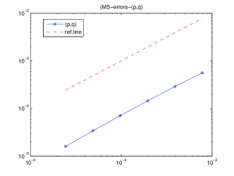
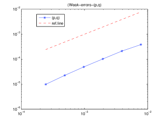
Fig. 1: Stochastic pendulum with $c_{1}=1$ and $c_{2}=0.5$. Left: Mean-square order, Right: Weak order. Endpoint errors versus decreasing step sizes $h$ in log-log scale. The reference lines have slope $1$.

Figure 1 displays the convergence order in both mean-square and weak sense. From Theorems 6 and 8, we know that the conservative scheme (2) is of order $1$ in the mean-square, resp. weak sense for this stochastic mathematical pendulum problem. The errors are computed at the endpoint $T_{N}=1$, the reference solution is computed using the step size $h_{\text{exact}}=2^{-14}$ and the expectation is realised using the average of $1000$ independent pathes. We can observe from Figure 1 (left) a mean-square order of convergence one for the conservative scheme (2). The right picture shows the convergence order of $|E\big{(}\psi(p(T_{N}),q(T_{N}))-\psi(p_{N},q_{N})\big{)}|$ with the function $\psi(p,q)=\sin(p)+q^{2}$. The reference line has slope $1$, and we observe that the convergence orders are consistent with our theoretical results.

6.2 Experiment 2

We are also interested in the following example, whose coefficients do not satisfy the hypotheses of our main theorems. However, numerical results show that the convergence orders still coincide with our theoretical assertions. We may say that our theory suits for a broader class of problems than we claimed, and the study for the optimal assumptions is an open problem. In order to illustrate this, we consider the cyclic Lotka-Volterra (with commutative noise) [16]

$$\text{d}\begin{pmatrix}x^{1}\\ x^{2}\\ x^{3}\end{pmatrix} =\begin{pmatrix}x^{1}(x^{3}-x^{2})\\ x^{2}(x^{1}-x^{3})\\ x^{3}(x^{2}-x^{1})\end{pmatrix}\text{d}t+\begin{pmatrix}x^{1}\\ x^{2}\\ -2x^{3}\end{pmatrix}\circ\text{d}W_{1}+\begin{pmatrix}x^{1}\\ -2x^{2}\\ x^{3}\end{pmatrix}\circ\text{d}W_{2}+\begin{pmatrix}-2x^{1}\\ x^{2}\\ x^{3}\end{pmatrix}\circ\text{d}W_{3}.$$

This problem has the conserved quantity $I(x)=x^{1}x^{2}x^{3}$ and possesses the following skew gradient form (2)

$$\text{d}\begin{pmatrix}x^{1}\\ x^{2}\\ x^{3}\end{pmatrix} =\begin{pmatrix}0&1&-1\\ -1&0&1\\ 1&-1&0\end{pmatrix}\nabla I(x)\,\text{d}t+\begin{pmatrix}0&\frac{1}{2x^{3}}&\frac{1}{2x^{2}}\\[5.69054pt] -\frac{1}{2x^{3}}&0&\frac{3}{2x^{1}}\\[5.69054pt] -\frac{1}{2x^{2}}&-\frac{3}{2x^{1}}&0\end{pmatrix}\nabla I(x)\circ\text{d}W_{1}$$

$$+\begin{pmatrix}0&\frac{1}{2x^{3}}&\frac{1}{2x^{2}}\\[5.69054pt] -\frac{1}{2x^{3}}&0&-\frac{3}{2x^{1}}\\[5.69054pt] -\frac{1}{2x^{2}}&\frac{3}{2x^{1}}&0\end{pmatrix}\nabla I(x)\circ\text{d}W_{2}+\begin{pmatrix}0&-\frac{1}{2x^{3}}&-\frac{1}{2x^{2}}\\[5.69054pt] \frac{1}{2x^{3}}&0&\frac{3}{2x^{1}}\\[5.69054pt] \frac{1}{2x^{2}}&-\frac{3}{2x^{1}}&0\end{pmatrix}\nabla I(x)\circ\text{d}W_{3}.$$

We will now numerically integrate this problem on the interval $[0,1]$ using the initial values $x_{0}=(0.01,0.01,0.01)^{T}$.

From Theorems 6 and 8, we know that the conservative scheme (2) is of order $1$ in the mean-square, resp. weak sense. Aiming at verifying these convergence orders, we compute the errors at the endpoint $T_{N}=1$, the expectation is realized using the average of $1000$ independent pathes. The left part of Figure 2 displays the mean-square errors. The lines with $*$ represent the relative errors $\displaystyle\frac{(E|y(T_{N})-y_{N}|^{2})^{1/2}}{(E|y(T_{N})|^{2})^{1/2}}$ with $y$ being $x^{1}$, $x^{2}$, $x^{3}$ or $x$. The right part of Figure 2 displays the weak errors. The lines with $*$ represents the relative errors $\displaystyle\frac{|E(\psi(y(T_{N}))-\psi(y_{N}))|}{|E\psi(y(T_{N}))|}$ with the function $\psi(x)$ being $x^{1}x^{2}$, $x^{2}x^{3}$, $(x^{1})^{2}$ or $|x|^{2}$. The reference solution $y(T_{N})$ is computed using the stochastic midpoint scheme with stepsize $h=2^{-14}$ and the numerical solutions $y_{N}$ are computed using method (2). We observe the desired convergence orders for the conservative scheme (2).

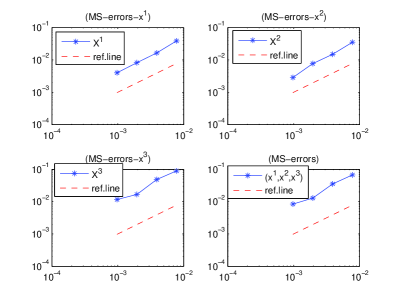
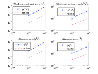
Fig. 2: (Conservative scheme (2). Left: Mean-square order, Right: Weak order) Endpoint errors versus decreasing step sizes $h$ in log-log scale for the stochastic cyclic Lotka-Volterra system. The reference lines have slope $1$.

We next repeat the same numerical experiments using the numerical method (4) with the classical midpoint rule. We obtain similar plots as in the above experiments thus confirming the convergence results from Theorems 10 and 11. The plots are however not presented.

We finally apply a composition scheme to the cyclic Lotka-Volterra system in order to verify the conclusions of Theorem 13. To do this, we choose the set $\Gamma=\{12,13,23\}$ and consider $V_{0}^{ij}=S^{ij}\partial_{j}I\partial i-S^{ji}\partial_{i}I\partial_{j}$ and $V_{r}^{ij}=T_{r}^{ij}\partial_{j}I\partial i-T_{r}^{ji}\partial_{i}I\partial_{j}$ for $\alpha=ij\in\Gamma$. For the above systems, the composition method (18) reads

$$Y_{n+1}=\bar{X}_{[12]}(\dfrac{1}{2})\circ\,\bar{X}_{[13]}(\dfrac{1}{2})\circ\,\bar{X}_{[23]}(1)\circ\,\bar{X}_{[13]}(\dfrac{1}{2})\circ\,\bar{X}_{[12]}(\dfrac{1}{2})\circ\,Y_{n}.$$

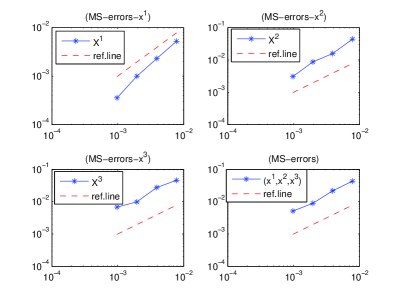
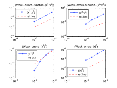
Fig. 3: (Composition method (18). Left: Mean-square order, Right: Weak order) Endpoint errors versus decreasing step sizes $h$ in log-log scale for the stochastic cyclic Lotka-Volterra system. The reference lines have slopes $1$.

The left part of Figure 3 presents the mean-square errors. The lines with $*$ represents the values of $\displaystyle\frac{(E|y(T_{N})-y_{N}|^{2})^{1/2}}{(E|y(T_{N})|^{2})^{1/2}}$ with $y$ being $x^{1}$, $x^{2}$, $x^{3}$ or $x$. The right part of Figure 3 presents the weak errors. The lines with $*$ represents the values of $\displaystyle\frac{|E(\psi(y(T_{N}))-\psi(y_{N}))|}{|E\psi(y(T_{N}))|}$ with the function $\psi(x)$ being $x^{1}x^{2}$, $x^{2}x^{3}$, $(x^{1})^{2}$ or $|x|^{2}$. Again, the correct convergence orders are observed.

7 Conclusion

Based on the energy-preserving method for stochastic Poisson system [6] and the equivalent skew gradient system formulation of the original system [9], we present a new invariant-preserving method for general stochastic differential equations in the Stratonovich sense with a conserved quantity. We show that the invariant-preserving method converges with accuracy order $1$ for commutative noise in mean-square sense. In the commutative as well as non-commutative case, the weak convergence order of the proposed method is $1$. Influences of the usage of a quadrature formula on the orders of convergence are also investigated. Further, a conservative composition method is studied: mean-square convergence order $1$ for commutative noise and weak convergence order $1$ are obtained. Finally, numerical experiments are presented to verify extend our theoretical results. We will study multiple invariants-preserving methods for stochastic differential equations in a future work.

References

- [1] A. Abdulle, D. Cohen, G. Vilmart, and K.C. Zygalakis. High order weak methods for stochastic differential equations based on modified equations. SIAM J. Sci. Comp., 34, A1800–A1823 (2012).
- [2] J.-M. Bismut. Mécanique Aléatoire, volume 866. Springer-Verlag, 1981.
- [3] K. Burrage and P. M. Burrage. Order conditions of stochastic Runge-Kutta methods by -series. SIAM J. Numer. Anal., 38, 1626–1646 (2000).
- [4] K. Burrage, P. M. Burrage, and T. Tian. Numerical methods for strong solutions of stochastic differential equations: an overview. Proc. R. Soc. Lond. Ser. A Math. Phys. Eng. Sci., 460, 373–402 (2004). Stochastic analysis with applications to mathematical finance.
- [5] D. Cohen. On the numerical discretisation of stochastic oscillators. Math. Comp. Simul., 82, 1478–1495 (2012).
- [6] D. Cohen and G Dujardin. Energy-preserving integrators for stochastic Poisson systems. Accepted for publication in Commun. Math. Sci., 2013.
- [7] E. Faou and T. Lelièvre. Conservative stochastic differential equations: mathematical and numerical analysis. Math. Comp., 78, 2047–2074 (2009).
- [8] G.W. Gardiner. Handbook of stochastic processes for physics, chemistry and natural sciences. Springer Verlag, 2 edition, 1985.
- [9] J. Hong, S. Zhai, and J. Zhang. Discrete gradient approach to stochastic differential equations with a conserved quantity. SIAM J. Numer. Anal., 49, 2017–2038 (2011).
- [10] P. E. Kloeden and E. Platen. Numerical Solution of Stochastic Differential Equations, volume 23 of Applications of Mathematics (New York). Springer-Verlag, Berlin, 1992.
- [11] S. J. A. Malham and A. Wiese. Stochastic Lie group integrators. SIAM J. Sci. Comput., 30, 597–617 (2008).
- [12] G. N. Milstein, Yu. M. Repin, and M. V. Tretyakov. Mean-square symplectic methods for Hamiltoninan systems with multiplicative noise. WIAS preprint, 670, (2001).
- [13] G. N. Milstein, Yu. M. Repin, and M. V. Tretyakov. Numerical methods for stochastic systems preserving symplectic structure. SIAM J. Numer. Anal., 40, 1583–1604 (2002) (electronic).
- [14] G. N. Milstein, Yu. M. Repin, and M. V. Tretyakov. Symplectic integration of Hamiltonian systems with additive noise. SIAM J. Numer. Anal., 39, 2066–2088 (electronic) (2002) (electronic).
- [15] G. N. Milstein and M. V. Tretyakov. Stochastic Numerics for Mathematical Physics. Scientific Computation. Springer-Verlag, Berlin, 2004.
- [16] T. Misawa. Conserved quantities and symmetries related to stochastic dynamical systems. Ann. Inst. Statist. Math., 51, 779–802 (1999).
- [17] T. Misawa. Energy conservative stochastic difference scheme for stochastic Hamilton dynamical systems. Japan J. Indust. Appl. Math., 17, 119–128 (2000).
- [18] T. Misawa. Numerical integration of stochastic differential equations by composition methods. Sūrikaisekikenkyūsho Kōkyūroku, (1180),166–190, 2000. Dynamical systems and differential geometry (Japanese) (Kyoto, 2000).
- [19] E. Moro and H. Schurz. Boundary preserving semianalytic numerical algorithms for stochastic differential equations. SIAM J. Sci. Comput., 29, 1525–1549 (electronic) (2007) (electronic).
- [20] S.T. Rachev (e.d.). Handbook of computational and numerical methods in finance. Birkhauser, Boston, 2004.
- [21] A. Rößler. Runge-Kutta methods for Stratonovich stochastic differential equation systems with commutative noise. In Proceedings of the 10th International Congress on Computational and Applied Mathematics (ICCAM-2002), 164/165, 613–627 (2004).
- [22] H. Schurz. The invariance of asymptotic laws of linear stochastic systems under discretization. ZAMM Z. Angew. Math. Mech., 79, 375–382 (1999).
- [23] H. Schurz. Preservation of probabilistic laws through Euler methods for Ornstein-Uhlenbeck process. Stochastic Anal. Appl., 17, 463–486 (1999).
- [24] P.D. Spanos (e.d.). Computational stochastic mechanics. Balkema, Rotterdam, Netherlands, 1999.
- [25] D. Talay. Efficient numerical schemes for the approximation of expectations of functionals of the solution of a SDE and applications. In Filtering and control of random processes (Paris, 1983), volume 61 of Lecture Notes in Control and Inform. Sci., pages 294–313. Springer, Berlin, 1984.
- [26] L. Wang, J. Hong, R. Scherer, and F. Bai. Dynamics and variational integrators of stochastic Hamiltonian systems. Int. J. Numer. Anal. Model., 6, 586–602 (2009).