Introduction to the R package TDA

Abstract

We present a short tutorial and introduction to using the R package TDA, which provides some tools for Topological Data Analysis. In particular, it includes implementations of functions that, given some data, provide topological information about the underlying space, such as the distance function, the distance to a measure, the kNN density estimator, the kernel density estimator, and the kernel distance. The salient topological features of the sublevel sets (or superlevel sets) of these functions can be quantified with persistent homology. We provide an R interface for the efficient algorithms of the C++ libraries GUDHI, Dionysus and PHAT, including a function for the persistent homology of the Rips filtration, and one for the persistent homology of sublevel sets (or superlevel sets) of arbitrary functions evaluated over a grid of points. The significance of the features in the resulting persistence diagrams can be analyzed with functions that implement recently developed statistical methods. The R package TDA also includes the implementation of an algorithm for density clustering, which allows us to identify the spatial organization of the probability mass associated to a density function and visualize it by means of a dendrogram, the cluster tree.

1 Introduction

Topological Data Analysis (TDA) refers to a collection of methods for finding topological structure in data (Carlsson, 2009). Recent advances in computational topology have made it possible to actually compute topological invariants from data. The input of these procedures typically takes the form of a point cloud, regarded as possibly noisy observations from an unknown lower-dimensional set $S$ whose interesting topological features were lost during sampling. The output is a collection of data summaries that are used to estimate the topological features of $S$.

One approach to TDA is persistent homology (Edelsbrunner and Harer, 2010), a method for studying the homology at multiple scales simultaneously. More precisely, it provides a framework and efficient algorithms to quantify the evolution of the topology of a family of nested topological spaces. Given a real-valued function $f$, such as the ones described in Section 2, persistent homology describes how the topology of the lower level sets $\{x:f(x)\leq t\}$ (or superlevel sets $\{x:f(x)\geq t\}$) change as $t$ increases from $-\infty$ to $\infty$ (or decreases from $\infty$ to $-\infty$). This information is encoded in the persistence diagram, a multiset of points in the plane, each corresponding to the birth-time and death-time of a homological feature that exists for some interval of $t$.

This paper is devoted to the presentation of the R package TDA, which provides a user-friendly interface for the efficient algorithms of the C++ libraries GUDHI (Maria, 2014), Dionysus (Morozov, 2007), and PHAT (Bauer et al., 2012). The package can be downloaded from http://cran.r-project.org/web/packages/TDA/index.html.

In Section 2, we describe how to compute some widely studied functions that, starting from a point cloud, provide topological information about the underlying space: the distance function (distFct), the distance to a measure function (dtm), the k Nearest Neighbor density estimator (knnDE), the kernel density estimator (kde), and the kernel distance (kernelDist). Section 3 is devoted to the computation of persistence diagrams: the function gridDiag can be used to compute persistent homology of sublevel sets (or superlevel sets) of functions evaluated over a grid of points; the function ripsDiag returns the persistence diagram of the Rips filtration built on top of a point cloud.

One of the key challenges in persistent homology is to find a way to separate the points of the persistence diagram representing the topological noise from the points representing the topological signal. Statistical methods for persistent homology provide an alternative to its exact computation. Knowing with high confidence that an approximated persistence diagram is close to the true–computationally infeasible–diagram is often enough for practical purposes. Fasy et al. (2014), Chazal et al. (2014c), and Chazal et al. (2014a) propose several statistical methods to construct confidence sets for persistence diagrams and other summary functions that allow us to separate topological signal from topological noise. The methods are implemented in the TDA package, and described in Section 3.

Finally, the TDA package provides the implementation of an algorithm for density clustering. This method allows us to identify and visualize the spatial organization of the data, without specific knowledge about the data generating mechanism and in particular without any a priori information about the number of clusters. In Section 4, we describe the function clusterTree, that, given a density estimator, encodes the hierarchy of the connected components of its superlevel sets into a dendrogram, the cluster tree (Kpotufe and von Luxburg, 2011; Kent, 2013).

2 Distance Functions and Density Estimators

As a first example illustrating how to use the TDA package, we show how to compute distance functions and density estimators over a grid. The setting is the typical one in TDA: a set of points $X=\{x_{1},\dots,x_{n}\}\subset\mathbb{R}^{d}$ has been sampled from some distribution $P$ and we are interested in recovering the topological features of the underlying space by studying some functions of the data. The following code generates a sample of 400 points from the unit circle and constructs a grid over which we will evaluate the functions.

.

> library("TDA")> X = circleUnif(400)> Xlim=c(-1.6, 1.6);   Ylim=c(-1.7, 1.7);   by=0.065> Xseq=seq(Xlim[1], Xlim[2], by=by)> Yseq=seq(Ylim[1], Ylim[2], by=by)> Grid=expand.grid(Xseq,Yseq).

The TDA package provides implementations of the following functions:

1. The distance function is defined for each $y\in\mathbb{R}^{d}$ as $\Delta(y)=\inf_{x\in X}\|x-y\|_{2}$ and is computed for each point of the Grid with the following code:

   .

   > distance = distFct(X=X, Grid=Grid).

2. Given a probability measure $P$ on ${\mathbb{R}}^{d}$, the distance-to-a-measure (DTM) is defined for each $y\in\mathbb{R}^{d}$ as

   $$d_{m_{0}}(y)=\sqrt{\frac{1}{m_{0}}\int_{0}^{m_{0}}(G_{y}^{-1}(u))^{2}du},$$

   where $G_{y}(t)=P(\|X-y\|\leq t)$ and $0<m_{0}<1$ is a smoothing parameter. The DTM can be seen as a smoothed version of the distance function. For more details, see Chazal et al. (2011).

   Given $X=\{x_{1},\dots,x_{n}\}\subset{\mathbb{R}}^{d}$, the empirical version of the DTM is

   $$\hat{d}_{m_{0}}(y)=\sqrt{\frac{1}{k}\sum_{x_{i}\in N_{k}(y)}\|x_{i}-y\|^{2}},$$

   where $k=\lceil m_{0}n\rceil$ and $N_{k}(y)$ is the set containing the $k$ nearest neighbors of $y$ among $x_{1},\ldots,x_{n}$. The DTM is computed for each point of the Grid with the following code:

   .

   > m0=0.1> DTM=dtm(X=X, Grid=Grid, m0=m0).

3. The $k$ Nearest Neighbor density estimator, for each $y\in\mathbb{R}^{d}$, is defined as

   $$\hat{\delta}_{k}(y)=\frac{k}{n\;v_{d}\;r_{k}^{d}(y)},$$

   where $v_{d}$ is the volume of the Euclidean $d$-dimensional unit ball and $r_{k}(x)$ is the Euclidean distance form point $x$ to its $k$th closest neighbor among the points of $X$. It is computed for each point of the Grid with the following code:

   .

   > k=60> kNN=knnDE(X=X, Grid=Grid, k=k).

4. The Gaussian Kernel Density Estimator (KDE), for each $y\in\mathbb{R}^{d}$, is defined as

   $$\hat{p}_{h}(y)=\frac{1}{n(\sqrt{2\pi}h)^{d}}\sum_{i=1}^{n}\exp\left(\frac{-\|y-x_{i}\|_{2}^{2}}{2h^{2}}\right).$$

   where $h$ is a smoothing parameter. It is computed for each point of the Grid with the following code:

   .

   > h=0.3> KDE= kde(X=X, Grid=Grid, h=h).

5. The Kernel distance estimator, for each $y\in\mathbb{R}^{d}$, is defined as

   $$\hat{\kappa}_{h}(y)=\sqrt{\frac{1}{n^{2}}\sum_{i=1}^{n}\sum_{j=1}^{n}K_{h}(x_{i},x_{j})+K_{h}(y,y)-2\frac{1}{n}\sum_{i=1}^{n}K_{h}(y,x_{i})},$$

   where $K_{h}(x,y)=\exp\left(\frac{-\|x-y\|_{2}^{2}}{2h^{2}}\right)$ is the Gaussian Kernel with smoothing parameter $h$. The Kernel distance is computed for each point of the Grid with the following code:

   .

   > h=0.3> Kdist= kernelDist(X=X, Grid=Grid, h=h).

For this two-dimensional example, we can visualize the functions using persp form the graphics package. For example the following code produces the KDE plot in Figure 1:

.

> persp(Xseq,Yseq,matrix(KDE,ncol=length(Yseq), nrow=length(Xseq)),+ xlab="",ylab="",zlab="",theta=-20,phi=35, ltheta=50, col=2, border=NA,+ main="KDE", d=0.5, scale=FALSE, expand=3, shade=0.9).

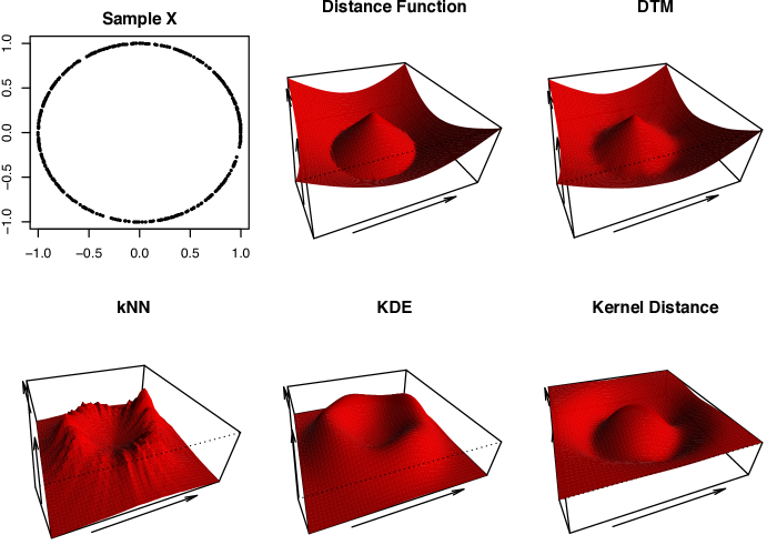
Figure 1: distance functions and density estimators evaluated over a grid of points.

2.1 Bootstrap Confidence Bands

We can construct a $(1-\alpha)$ confidence band for a function using the bootstrap algorithm, which we briefly describe using the kernel density estimator:

1. Given a sample $X=\{x_{1},\dots,x_{n}\}$, compute the kernel density estimator $\hat{p}_{h}$;

2. Draw $X^{*}=\{x_{1}^{*},\dots,x_{n}^{*}\}$ from $X=\{x_{1},\dots,x_{n}\}$ (with replacement), and compute $\theta^{*}=\sqrt{n}\|\hat{p}_{h}^{*}(x)-\hat{p}_{h}(x)\|_{\infty}$, where $\hat{p}_{h}^{*}$ is the density estimator computed using $X^{*}$;

3. Repeat the previous step $B$ times to obtain $\theta_{1}^{*},\dots,\theta_{B}^{*}$;

4. Compute $q_{\alpha}=\inf\left\{q:\frac{1}{B}\sum_{j=1}^{B}I(\theta_{j}^{*}\geq q)\leq\alpha\right\};$

5. The $(1-\alpha)$ confidence band for $\mathbb{E}[\hat{p}_{h}]$ is $\left[\hat{p}_{h}-\frac{q_{\alpha}}{\sqrt{n}}\,,\,\hat{p}_{h}+\frac{q_{\alpha}}{\sqrt{n}}\right].$

Fasy et al. (2014) and Chazal et al. (2014a) prove the validity of the bootstrap algorithm for kernel density estimators, distance-to-a-measure, and kernel distance, and use it in the framework of persistent homology. The bootstrap algorithm is implemented in the function bootstrapBand, which provides the option of parallelizing the algorithm (parallel=TRUE) using the package parallel. The following code computes a 90% confidence band for $\mathbb{E}[\hat{p}_{h}]$, showed in Figure 2.

.

> band=bootstrapBand(X=X, FUN=kde, Grid=Grid, B=100,+                    parallel=FALSE, alpha=0.1, h=h).

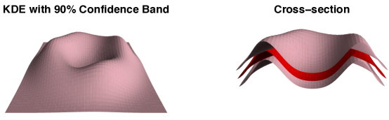
Figure 2: the 90% confidence band for $\mathbb{E}[\hat{p}_{h}]$ has the form $[\ell,u]=\left[\hat{p}_{h}-q_{\alpha}/\sqrt{n}\,,\,\hat{p}_{h}+q_{\alpha}/\sqrt{n}\right]$. The plot on the right shows a cross-section of the functions: the red surface is the KDE $\hat{p}_{h}$; the pink surfaces are $\ell$ and $u$.

3 Persistent Homology

We provide an informal description of the implemented methods of persistent homology. We assume the reader is familiar with the basic concepts and, for a rigorous exposition, we refer to the textbook Edelsbrunner and Harer (2010).

3.1 Persistent Homology Over a Grid

In this section, we describe how to use the gridDiag function to compute the persistent homology of sublevel (and superlevel) sets of the functions described in Section 2. The function gridDiag evaluates a given real valued function over a triangulated grid, constructs a filtration of simplices using the values of the function, and computes the persistent homology of the filtration. From version 1.2, gridDiag works in arbitrary dimension. The core of the function is written in C++ and the user can choose to compute persistence diagrams using either the Dionysus library or the PHAT library.

The following code computes the persistent homology of the superlevel sets (sublevel=FALSE) of the kernel density estimator (FUN=kde, h=0.3) using the point cloud stored in the matrix X from the previous example. The same code would work for the other functions defined in Section 2 (it is sufficient to replace kde and its smoothing parameter h with another function and the corresponding parameter). The function gridDiag returns an object of the class "diagram". The other inputs are the features of the grid over which the kde is evaluated (lim and by), the smoothing parameter h, and a logical variable that indicates whether a progress bar should be printed (printProgress).

.

> Diag = gridDiag( X=X, FUN=kde, h=0.3, lim=cbind(Xlim,Ylim), by=by,+                  sublevel=F, library="Dionysus", printProgress=FALSE )$diagram.

We plot the data and the diagram, using the function plot, implemented as a standard S3 method for objects of the class "diagram". The following command produces the third plot in Figure 3.

.

> plot(Diag, band=2*band$width, main="KDE Diagram").

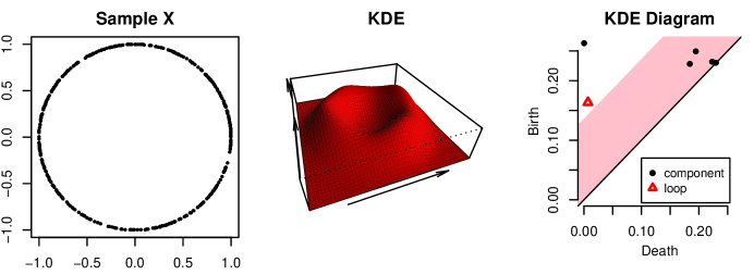
Figure 3: The plot on the right shows the persistence diagram of the superlevel sets of the KDE. Black points represent connected components and red triangles represent loops. The features are born at high levels of the density and die at lower levels. The pink 90% confidence band separates significant features from noise.

The option band=2*band$width produces a pink confidence band for the persistence diagram, using the confidence band constructed for the corresponding kernel density estimator in the previous section. The features above the band can be interpreted as representing significant homological features, while points in the band are not significantly different from noise. The validity of the bootstrap confidence band for persistence diagrams of KDE, DTM, and Kernel Distance derive from the Stability Theorem (Chazal et al., 2012) and is discussed in detail in Fasy et al. (2014) and Chazal et al. (2014a).

The function plot for the class "diagram" provides the options of rotating the diagram (rotated=TRUE), drawing the barcode in place of the diagram (barcode=TRUE), as well as other standard graphical options. See Figure 4.

.

> par(mfrow=c(1,2), mai=c(0.8,0.8,0.3,0.1))

> plot(Diag, rotated=T, band=band$width, main="Rotated Diagram")

> legend(0.13,0.25, c("component", "loop"), col=c(1,2), pch=c(20,2), cex=0.9, pt.lwd=2)

> plot(Diag, barcode=T,  main="Barcode")

.

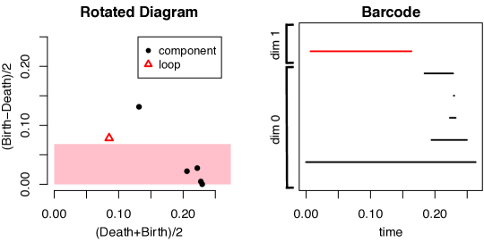
Figure 4: Rotated Persistence Diagram and Barcode

3.2 Rips Diagrams

The Vietoris-Rips complex $R(X,\varepsilon)$ consists of simplices with vertices in $X=\{x_{1},\dots,x_{n}\}\subset\mathbb{R}^{d}$ and diameter at most $\varepsilon$. In other words, a simplex $\sigma$ is included in the complex if each pair of vertices in $\sigma$ is at most $\varepsilon$ apart. The sequence of Rips complexes obtained by gradually increasing the radius $\varepsilon$ creates a filtration.

The ripsDiag function computes the persistence diagram of the Rips filtration built on top of a point cloud. The user can choose to compute the Rips persistence diagram using either the C++ library GUDHI, or Dionysus.
The following code generates 60 points from two circles:

.

> Circle1 = circleUnif(60)> Circle2 = circleUnif(60, r=2) +3> Circles=rbind(Circle1,Circle2).

We specify the limit of the Rips filtration and the maximum dimension of the homological features we are interested in (0 for components, 1 for loops, 2 for voids, etc.):

.

> maxscale=5           # limit of the filtration> maxdimension=1       # components and loops.

and we generate the persistence diagram:

.

> Diag=ripsDiag(X=Circles, maxdimension, maxscale,+               library="GUDHI", printProgress=FALSE)$diagram. Alternatively, using the option dist="arbitrary" in ripsDiag(), the input X can be an $n\times n$ matrix of distances. This option is useful when the user wants to consider a Rips filtration constructed using an arbitrary distance and is currently only available for the option library="Dionysus".

Finally, we plot the data and the diagram:

.

> par(mfrow=c(1,2), mai=c(0.8,0.8,0.3,0.1))

> plot(Circles, pch=16, xlab="",ylab="", main="Sample")

> plot(Diag, main="Rips Diagram")

> legend(2.5,2, c("component", "loop"), col=c(1,2), pch=c(20,2), cex=0.9, pt.lwd=2)

.

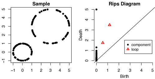
Figure 5: Rips persistence diagram. Black points represent connected components and red triangles represent loops.

3.3 Bottleneck and Wasserstein Distances

Standard metrics for measuring the distance between two persistence diagrams are the bottleneck distance and the $p$th Wasserstein distance (Edelsbrunner and Harer, 2010). The TDA package includes the functions bottleneck and wasserstein, which are R wrappers of the Dionysus functions “bottleneck_distance" and “wasserstein_distance."

We generate two persistence diagrams of the Rips filtrations built on top of the two (separate) circles of the previous example,

.

> Diag1=ripsDiag(Circle1,maxdimension=1, maxscale=5, printProgress=FALSE)$diagram> Diag2=ripsDiag(Circle2,maxdimension=1, maxscale=5, printProgress=FALSE)$diagram. and we compute the bottleneck distance and the $2$nd Wasserstein distance between the two diagrams. In the following code, the option dimension=1 specifies that the distances between diagrams are computed using only one-dimensional homological features (loops).

.

> print( bottleneck(Diag1, Diag2, dimension=1) )

[1] 1.15569

> print( wasserstein(Diag1, Diag2, p=2, dimension=1) )

[1] 1.680847.

3.4 Landscapes and Silhouettes

Persistence landscapes and silhouettes are real-valued functions that further summarize the information contained in a persistence diagram. They have been introduced and studied in Bubenik (2012), Chazal et al. (2014c), and Chazal et al. (2014b). We briefly introduce the two functions.

Landscape. The persistence landscape is a sequence of continuous, piecewise linear functions $\lambda\colon\mathbb{Z}^{+}\times\mathbb{R}\to\mathbb{R}$ that provide an encoding of a persistence diagram. To define the landscape, consider the set of functions created by tenting each point $x=(x_{1},x_{2})=\left(\frac{b+d}{2},\frac{d-b}{2}\right)$ representing a birth-death pair $(b,d)$ in the persistence diagram $D$ as follows:

$$\Lambda_{p}(t)=\begin{cases}t-x_{1}+x_{2}&t\in[x_{1}-x_{2},x_{1}]\\ x_{1}+x_{2}-t&t\in(x_{1},x_{1}+x_{2}]\\ 0&\text{otherwise}\end{cases}=\begin{cases}t-b&t\in[b,\frac{b+d}{2}]\\ d-t&t\in(\frac{b+d}{2},d]\\ 0&\text{otherwise}.\end{cases}$$ (1)

We obtain an arrangement of piecewise linear curves by overlaying the graphs of the functions $\{\Lambda_{x}\}_{x}$; see Figure 6 (left). The persistence landscape of $D$ is a summary of this arrangement. Formally, the persistence landscape of $D$ is the collection of functions

$$\lambda(k,t)=\underset{x}{k\text{max}}~{}\Lambda_{x}(t),\quad t\in[0,T],k\in\mathbb{N},$$ (2)

where $k$max is the $k$th largest value in the set; in particular, $1$max is the usual maximum function. see Figure 6 (middle).

Silhouette. Consider a persistence diagram with $N$ off diagonal points $\{(b_{j},d_{j})\}_{j=1}^{N}$. For every $0<p<\infty$ we define the power-weighted silhouette

$$\phi^{(p)}(t)=\frac{\sum_{j=1}^{N}|d_{j}-b_{j}|^{p}\Lambda_{j}(t)}{\sum_{j=1}^{N}|d_{j}-b_{j}|^{p}}.$$

The value $p$ can be thought of as a trade-off parameter between uniformly treating all pairs in the persistence diagram and considering only the most persistent pairs. Specifically, when $p$ is small, $\phi^{(p)}(t)$ is dominated by the effect of low persistence features. Conversely, when $p$ is large, $\phi^{(p)}(t)$ is dominated by the most persistent features; see Figure 6 (right).

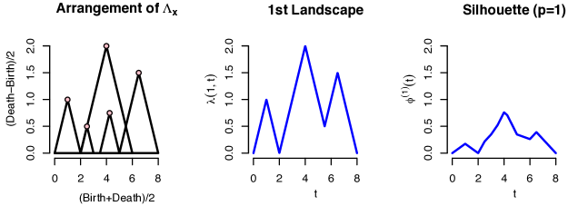
Figure 6: Left: we use the rotated axes to represent a persistence diagram $D$. A feature $(b,d)\in D$ is represented by the point $(\frac{b+d}{2},\frac{d-b}{2})$ (pink). In words, the $x$-coordinate is the average parameter value over which the feature exists, and the $y$-coordinate is the half-life of the feature. Middle: the blue curve is the landscape $\lambda(1,\cdot)$. Right: the blue curve is the silhouette $\phi^{(1)}(\cdot)$.

The landscape and silhouette functions can be evaluated over a one-dimensional grid of points tseq using the functions landscape and silhouette. In the following code, we use the persistence diagram from Figure 5 to construct the corresponding landscape and silhouette for one-dimensional features (dimension=1). The option KK=1 specifies that we are interested in the 1st landscape function, and p=1 is the power of the weights in the definition of the silhouette function.

.

> tseq=seq(0,maxscale, length=1000)   #domain> Land= landscape(Diag, dimension=1, KK=1, tseq)> Sil=silhouette(Diag, p=1,  dimension=1, tseq).

The functions landscape and silhouette return real valued vectors, which can be simply plotted with plot(tseq, Land, type="l"); plot(tseq, Sil, type="l"). See Figure 7.

Figure 7: Landscape and Silhouette of the one-dimensional features of the diagram of Figure 5.

3.5 Confidence Bands for Landscapes and Silhouettes

Recent results in Chazal et al. (2014c) and Chazal et al. (2014b) show how to construct confidence bands for landscapes and silhouettes, using a bootstrap algorithm (specifically, the multiplier bootstrap). This strategy is useful in the following scenario. We have a very large dataset with $N$ points. There is a diagram $D$ and landscape $\lambda$ corresponding to some filtration built on the data. When $N$ is large, computing $D$ is prohibitive. Instead, we draw $n$ subsamples, each of size $m$. We compute a diagram and a landscape for each subsample yielding landscapes $\lambda_{1},\dots,\lambda_{n}$. (Assuming $m$ is much smaller than $N$, these subsamples are essentially independent and identically distributed.) Then we compute $\frac{1}{n}\sum_{i}\lambda_{i}$, an estimate of $\mathbb{E}(\lambda_{i})$, which can be regarded as an approximation of $\lambda$. The function multipBootstrap uses the landscapes $\lambda_{1},\dots,\lambda_{n}$ to construct a confidence band for $\mathbb{E}(\lambda_{i})$. The same strategy is valid for silhouette functions. We illustrate the method with a simple example.
First we sample $N$ points from two circles:

.

> N=4000> XX1 = circleUnif(N/2)> XX2 = circleUnif(N/2, r=2) +3> X=rbind(XX1,XX2).

Then we specify the number of subsamples $n$, the subsample size $m$, and we create the objects that will store the $n$ diagrams and landscapes:

.

> m=80        # subsample size> n=10        # we will compute n landscapes using subsamples of size m> tseq=seq(0,maxscale, length=500)          #domain of landscapes> Diags=list()                              #here we store n Rips diags> Lands=matrix(0,nrow=n, ncol=length(tseq)) #here we store n landscapes.

For $n$ times, we subsample from the large point cloud, compute $n$ Rips diagrams and the corresponding 1st landscape functions (KK=1), using one-dimensional features (dimension=1):

.

> for (i in 1:n){+ subX=X[sample(1:N,m),]+ Diags[[i]]=ripsDiag(subX,maxdimension=1, maxscale=5)$diagram+ Lands[i,]=landscape(Diags[[i]], dimension=1, KK=1, tseq )+ }.

Finally we use the $n$ landscapes to construct a 95% confidence band for the mean landscape

.

> bootLand=multipBootstrap(Lands,B=100,alpha=0.05, parallel=FALSE). which is plotted by the following code. See Figure 8.

.

> plot(tseq, bootLand$mean, main="Mean Landscape with 95% band")> polygon(c(tseq, rev(tseq)),+         c(bootLand$band[,1],rev(bootLand$band[,2])), col="pink")> lines(tseq, bootLand$mean, lwd=2, col=2).

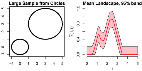
Figure 8: 95% confidence band for the mean landscape function.

3.6 Selection of Smoothing Parameters

An unsolved problem in topological inference is how to choose the smoothing parameters, for example $h$ for KDE and $m_{0}$ for DTM.

Chazal et al. (2014a) suggest the following method, that we describe here for the kernel density estimator, but works also for the kernel distance and the distance-to-a-measure.

Let $\ell_{1}(h),\ell_{2}(h),\ldots,$ be the lifetimes of the features of a persistence diagram at scale $h$. Let $q_{\alpha}(h)/\sqrt{n}$ be the width of the confidence band for the kernel density estimator at scale $h$, as described in Section 2.1. We define two quantities that measure the amount of significant information at level $h$:

• The number of significant features, $N(h)=\#\left\{i:\ \ell(i)>2\frac{q_{\alpha}(h)}{\sqrt{n}}\right\}$;

• The total significant persistence, $S(h)=\sum_{i}\left[\ell_{i}-2\frac{q_{\alpha}(h)}{\sqrt{n}}\right]_{+}$.

These measures are small when $h$ is small since $q_{\alpha}(h)$ is large. On the other hand, they are small when $h$ is large since all of the features of the KDE smooth out. Thus we have a kind of topological bias-variance tradeoff. We choose $h$ to maximize $N(h)$ or $S(h)$.

The method is implemented in the function maxPersistence, as illustrated in the following example. First, we sample 1600 points from two circles (plus some clutter noise) and we specify the limits of the grid over which the KDE is evaluated:

.

> XX1 = circleUnif(600)> XX2 = circleUnif(1000, r=1.5) +2.5> noise=cbind(runif(80, -2,5),runif(80, -2,5))> X=rbind(XX1,XX2, noise)> # Grid limits> Xlim=c(-2,5)> Ylim=c(-2,5)> by=0.2.

Then we specify a sequence of smoothing parameters among which we will select the optimal one, the number of bootstrap iterations and the level of the confidence bands to be computed:

.

> parametersKDE=seq(0.1,0.6,by=0.05)> B=50        # number of bootstrap iterations. Should be large.> alpha=0.1   # level of the confidence bands.

The function maxPersistence can be parallelized (parallel=TRUE) and a progress bar can be printed (printProgress=TRUE):

.

> maxKDE=maxPersistence(kde, parametersKDE, X, lim=cbind(Xlim, Ylim),+                    by=by, sublevel=F, B=B, alpha=alpha,+                    parallel=TRUE, bandFUN="bootstrapBand").

The S3 methods summary and plot are implemented for the class "maxPersistence". We can display the values of the parameters that maximize the two criteria:

.

> print(summary(maxKDE))

Call:maxPersistence(FUN = kde, parameters = parametersKDE, X = X,    lim = cbind(Xlim, Ylim), by = by, sublevel = F, B = B, alpha = alpha,    bandFUN = "bootstrapBand", parallel = TRUE)The number of significant features is maximized by[1] 0.20 0.25 0.30The total significant persistence is maximized by[1] 0.1. and produce the summary plot of Figure 9.

.

> par(mfrow=c(1,2), mai=c(0.8,0.8,0.35,0.3))

> plot(X, pch=16, cex=0.5, main="Two Circles + Noise", xlab="", ylab="")

> plot(maxKDE, main="Max Persistence (KDE)")

.

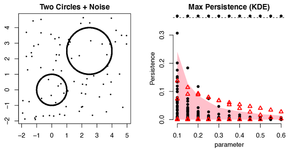
Figure 9: Max Persistence Method for the selection of smoothing parameters. For each value of the smoothing parameter we display the persistence of the corresponding homological features, along with a (pink) confidence band that separates the statistically significant features from the topological noise.

4 Density Clustering

The final example of this paper demonstrates the use of the function clusterTree, which is an implementation of Algorithm 1 in Kent et al. (2013).

First, we briefly describe the task of density clustering; we defer the reader to Kent (2013) for a more rigorous and complete description. Let $f$ be the density of the probability distribution $P$ generating the observed sample $X=\{x_{1},\dots,x_{n}\}\subset\mathbb{R}^{d}$. For a threshold value $\lambda>0$, the corresponding super level set of $f$ is $L_{f}(\lambda):=\text{cl}(\{x\in\mathbb{R}^{s}:f(x)>\lambda\})$, and its $d$-dimensional subsets are called high-density regions. The high-density clusters of $P$ are the maximal connected subsets of $L_{f}(\lambda)$. By considering all the level sets simultaneously (from $\lambda=0$ to $\lambda=\infty$), we can record the evolution and the hierarchy of the high-density clusters of $P$. This naturally leads to the notion of the cluster density tree of $P$ (see, e.g., Hartigan (1981)), defined as the collection of sets $T:=\{L_{f}(\lambda),\lambda\geq 0\}$, which satisfies the tree property: $A,B\in T$ implies that $A\subset B$ or $B\subset A$ or $A\cap B=\emptyset$. We will refer to this construction as the $\lambda$-tree. Alternatively, Kent et al. (2013) introduced the $\alpha$-tree and the $\kappa$-tree, which facilitate the interpretation of the tree by precisely encoding the probability content of each tree branch rather than the density level. Cluster trees are particularly useful for high-dimensional data, whose spatial organization is difficult to represent.

We illustrate the strategy with a simple example. The first step is to generate a 2D point cloud from three (not so well) separated clusters (see top left plot of Figure 10):

.

> X1=cbind(rnorm(300,1,.8),rnorm(300,5,0.8))> X2=cbind(rnorm(300,3.5,.8),rnorm(300,5,0.8))> X3=cbind(rnorm(300,6,1),rnorm(300,1,1))> XX=rbind(X1,X2,X3).

Then, we use the function clusterTree to compute cluster trees using the k Nearest Neighbors density estimator (density="knn", k=100 nearest neighbors).

.

> Tree=clusterTree(XX, k=100, density="knn").

Alternatively, we can estimate the density using a Gaussian kernel density estimator (density="kde", h=0.3 for the smoothing parameter). Even when the KDE is used to estimate the density, we have to provide the option k=100, so that the algorithm can compute the connected components at each level of the density using a k Nearest Neighbors graph.

The "clusterTree" object Tree contains information about the $\lambda$-tree, $\alpha$-tree and $\kappa$-tree. The function plot for objects of the class "clusterTree" produces the plot in the middle of Figure 10.

.

> plot(Tree, type="lambda", main="lambda Tree (knn)").

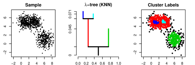
Figure 10: The $\lambda$-tree of the k Nearest Neighbor density estimator.

5 Conclusions

The TDA package makes topological data analysis accessible to a larger audience by providing access to the efficient algorithms for the computation of persistent homology from the C++ libraries GUDHI, Dionysus, and PHAT to R users. Moreover, the package includes the implementation of an algorithm for density clustering and a series of tools for the statistical analysis of persistent homology, including the methods described in Fasy et al. (2014), Chazal et al. (2014c), and Chazal et al. (2014a).

We would like TDA to become a comprehensive assistant for the analysis of data from a topological point of view. The package will keep providing an R interface for the most efficient libraries for TDA and we plan to include new functionalities for all the steps in the data analysis process: new tools for summarizing the topological information contained in the data, methods for the statistical analysis of the summaries, and functions for displaying the results.

References

- Bauer et al. (2012) Bauer, U., Kerber, M., Reininghaus, J., 2012. PHAT, a software library for persistent homology. https://code.google.com/p/phat/.
- Bubenik (2012) Bubenik, P., 2012. Statistical topological data analysis using persistence landscapes. arXiv preprint arXiv:1207.6437.
- Carlsson (2009) Carlsson, G., 2009. Topology and data. Bulletin of the American Mathematical Society 46 (2), 255–308.
- Chazal et al. (2011) Chazal, F., Cohen-Steiner, D., Mérigot, Q., 2011. Geometric inference for probability measures. Foundations of Computational Mathematics 11 (6), 733–751.
- Chazal et al. (2012) Chazal, F., de Silva, V., Glisse, M., Oudot, S., 2012. The structure and stability of persistence modules. arXiv preprint arXiv:1207.3674.
- Chazal et al. (2014a) Chazal, F., Fasy, B. T., Lecci, F., Michel, B., Rinaldo, A., Wasserman, L., 2014a. Robust topological inference: Distance-to-a-measure and kernel distance. Technical Report.
- Chazal et al. (2014b) Chazal, F., Fasy, B. T., Lecci, F., Michel, B., Rinaldo, A., Wasserman, L., 2014b. Subsampling methods for persistent homology. arXiv preprint arXiv:1406.1901.
- Chazal et al. (2014c) Chazal, F., Fasy, B. T., Lecci, F., Rinaldo, A., Wasserman, L., 2014c. Stochastic convergence of persistence landscapes and silhouettes. In: Annual Symposium on Computational Geometry. ACM, pp. 474–483.
- Edelsbrunner and Harer (2010) Edelsbrunner, H., Harer, J., 2010. Computational topology: an introduction. American Mathematical Society.
- Fasy et al. (2014) Fasy, B. T., Lecci, F., Rinaldo, A., Wasserman, L., Balakrishnan, S., Singh, A., 2014. Confidence sets for persistence diagrams. To appear in The Annals of Statistics.
- Hartigan (1981) Hartigan, J. A., 1981. Consistency of single linkage for high-density clusters. Journal of the American Statistical Association 76 (374), 388–394.
- Kent (2013) Kent, B., 2013. Level set trees for applied statistics. Ph.D. thesis, Department of Statistics, Carnegie Mellon University.
- Kent et al. (2013) Kent, B. P., Rinaldo, A., Verstynen, T., 2013. Debacl: A python package for interactive density-based clustering. arXiv preprint arXiv:1307.8136.
- Kpotufe and von Luxburg (2011) Kpotufe, S., von Luxburg, U., 2011. Pruning nearest neighbor cluster trees. In: International Conference on Machine Learning (ICML).
- Maria (2014) Maria, C., 2014. GUDHI, simplicial complexes and persistent homology packages. https://project.inria.fr/gudhi/software/.
- Morozov (2007) Morozov, D., 2007. Dionysus, a c++ library for computing persistent homology. http://www.mrzv.org/software/dionysus/.