Maximal Energy Scale in Photon Gas Thermodynamics and Construction of Path Integral

Effects of a Maximal Energy Scale
in Thermodynamics for Photon Gas
and Construction of Path Integral

Sudipta DAS, Souvik PRAMANIK and Subir GHOSH S. Das, S. Pramanik and S. Ghosh

Physics and Applied Mathematics Unit, Indian Statistical Institute,
203 B.T. Road, Kolkata 700108, India

sudipta_jumaths@yahoo.co.in, souvick.in@gmail.com, sghosh@isical.ac.in

Received April 13, 2014, in final form October 25, 2014; Published online November 07, 2014

In this article, we discuss some well-known theoretical models where an observer-independent energy scale or a length scale is present. The presence of this invariant scale necessarily deforms the Lorentz symmetry. We study different aspects and features of such theories about how modifications arise due to this cutoff scale. First we study the formulation of energy-momentum tensor for a perfect fluid in doubly special relativity (DSR), where an energy scale is present. Then we go on to study modifications in thermodynamic properties of photon gas in DSR. Finally we discuss some models with generalized uncertainty principle (GUP).

invariant energy scale; doubly special relativity (DSR); generalized uncertainty principle (GUP)

83A05; 82D05; 70H45

1 Introduction

Quantum gravity ideas naturally suggest a smallest (but finite) observer independent length scale $l$, or a finite upper bound of energy $\kappa$, which can avoid the paradoxical situation of spontaneous creation of black holes inside a very small region. It is quite suggestive to consider this length scale to be the Planck length $l_{\rm P}$ itself and the energy upper bound $\kappa$ to be the Planck energy. From another point of view, in the proposed quantum theories of gravity such as loop quantum gravity, the Planck length denotes a threshold below which the classical picture of smooth spacetime geometry gives way to a discrete quantum geometry. This suggests that the Planck length plays a role analogous to the atomic spacing in condensed matter physics. Below that length there is no concept of a smooth metric. Thus the quantities involving the metric, such as the usual mass-shell condition in special relativity (SR)

$$E^{2}=p^{2}+m^{2}$$

receive corrections of order of the Planck length such as [11]

$$E^{2}=p^{2}+m^{2}+l_{\rm P}E^{3}+\cdots,$$ (1.1)

where $l_{P}$ is of the order of the Planck length.

However the idea of such an observer-independent length scale immediately raises a contradiction with the principles of SR theory. As lengths are not invariant under Lorentz transformations in SR, so one observer’s threshold length scale will be perceived to be different than another’s, which directly contradicts the idea of an observer-independent length scale, such as the Planck length.

A modified energy-momentum relationship such as (1.1) generally induces an energy dependent speed of light. In a theory with a varying speed of light, it may be the case that the speed of light was greater in the very early universe, when the energy was high enough [2]. This could be an alternative to the horizon problem which still cannot be fully explained by inflation [1, 66]. It may also lead to corrections to the predictions of inflationary cosmology, which can be verified through future CMB observations. In [62], it has been even argued that the still unaccounted dark energy could be mimicked by these models with modified dispersion relations. The explanation lies in the fact that the missing dark energy can be trapped by very high momentum and low-frequency quanta from transPlanckian regime, frozen at present epoch [62]. But here lies the same problem: such a modification in the dispersion relation contradicts the Lorentz transformation laws of SR. In SR, energy and momentum transform according to the Lorentz transformations and this Lorentz invariance is considered to be a fundamental principle in all the physical theories. Thus it is a big reason to worry that to incorporate an observer independent length (or energy) scale or to modify the canonical dispersion relation, it would break Lorentz invariance.

These paradoxes may be resolved if the Lorentz transformations could be modified so as to preserve an energy or momentum scale. In [6, 7, 58], the authors have shown that it is possible to build models where the laws of transformation of energy and momenta between different inertial observers are modified while keeping the principle of relativity for inertial observers intact. This can be achieved by adding nonlinear terms to the Lorentz transformations acting on momentum space. As a result, all observers agree to the presence of an invariant energy or momentum. The idea of a smooth spacetime background breaks down above this observer-independent energy threshold. In these models, one has to replace the quadratic invariant by a nonlinear invariant, thus producing a modified dispersion relation. As said earlier, in these theories, there are two invariant quantities, $c$, the velocity of light and $\kappa$, an upper limit of energy. As there are two observer-independent invariant quantities, this theory is named “doubly (or deformed) special relativity” (DSR). This DSR theory possesses the following features:

• The relativity of inertial frames, as proposed by Galileo, Newton and Einstein, is preserved in DSR.

• There is an invariant energy scale $\kappa$, which is of the order of the Planck scale.

• In general, DSR theory exhibits a varying speed of light at high energies.

• For this DSR theories, the notion of absolute locality should be replaced by relative locality as due to the presence of an energy-dependent metric, different observers live in different spacetime.

It is possible to achieve all of these conditions through a nonlinear action of the usual Lorentz group on the physical states of the theory. This nonlinear action immediately invokes some novel features into DSR theory:

(i) If one adds momenta and energy linearly, as we normally do in physics, the conservation of momentum becomes inconsistent with this new nonlinear action of the lorentz group on momentum space. Thus for energy and momentum to be conserved, the addition rules become nonlinear. This issue of nonlinearity is particularly important for multi-particle systems in DSR. This can be demonstrated as following: for multi-particle systems, using linear addition rule for energy/momentum leads to a paradox, known as “soccer ball problem”. The problem lies in the fact that if we apply linear addition rule for momenta/energies of many sub-Planck energy particles then we may end up with a multi-particle state, such as a soccer ball whose total energy becomes greater than the Planck energy, which is forbidden in the DSR theory. As we will see later, one has to apply nonlinear addition rules for energy/momentum in DSR framework, which can resolve this paradox. For further discussion about the “soccer ball problem” see [43, 45].

(ii) For DSR theory, spacetime coordinates no longer commute, thus inducing a noncommutative spacetime background.

Particle dynamics in DSR framework has been studied, which has revealed many unusual features [51, 64]. Some field theoretic models in DSR spacetime have been attempted [25]. On the other hand, thermodynamics of bosons and fermions with a modified dispersion relation and its cosmological and astrophysical implications has been studied in [15, 57]. In [60], authors have introduced a procedure to incorporate gravity into DSR framework and cosmological effects of DSR has been studied in [52]. We consider a particular DSR model (for details please see the next section of this article) with $\kappa$-deformed Minkowski spacetime background ($\kappa$ being the quantum gravity induced noncommutative parameter), which is indeed a noncommutative geometry [53]. For this DSR model, the well known dispersion relation (or mass-shell condition) for a particle

$$\epsilon^{2}-p^{2}=m^{2}$$

has to be modified as

$$\epsilon^{2}-p^{2}=m^{2}\left(1-\frac{\epsilon}{\kappa}\right)^{2}.$$ (1.2)

Here $\epsilon=p^{0}$ and $p$ are respectively the energy and the magnitude of the three-momentum of the particle, $m$ is the mass of the particle and we have taken $c=1$. With this model (1.2), we derive the DSR covariant energy-momentum tensor for perfect fluid. We also study the modifications in thermodynamic properties of photon gas due to the presence of an upper bound of energy, $\kappa$, for this particular DSR model.

Another interesting idea is the generalized uncertainty principle (GUP) where the usual Heisenberg uncertainty relation is modified as a consequence of a length scale presented in the theory [4, 24, 30, 46, 54]. (GUP) [74] naturally encodes the idea of existence of a minimum measurable length through modifications in the Poisson brackets of position $x$ and momentum $p$. Indeed, one should start with the relation between the momentum and the pseudo-momentum for a consistent deformed algebra [44]. The Jacobi identities are then automatically fulfilled. GUP has created a lot of interest in the fields like black hole thermodynamics, cosmology and other related areas [3, 12, 29, 61, 72]. In this article, we have discussed the formulation of particle Lagrangian in GUP in a covariant manner.

It is noteworthy to mention that all the models we have studied in our works possess very rich constraint structure. To study dynamics of these models, we use the elegant scheme of Dirac constraint analysis in Hamiltonian framework [27, 41]. Here we discuss Dirac’s method of constraint analysis in brief. In Dirac’s method, from a given Lagrangian, one starts by computing the conjugate momentum $p=\frac{\partial L}{\partial\dot{q}}$ of a generic variable $q$ and identifies the relations that do not contain time derivatives as (Hamiltonian) constraints. New constraints can also be generated from demanding time persistence of the first set of constraints. Once the full set of constraints is obtained, a constraint is classified as first class constraint (FCC) when it commutes with all other constraints (modulo constraint) and the set of constraints which do not commute are called second class constraints (SCC). Presence of constraints indicates a redundance of degrees of freedom (d.o.f.) so that not all the d.o.f.s are independent. FCCs present in a theory signal gauge invariance. The FCCs and SCCs should be treated in essentially different ways. There are two ways to deal with FCCs: (i) either one can keep all the d.o.f.s and impose the FCCs by restricting the set of physical states to those satisfying $({\rm FCC})\,|\,{\rm state}\rangle=0$; (ii) or one can choose additional constraints (one each for one FCC), known as gauge fixing conditions so that these, together with the FCCs turn in to an SCC set. Now, for SCCs, a similar relation as above, $({\rm SCC})\,|\,{\rm state}\rangle=0$ cannot be implemented consistently and one needs to replace the Poisson brackets by Dirac brackets to properly incorporate the SCCs. If $(\{\psi_{\rho}^{i},\psi_{\sigma}^{j}\}^{-1})$ is the $(ij)$-th element of the inverse constraint matrix where $\psi^{i}(q,p)$ is a set of SCCs, then the Dirac bracket between two generic variables $\{A(q,p),B(q,p)\}_{\rm DB}$ is given by

$$\{A,B\}_{\rm DB}=\{A,B\}-\{A,\psi_{\rho}^{i}\}\big{(}\{\psi_{\rho}^{i},\psi_{\sigma}^{j}\}^{-1}\big{)}\{\psi_{\sigma}^{j},B\},$$

where $\{\,,\,\}$ denotes Poisson brackets. Subsequently, one can quantize the theory by promoting these Dirac brackets to quantum commutators. It should be pointed out that the noncommutative algebras appearing in our models eventually emerge from the Dirac brackets between the corresponding phase space variables. In this Hamiltonian framework, the SCCs $\psi_{\rho}^{i}$ are considered to be “strongly” zero since they commute with any generic variable $A$: $\{A,\psi_{\rho}^{i}\}_{\rm DB}=\{\psi_{\rho}^{i},A\}_{\rm DB}=0$, which implies a redundance in the number of d.o.f.s. Hence, to understand the effect of constraints we note that the presence of one FCC together with its gauge fixing constraint can remove two d.o.f.s from the phase space whereas one SCC can remove only one d.o.f. from the phase space, respectively (for details regarding Dirac’s constraint analysis, please see [27, 41]).

This article is organized as follows: in the Sections 2, 3 and 4 we discuss doubly special relativity (DSR) models where an observer-independent energy scale is present. We explicitly show that this scale induces noncommutative spacetime background along with deforming the Lorentz symmetry. Treating perfect fluid as a multi-particle system, we derive an expression for the energy-momentum tensor for this perfect fluid in DSR. We also study thermodynamic properties of photon gas in this DSR framework where modifications are induced by the invariant energy scale present in the theory.

In Sections 5 and 6, we discuss some GUP induced models. In Section 5, we derive a free particle GUP Lagrangian in covariant manner as well as derive a Lagrangian in presence of an external electromagnetic field where the usual equations of motion are modified by the noncommutative parameter present in the theory. In Section 6, we consider a GUP Hamiltonian and consequently derive its corresponding kernel following Feynman’s path integral approach. Finally we summarize and conclude in Section 7.

2 Deformations in Lorentz symmetry:
noncommutative spacetime

Here we discuss about a well-known DSR model, known as the $\kappa$-Minkowski spacetime. As mentioned earlier, this $\kappa$-Minkowski model possesses an invariant energy scale $\kappa$. Due to the presence of this scale, the spacetime in this $\kappa$-Minkowski DSR model becomes noncommutative. This noncommutativity can be explicitly seen through the underlying phase space algebra which is written in a covariant form,

$$\{x_{\mu},x_{\nu}\}=\frac{1}{\kappa}(x_{\mu}\eta_{\nu}-x_{\nu}\eta_{\mu}),\qquad\{x_{\mu},p_{\nu}\}=-g_{\mu\nu}+\frac{1}{\kappa}\eta_{\mu}p_{\nu},\qquad\{p_{\mu},p_{\nu}\}=0,$$

where $\eta_{0}=1$, $\eta_{i}=0$. This algebra appeared in [39] and partially in [64]. Detailed studies of similar types of algebra are provided in [51].

It has been pointed out by Amelino-Camelia [7] that there is a connection between the appearance of an observer independent scale and the presence of nonlinearity in the corresponding spacetime transformations. Recall that Galilean transformations are completely linear and there are no observer independent parameters in Galilean/Newtonian relativity. With Einstein relativity one finds an observer independent scale, the velocity of light, as well as a nonlinear relation in the velocity addition theorem. In DSR one introduces another observer independent parameter, an energy upper bound $\kappa$, and ushers another level of nonlinearity in which the Lorentz transformation laws become nonlinear. These generalized Lorentz transformation rules, referred to here as DSR Lorentz transformation, are derivable from basic DSR ideas [7] or in a more systematic way, from integrating small DSR transformations in a NC spacetime scheme [17, 34]. Another elegant way of derivation is to interpret DSR laws as a nonlinear realization of SR laws [47, 59] where one can directly exploit the nonlinear map and its inverse, that connects DSR to SR and vice-versa. It should be pointed out that even though there exists an explicit map between SR and DSR variables, the two theories will not lead to the same physics (in particular upon quantization), due to the essential nonlinearity involved in the map. Also, one can equivalently say that this map or transformation is not canonical since it changes the Poisson bracket structure in a non-trivial way. According to DSR the physical degrees of freedom live in a non-canonical phase space and the canonically mapped phase space is to be used only as a convenient intermediate step. Obviously, to accomplish this, one needs the explicit expression for the map which can be constructed by a motivated guess [47, 59] or constructed as a form of Darboux map [34].

We are working in the DSR model of Magueijo and Smolin [59]. Let us start with the all important map [34, 47, 59]

$$F(X^{\mu})\rightarrow x^{\mu},\qquad F^{-1}(x^{\mu})\rightarrow X^{\mu},$$

which in explicit form reads

$$F(X^{\mu})=x^{\mu}\left(1-\frac{p^{0}}{\kappa}\right)=x^{\mu}\left(1-\frac{(np)}{\kappa}\right),$$

$$F^{-1}(x^{\mu})=X^{\mu}\left(1+\frac{P^{0}}{\kappa}\right)=X^{\mu}\left(1+\frac{(nP)}{\kappa}\right),$$

$$F(P^{\mu})=\frac{p^{\mu}}{\left(1-\frac{p^{0}}{\kappa}\right)}=\frac{p^{\mu}}{\left(1-\frac{(np)}{\kappa}\right)},$$

$$F^{-1}(p^{\mu})=\frac{P^{\mu}}{\left(1+\frac{P^{0}}{\kappa}\right)}=\frac{P^{\mu}}{\left(1+\frac{(nP)}{\kappa}\right)},$$

where $n_{\mu}=(1,0,0,0)$ is introduced to express the map in a covariant way and we use the notation $a_{\mu}b^{\mu}=(ab)$, $(np)=p^{0}$, $(nP)=P^{0}$. Note that upper case and lower case letters refer to (unphysical) canonical SR variables and (physical) DSR variables respectively. Using canonical Poisson brackets it is straightforward to generate the noncommutative phase space algebra of DSR variables.

To derive the generalized DSR Lorentz transformations ($L_{\rm DSR}$), one starts with the familiar (linear) SR Lorentz transformations ($L_{\rm SR}$) and then the nonlinear $L_{\rm DSR}$ can be obtained by following mechanism

$$x^{\prime\mu}=L_{\rm DSR}(x^{\mu})=F\circ L_{\rm SR}\circ F^{-1}(x^{\mu}),\qquad p^{\prime\mu}=L_{\rm DSR}(p^{\mu})=F\circ L_{\rm SR}\circ F^{-1}(p^{\mu}).$$

In explicit form this reads as

$$x^{\prime 0}=\gamma\alpha\big{(}x^{0}-vx^{1}\big{)},\qquad p^{\prime 0}=\frac{\gamma}{\alpha}\big{(}p^{0}-vp^{1}\big{)},$$

where $\gamma=\frac{1}{\sqrt{1-v^{2}}}$ and the boost is along $X^{1}$ direction with velocity $v^{i}=(v,0,0)$ and $\alpha=1+\frac{1}{\kappa}((\gamma-1)P^{0}-\gamma vP^{1})$. Similarly for $\mu=1$, we have the following expressions

$$x^{\prime 1}=\gamma\alpha(x^{1}-vx^{0}),\qquad p^{\prime 1}=\frac{\gamma}{\alpha}\big{(}p^{1}-vp^{0}\big{)}.$$

It is important to realize that, in the present formulation, noncommutative effects enter through these generalized $($nonlinear$)$ transformation rules.

Note that, in contrast to SR laws, components of $x^{\mu}$, $p^{\mu}$ transverse to the frame velocity $v$ are also affected in DSR to

$$x^{\prime i}=\alpha x^{i},\qquad p^{\prime i}=\frac{p^{i}}{\alpha},\qquad i=2,3.$$

There are two phase space quantities, invariant under DSR Lorentz transformation

$$\eta_{\mu\nu}p^{\mu}p^{\nu}/\big{(}1-p^{0}/\kappa\big{)}^{2}\qquad\text{and}\qquad\eta_{\mu\nu}dx^{\mu}dx^{\nu}\big{(}1-p^{0}/\kappa\big{)}^{2}$$

with $\eta_{\mu\nu}=\operatorname{diag}(-1,1,1,1)$. Writing the former as

$$m^{2}=\eta_{\mu\nu}p^{\mu}p^{\nu}/\big{(}1-p^{0}/\kappa\big{)}^{2}$$

yields the well-known Magueijo–Smolin dispersion relation. We interpret the latter invariant to provide an effective metric $\tilde{\eta}_{\mu\nu}$ for DSR

$$d\tau^{2}=\tilde{\eta}_{\mu\nu}dx^{\mu}dx^{\nu}=\big{(}1-p^{0}/\kappa\big{)}^{2}\eta_{\mu\nu}dx^{\mu}dx^{\nu}.$$ (2.1)

From the expression of $\alpha$, it is clear that in the limit $\kappa\rightarrow\infty$, $\alpha\rightarrow 1$ and all the DSR results coincide with the usual expressions in SR.

3 Fluid dynamics in $\boldsymbol{\kappa}$-Minkowski spacetime

In this section our aim is to construct the energy-momentum tensor (EMT) of a perfect fluid, that will be covariant in the DSR framework. Indeed, this will fit nicely in our future programme of pursuing a DSR based cosmology.

3.1 Fluid in SR theory

A perfect fluid can be considered as a system of non-interacting structureless point particles, experiencing only spatially localized interactions among themselves. The energy momentum tensor (EMT) for this perfect fluid in the rest frame is of the form [75]

$$T^{\mu\nu}=\sum\limits_{i}\frac{P^{\mu}_{i}P^{\nu}_{i}}{P^{0}_{i}}\delta^{3}\left(X-X_{i}\right),$$ (3.1)

where $P^{\mu}_{i}$ is the energy-momentum four-vector associated with the $i$-th particle located at $X_{i}$. Once again in the comoving frame it will reduce to the diagonal form

$$\tilde{T}^{ii}=P=\frac{1}{3}\sum\limits_{i}\frac{{\bf P}_{i}^{2}}{P^{0}_{i}}\delta^{3}(X-X_{i}),$$

$$\tilde{T}^{00}=D=\sum\limits_{i}P^{0}_{i}\delta^{3}(X-X_{i}),\qquad\tilde{T}^{i0}=\tilde{T}^{0i}=0.$$ (3.2)

In the above relations $P^{0}_{i}$ stands for the energy of the $i$-th fluid particle. The thermodynamic quantities $P$ and $D$ represent pressure and energy density of the fluid. The particle number density is naturally defined as

$$N=\sum\limits_{i}\delta^{3}(X-X_{i}).$$ (3.3)

The Lorentz transformation equation for $T^{\mu\nu}$ is given by

$$T^{\mu\nu}=L_{\rm SR}\big{(}\tilde{T}^{\mu\nu}\big{)}=\Lambda^{\mu}_{\alpha}\Lambda^{\nu}_{\beta}\tilde{T}^{\alpha\beta},$$

where $\Lambda$ is the Lorentz transformation matrix. For $\mu=\nu=0$ we have

$$T^{00}=\big{(}\Lambda^{0}_{0}\big{)}^{2}\tilde{T}^{00}+\big{(}\Lambda^{0}_{i}\big{)}^{2}\tilde{T}^{ii}=\gamma^{2}\tilde{T}^{00}+\gamma^{2}v^{2}\tilde{T}^{11}.$$

The above set of equations can be integrated into a single SR covariant tensor

$$T^{\mu\nu}=(P+D)U^{\mu}U^{\nu}+P\eta^{\mu\nu},$$ (3.4)

where the velocity $4$-vector $U^{\mu}$ is defined as $U^{0}=\gamma$, $U^{i}=\gamma v^{i}$ with $U^{\mu}U_{\mu}=-1$.

3.2 Fluid in DSR theory

In order to derive the expression for the DSR covariant EMT ($t^{\mu\nu}$) we shall exploit the same approach as in case of SR EMT. Spatial rotational invariance remains intact in DSR allowing us to postulate a similar diagonal form for DSR EMT in the comoving frame. The next step (in principle) is to apply the $L_{\rm DSR}$ to obtain the general form of EMT in DSR. We first define the nonlinear mapping for the energy-momentum tensor of a perfect fluid in a comoving frame. In the second step we shall apply the Lorentz boost ($L_{\rm SR}$) on our mapped variable and finally arrive at the desired expression in the DSR spacetime through an inverse mapping. But we will see that when we try to introduce the fluid variables in the DSR EMT in arbitrary frame we face a non-trivial problem unless we make some simplifying assumptions, which, however, will still introduce DSR corrections pertaining to the Planck scale cutoff.

As the spherical symmetry remains intact in the DSR theory [34] we define the respective components of energy-momentum tensor $\tilde{t}^{\mu\nu}$ in the NC framework analogous to (3.2), (3.3) as

$$\tilde{t}^{ii}=p=\frac{1}{3}\sum\limits_{i}\frac{{\bf p}_{i}^{2}}{p^{0}_{i}}\delta^{3}(x-x_{i}),\qquad\tilde{t}^{00}=\rho=\sum\limits_{i}p^{0}_{i}\delta^{3}(x-x_{i}),\qquad n=\sum\limits_{i}\delta^{3}(x-x_{i}),\!\!\!$$ (3.5)

where ${\bf p}_{i}$ and $p^{0}_{i}$ are respectively the momentum three-vector and the energy of the $i$-th fluid particle in the DSR spacetime. Using (3.5) and using the scaling properties of Dirac-$\delta$ function we obtain the following results

$$F^{-1}(p)=\frac{1}{3}\sum\limits_{i}\frac{{\bf P}_{i}^{2}}{P^{0}_{i}\big{(}1+P^{0}_{i}/\kappa\big{)}^{4}}\delta^{3}(X-X_{i}),$$ (3.6)

$$F^{-1}(\rho)=\sum\limits_{i}\frac{P^{0}_{i}}{\big{(}1+P^{0}_{i}/\kappa\big{)}^{4}}\delta^{3}(X-X_{i}),$$ (3.7)

$$F^{-1}(n)=\sum\limits_{i}\frac{N}{\big{(}1+P^{0}_{i}/\kappa\big{)}^{3}}\delta^{3}(X-X_{i}).$$ (3.8)

In a combined form, we can write down the following nonlinear mapping (and its inverse) as

$$F^{-1}\big{(}\tilde{t}^{\mu\nu}\big{)}=\sum\limits_{i}\frac{P^{\mu}_{i}P^{\nu}_{i}}{P^{0}_{i}\big{(}1+P^{0}_{i}/\kappa\big{)}^{4}}\delta^{3}(X-X_{i}),$$

$$F\big{(}\tilde{T}^{\mu\nu}\big{)}=\sum\limits_{i}\frac{p^{\mu}_{i}p^{\nu}_{i}}{p^{0}_{i}\big{(}1+p^{0}_{i}/\kappa\big{)}^{4}}\delta^{3}(x-x_{i}).$$ (3.9)

The way we have defined the DSR EMT it is clear that comoving form of EMT also receives DSR corrections. But problem crops up when, in analogy to SR EMT [75], we attempt to boost the $\tilde{t}^{\mu\nu}$ to a laboratory frame with an arbitrary velocity $v^{i}$. Recall that for a single particle DSR boosts involve its energy and momentum. Since $p$ and $\rho$ (for $\tilde{t}^{\mu\nu}$) denote composite variables it is not clear which energy or momentum will come into play. To proceed further, in the expression of DSR boost, we put in a single energy $\bar{p}^{0}$ and momentum $\bar{p}^{i}$ which denotes the average energy and momentum (modulus) of the whole fluid. In fact this simplification is not very artificial since we are obviously considering equilibrium systems in our study. This allows us to use the mappings

$$F^{-1}(p)=\frac{P}{\big{(}1+\bar{P}^{0}/\kappa\big{)}^{4}},\qquad F^{-1}(\rho)=\frac{D}{\big{(}1+\bar{P}^{0}/\kappa\big{)}^{4}},\qquad F^{-1}(n)=\frac{N}{\big{(}1+\bar{P}^{0}/\kappa\big{)}^{4}}.$$

In a covariant form the mapping and its inverse between $\tilde{t}^{\mu\nu}$ and $\tilde{T}^{\mu\nu}$ are

$$F^{-1}\big{(}\tilde{t}^{\mu\nu}\big{)}=\frac{\tilde{T}^{\mu\nu}}{\big{(}1+\bar{P}^{0}/\kappa\big{)}^{4}},\qquad F\big{(}\tilde{T}^{\mu\nu}\big{)}=\frac{\tilde{t}^{\mu\nu}}{\big{(}1-\bar{p}^{0}/\kappa\big{)}^{4}}.$$

Finally we can apply the definition of $L_{\rm DSR}$ to obtain the following expressions for energy-momentum tensor with respect to an arbitrary inertial frame

$$t^{00}=L_{\rm DSR}\big{(}\tilde{t}^{00}\big{)}=F\circ L_{\rm SR}\circ F^{-1}\big{(}\tilde{t}^{00}\big{)}=F\circ L_{\rm SR}\left(\frac{\tilde{T}^{00}}{\big{(}1+\bar{P}^{0}/\kappa\big{)}^{4}}\right)$$

$$\phantom{t^{00}}=F\left(\frac{\gamma^{2}\big{(}D+Pv^{2}\big{)}}{\big{(}1+\frac{\gamma}{\kappa}\big{(}\bar{P}^{0}-v\bar{P}^{1}\big{)}\big{)}^{4}}\right)=\frac{\gamma^{2}\big{(}\rho+pv^{2}\big{)}}{\bar{\alpha}^{4}},$$

$$t^{i0}=L_{\rm DSR}\big{(}\tilde{t}^{i0}\big{)}=\frac{\gamma^{2}(\rho+p)v^{i}}{\bar{\alpha}^{4}},\qquad t^{ij}=L_{\rm DSR}\big{(}\tilde{t}^{ij}\big{)}=\frac{\gamma^{2}(\rho+p)v^{i}v^{j}}{\bar{\alpha}^{4}}+p\delta^{ij}.$$

It is very interesting to note that the above expressions can also be combined into a single form which is structurally very close to the fluid EMT in SR

$$t^{\mu\nu}=\frac{\left(1-\frac{\bar{p}_{0}}{\kappa}\right)^{2}}{\bar{\alpha}^{4}}\left((p+\rho)u^{\mu}u^{\nu}+p\frac{\eta^{\mu\nu}}{\big{(}1-\frac{\bar{p}_{0}}{\kappa}\big{)}^{2}}\right)=\frac{\big{(}1-\frac{\bar{p}_{0}}{\kappa}\big{)}^{2}}{\bar{\alpha}^{4}}\big{(}(p+\rho)u^{\mu}u^{\nu}+p\tilde{\eta}^{\mu\nu}\big{)},$$ (3.10)

where we have defined the four-velocity $u^{\mu}$ in the DSR spacetime as

$$u^{0}=dx^{0}/d\tau=\frac{\gamma}{\left(1-\bar{p}_{0}/\kappa\right)},\qquad u^{i}=dx^{i}/d\tau=\frac{\gamma v^{i}}{\left(1-\bar{p}_{0}/\kappa\right)}.$$

Note that the DSR four-velocity $u^{\mu}$ is actually the mapped form of the SR four-velocity $U^{\mu}$ since the parameter $\tau$ does not undergo any transformation. The other point to notice is that $\tilde{\eta}^{\mu\nu}$ of (2.1), (DSR analogue of the flat metric $\tilde{\eta}^{\mu\nu}$), appears in $t^{\mu\nu}$ making the final form of the DSR EMT transparent. Indeed $t^{\mu\nu}$ in (3.10) reduces smoothly to $T^{\mu\nu}$ of SR (3.4) in the large $\kappa$ limit. Incidentally, again in analogy to the SR construction of many-body system for fluid ((3.1), (3.2)) this form of $t^{\mu\nu}$ is consistent with the microscopic picture of DSR EMT for fluid that we have developed ((3.5)–(3.9)). Derivation of this DSR-covariant expression of energy-momentum tensor (3.10) is the major result of our work [20].

4 Thermodynamics of photon gas in $\boldsymbol{\kappa}$-Minkowski spacetime

We consider here a particular modified dispersion relation in DSR, the Magueijo–Smolin (MS) dispersion relation [20, 23, 58, 59]

$$\epsilon^{2}-p^{2}=m^{2}\left(1-\frac{\epsilon}{\kappa}\right)^{2},$$ (4.1)

where $p_{\mu}=(\epsilon,\vec{p})$ is the DSR four-momentum and $p\equiv|\vec{p}|$ is the magnitude of the three-momentum of a particle. Thermodynamic properties for photon gas with a different dispersion relation have been studied in [18]. Also, thermodynamics of bosons and fermions with another modified dispersion relation and its cosmological and astrophysical implications have been observed in [15, 57]. But these two modified dispersion relations appear from a phenomenological point of view whereas the dispersion relation (4.1) has a more theoretical motivation which we discuss below in some details.

It was shown in [34] that existence of an invariant length scale in the theory is consistent with a noncommutative (NC) phase space ($\kappa$-Minkowski spacetime) such that the usual canonical Poisson brackets between the phase space variables are modified. Also, the linear Lorentz transformations in special relativity ($L_{\rm SR}$) are replaced by nonlinear DSR-Lorentz transformations ($L_{\rm DSR}$) [17, 34]. One point about our notation convention: throughout the rest of this Section, small letters like $x$, $p$ denote DSR variables whereas capital letters $X$, $P$ denote the corresponding variables in SR theory. Now, using this NC phase space algebra in DSR, one can readily check that the Lorentz algebra is intact

$$\big{\{}j^{\mu\nu},j^{\alpha\beta}\big{\}}=g^{\mu\beta}j^{\nu\alpha}+g^{\mu\alpha}j^{\beta\nu}+g^{\nu\beta}j^{\alpha\mu}+g^{\nu\alpha}j^{\mu\beta},$$

where the angular momentum is defined in the usual way as

$$j_{\mu\nu}=x_{\mu}p_{\nu}-x_{\nu}p_{\mu}.$$

As a result, we have the $L_{\rm DSR}$ invariant modified dispersion relation (4.1) as

$$\left\{j_{\mu\nu},\frac{p^{2}}{\left(1-\frac{\epsilon}{\kappa}\right)^{2}}\right\}=0.$$

Due to the nontrivial expression for the dispersion relation (4.1), firstly it was supposed that the velocity of photon $c=\frac{d\epsilon}{dp}$ have to be energy dependent. But it was shown in [42] that a modified dispersion relation does not necessarily imply a varying (energy dependent) velocity of light. Thus, though the above two models ([18] and [15, 57]) admit a varying speed of light, in case of the Magueijo–Smolin (MS) DSR model considered here, for photons ($m=0$) the dispersion relation (4.1) is the same as in SR theory. Also the speed of light $c$ is an invariant quantity in the DSR model [20, 34, 47, 58, 59]. Thus the DSR model considered in [34, 58, 59] has a more theoretical motivation and it can be developed starting from the NC phase space variables [34] whereas the models considered in [15, 18, 57] are phenomenological in nature and as far as we know, there is no fundamental phase space structures to describe these models.

Another interesting fact is that both the models described in [18] and in [15, 57] have no finite upper bound of energy of the photons though they have a momentum upper bound. But, as stated earlier, in the Magueijo–Smolin (MS) case, though the dispersion relation for the photons is unchanged, there is a finite upper bound of photon energy which is the Planck energy $\kappa$. One can readily check that this is an invariant quantity by using the DSR-Lorentz transformation law for energy [17, 34].

One more thing must be clarified here. In case of the models ([18] and [15, 57]), clearly the Lorentz symmetry was broken and as a result, the number of microstates and hence the entropy increases as compared to the Lorentz symmetric SR theory. On the other hand, we are dealing with a different scenario where the Lorentz symmetry is not broken as Lorentz algebra between the phase space variables is intact. In fact, the framework we describe here still satisfies the basic postulates of Einstein’s SR theory; moreover it possesses another observer independent quantity. Thus it seems that Lorentz symmetry is further restricted in this DSR model. As a result of this, we expect to have a less number of microstates and less entropy in the MS model. As we will show later in our explicit calculations, this expected result is correct.

4.1 Partition function for photon gas

To study the thermodynamic behavior of photon gas, we have to find out an expression for the partition function first, as it relates the microscopic properties with the thermodynamic (macroscopic) behavior of a physical system [40, 67], which we do in this section. As we have said earlier, the modified dispersion relation (4.1) in case of the photons (massless particles) does not change from the usual SR scenario. Thus, for the photons, the dispersion relation now becomes

$$|\vec{p}|=p=\epsilon.$$

We consider a box containing photon gas. Following the standard procedure as given in [40, 67], we consider a continuous spectrum of momentum instead of quantizing it. The number of microstates available to the system ($\sum$) in the position range from $r$ to $r+dr$ and in the momentum range from $p$ to $p+dp$ is given by

$$\sum=\frac{1}{h^{3}}\iint d^{3}\vec{r}d^{3}\vec{p},$$

where $h$ is the phase space volume of a single lattice and

$$\iint d^{3}\vec{r}d^{3}\vec{p}$$

is the total phase space volume available to the system.

It should be mentioned here that as in the case of SR theory [65], the phase space volume element $d^{3}xd^{3}p$ in DSR is also a DSR-Lorentz invariant quantity (for details, please see [23]). If the volume of the box is considered to be $V$, in case of SR, the number of microstates can be written in the following form using the spherical polar coordinates

$$\sum=\frac{4\pi V}{h^{3}}\int_{0}^{\infty}E^{2}dE.$$ (4.2)

We used the dispersion relation $P=E$ to change the integration variable to $E$. Now, in case of the DSR model, considering the fact that we have an finite upper limit of energy ($\kappa$), we obtain the number of microstates as

$${\tilde{\sum}}=\frac{4\pi V}{h^{3}}\int_{0}^{\kappa}\epsilon^{2}d\epsilon,$$ (4.3)

where $\tilde{\sum}$ represents the number of microstates in the DSR model which we have considered here. It is obvious from the expressions (4.2) and (4.3) that the available number of microstates to the system in case of DSR is less than that in the SR theory. This happens due to the fact that there is an upper energy bound in the DSR model whereas the energy spectrum of a particle in SR theory can go all the way up till infinity. This result agrees with our expectation as stated earlier.

It is very crucial to get an expression for the partition function as all the thermodynamic properties can be thoroughly studied using the knowledge about the partition function. For the conventional free particle in SR, the partition function $Z_{1}(T,V)$ is defined as [40]

$$Z_{1}(T,V)=\frac{4\pi V}{h^{3}}\int_{0}^{\infty}P^{2}e^{-\frac{E}{k_{\rm B}T}}dP,$$ (4.4)

where $k_{\rm B}$ is the Boltzman constant and $T$ is the temperature.

For our DSR model, the single particle partition function $\tilde{Z}_{1}(T,V)$ is defined as

$$\tilde{Z}_{1}(T,V)=\frac{4\pi V}{h^{3}}\int_{0}^{\kappa}p^{2}e^{-\frac{\epsilon}{k_{\rm B}T}}dp.$$ (4.5)

In the limit $\kappa\rightarrow\infty$, we get back normal SR theory results.

It should be noted that in the DSR model which we have considered, the photon dispersion relation is not modified at all (as for massless photons, $p=\epsilon$). But still there is modification in the partition function (4.5) due to the presence of an energy upper bound of particles ($\kappa$) in the theory. Note that the upper limit of integration is $\kappa$ in (4.5) whereas in the normal SR theory expression (4.4), the upper limit of integration is infinity. In all the models [15, 18, 57], though the upper limit of energy is infinity as in SR theory, these models have different dispersion relations than SR.

Using the dispersion relation for photons ($\epsilon=p$) and using the standard table and formulae for integrals [38], we finally have an analytic expression of the single particle partition function

$$\tilde{Z}_{1}(T,V)=\frac{4\pi V}{h^{3}}\int_{0}^{\kappa}\epsilon^{2}e^{-\frac{\epsilon}{k_{\rm B}T}}d\epsilon$$

$$\phantom{\tilde{Z}_{1}(T,V)}=\frac{4\pi V}{h^{3}}\left[2(k_{\rm B}T)^{3}-e^{-\frac{\kappa}{k_{\rm B}T}}(k_{\rm B}T)^{3}\left(2+\frac{\kappa}{k_{\rm B}T}\left(2+\frac{\kappa}{k_{\rm B}T}\right)\right)\right].$$ (4.6)

Thus the partition function for a $N$-particle system $\tilde{Z}_{N}(T,V)$ is given by

$$\tilde{Z}_{N}(T,V)=\frac{1}{N!}\big{[}\tilde{Z}_{1}(T,V)\big{]}^{N},$$ (4.7)

where we have considered classical (Maxwell–Boltzman) statistics along with the Gibb’s factor.

Describing a multi-particle system in a relativistically invariant way is a non-trivial issue and more so in case of DSR framework, where the momenta do not add up linearly. Probably the best setup to discuss these issues is the relative locality [9, 10, 43, 44, 45] framework. Being not so ambitious we provide a more simple prescription of essentially following the normal statistical mechanics approach used for a system of of non-interacting particles. This means that the partition function of the multi-particle system is that of the single particle system raised to the power of $N$, the number of particles. The justification of our scheme is the following. First of all note that, (also advocated in relative locality perspective [9, 10]) our system consists of individual “elementary particles” (in the classical sense) for which normal special theory rules should apply. Secondly whatever DSR corrections are considered they concern individual particle momenta and the interaction terms are damped by a factor of $NM_{\rm P}$ ($M_{\rm P}$ being the Planck mass), which is macroscopic for a thermodynamic system. Furthermore in [10] the need for an appropriate coordinate system has been emphasized. Clearly one such coordinate system is the canonical (Darboux) coordinates, provided in [34]. Expressing the partition function in the canonical coordinates and then reverting back to the physical coordinates we can argue that the DSR effects manifest only in single particle partition function which is characterized here by the upper limit of the energy, $\kappa$ in the energy integral, a signature of DSR models. For these reasons we expect that partition function constructed here for a DSR photon gas will hold to lowest order of $\kappa$.

4.2 Thermodynamic properties of photon gas

With the expression for the partition function (4.6), (4.7) in hand, now one can study various thermodynamic properties of the photon gas for this DSR model. It should be noted that as $\kappa\rightarrow\infty$, this partition function coincides with the partition function in SR theory and thus all of our results coincides with the usual SR case in this limit.

We use Stirling’s approximation for $\ln[N!]$ [40]

$$\ln[N!]\approx N\ln[N]-N$$

in the expression for partition function (4.7) to obtain the free energy $\tilde{F}$ of the system

$$\tilde{F}=-k_{\rm B}T\ln\big{[}\tilde{Z}_{N}(T,V)\big{]}$$

$$\phantom{\tilde{F}}=-Nk_{\rm B}T\left[1+\ln\left[\frac{4\pi V}{N}\left(\frac{k_{\rm B}T}{h}\right)^{3}\left\{2-e^{-\frac{\kappa}{k_{\rm B}T}}\left(2+\frac{\kappa}{k_{\rm B}T}\left(2+\frac{\kappa}{k_{\rm B}T}\right)\right)\right\}\right]\right].$$ (4.8)

In the limit $\kappa\rightarrow\infty$, the terms containing $\kappa$ vanishes and we get back normal SR theory result: $F=-Nk_{\rm B}T$.

From the expression for free energy (4.8) we can readily obtain the expression for entropy $\tilde{S}$ of photon gas in our considered DSR model as [40]

$$\tilde{S}=-\left(\frac{\partial\tilde{F}}{\partial T}\right)_{V,N}=Nk_{\rm B}\left[4+\ln\left[\frac{4\pi V}{N}\left(\frac{k_{\rm B}T}{h}\right)^{3}\left\{2-e^{-\frac{\kappa}{k_{\rm B}T}}\left(2+\frac{\kappa}{k_{\rm B}T}\left(2+\frac{\kappa}{k_{\rm B}T}\right)\right)\right\}\right]\right.$$

$$\phantom{\tilde{S}=}\left.-\frac{\kappa^{3}}{2k_{\rm B}^{3}T^{3}e^{\frac{\kappa}{k_{\rm B}T}}-\big{(}2k_{\rm B}^{3}T^{3}+2k_{\rm B}^{2}T^{2}\kappa+k_{\rm B}T\kappa^{2}\big{)}}\right].$$ (4.9)

The terms containing $\kappa$ in the above expression (4.9) are the DSR modification terms. In the limit $\kappa\rightarrow\infty$ the terms containing $\kappa$ vanish and we get back the SR theory result

$$S=Nk_{\rm B}\left[4+\ln\left[\frac{8\pi V}{N}\left(\frac{k_{\rm B}T}{h}\right)^{3}\right]\right].$$

We plot the entropy $S$ against temperature $T$ both for the DSR model and for SR theory to study the deviation of entropy in the two models.

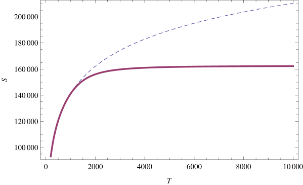
Figure 1: Plot of entropy of photon $S$ against temperature $T$ for both in the SR theory and DSR model; the dashed line corresponds to the SR theory result and the thick line represents the corresponding quantity in DSR. We have used the Planck units and the corresponding parameters take the following values $\kappa=10000$, $k_{\rm B}=1$, $N=10000$, $V=0.01$, $h=1$ in this plot. With this scale, $T=10000$ represents the Planck temperature.

In Fig. 1, we have plotted entropy against temperature for both the case of DSR and usual SR theory. It is clearly observable from the plot that the entropy grows at a much slower rate in case of DSR than in the SR theory and as temperature increases, the entropy in DSR model deviates more from the entropy in the SR theory. This result matches with our earlier expectation considering the underlying symmetry of the theory that the entropy in the DSR model should be less than the entropy in SR theory. As $T=10000$ is the Planck temperature, from the above plot one can see that the entropy saturates well before reaching the Planck scale (nearly around $T=2000$). However, this saturation temperature is still very much high to experimentally observe these DSR effects.

It is well known that the total number of microstates available to a system is a direct measure of the entropy for that system. Therefore our result merely reflects the fact that due to the existence of an energy upper bound $\kappa$ in the DSR model, the number of microstates gradually saturates to some finite value.

We expect modification in the expression of the internal energy $U$ for photon gas in the DSR model as the expression of entropy is modified and internal energy is related to the entropy as follows: $U=F+TS$. In the usual SR scenario, the explicit expression for internal energy is given by $U=3Nk_{\rm B}T$. But in the DSR scenario we considered, the expression for internal energy ($\tilde{U}$) of photon gas is the following

$$\tilde{U}=Nk_{\rm B}T\left[3-\frac{\kappa^{3}e^{-\frac{\kappa}{k_{\rm B}T}}}{2k_{\rm B}^{3}T^{3}-e^{-\frac{\kappa}{k_{\rm B}T}}\big{(}2k_{\rm B}^{3}T^{3}+2\kappa k_{\rm B}^{2}T^{2}+\kappa^{2}k_{\rm B}T\big{)}}\right].$$ (4.10)

It is easy to see from the expression of internal energy (4.10) that we get back the usual SR theory expression in the limit $\kappa\rightarrow\infty$. As in the case of entropy, here also we plot internal energy against temperature for both the SR and DSR case.

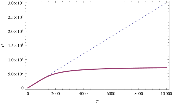
Figure 2: Plot of internal energy of photon against temperature for both in the SR theory and DSR scenario; the dashed line corresponds to the SR theory result and the thick line represents the quantity in the DSR model. We used the Planck units and the corresponding parameters take the following values $\kappa=10000$, $k_{\rm B}=1$, $N=10000$, $V=0.01$, $h=1$ in this plot. With this scale, $T=10000$ represents the Planck temperature.

In Fig. 2, we plotted internal energy of photon gas against its temperature for both the case of DSR model and SR theory. One can easily see from the plot that the value of internal energy (for a particular temperature) in the DSR model (4.10) is always less than its value (for the same temperature) in the SR theory. Since the internal energy $U$ of photon gas becomes saturated after a certain temperature in case of the DSR model, it is tempting to point out that probably our results are moving towards the right direction related to the “soccer ball problem” that plagues multi-particle description in the framework of DSR [43, 45].

In the next two sections, we discuss GUP effects for different types of scenarios.

5 Covariant formulation of GUP Lagrangian

Operatorial forms of noncommutative (NC) phase space structures has the generic form

$$\{x_{i},p_{j}\}=\delta_{ij}\big{(}1+f_{1}\big{(}{\mathbf{p}}^{2}\big{)}\big{)}+f_{2}\big{(}{\mathbf{p}}^{2}\big{)}p_{i}p_{j},$$

$$\{x_{i},x_{j}\}=f_{ij}({\mathbf{p}}),\qquad\{p_{i},p_{j}\}=g_{ij}({\mathbf{p}}),\qquad i=1,2,3.$$ (5.1)

Interestingly, potential application of (5.1) can generate generalized uncertainty principle (GUP) which is compatible with string theory expectation [4, 30, 55, 56, 73] that there exist a minimum length scale or a maximum momentum in nature. Such a length scale is defined to be of the order of ${\sqrt{\beta}}$, where $\beta$ can be treated as a small parameter. The corresponding models of GUP have been proposed in a non-covariant framework, by Kempf [48] (a two-parameter model, with $\beta$ and $\beta^{\prime}$)

$$\{x_{i},p_{j}\}=\delta_{ij}\big{(}1+\beta{\mathbf{p}}^{2}\big{)}+\beta^{\prime}p_{i}p_{j},$$

$$\{x_{i},x_{j}\}=(\beta^{\prime}-2\beta)(x_{i}p_{j}-x_{j}p_{i}),\qquad\{p_{i},p_{j}\}=0$$ (5.2)

by Kempf, Mangano and Mann [50]

$$\{x_{i},p_{j}\}=\delta_{ij}\big{(}1+\beta{\mathbf{p}}^{2}\big{)},\qquad\{x_{i},x_{j}\}=-2\beta(x_{i}p_{j}-x_{j}p_{i}),\qquad\{p_{i},p_{j}\}=0,$$ (5.3)

and also by Kempf and Mangano [49]

$$\{x_{i},p_{j}\}=\frac{\beta{\mathbf{p}}^{2}\delta_{ij}}{\sqrt{\big{(}1+2\beta{\mathbf{p}}^{2}\big{)}}-1}+\beta p_{i}p_{j},\qquad\{x_{i},x_{j}\}=0,\qquad\{p_{i},p_{j}\}=0.$$ (5.4)

The first NC algebra proposed by Snyder [71] has the same structure that of (5.3). In fact (5.2) [48] and (5.3) [50] can be reduced to the Snyder NC form [71] as discussed in [70]. Here we restrict ourselves to the classical counterpart of the commutator algebra (5.4) [49] since it is structurally the simplest as the coordinates and momenta commute among themselves respectively. But the results derived here are applied to quantum commutators as well.

We will consider a relativistically covariant generalization of the algebra (5.4). Starting with this algebra, firstly we study a generalized point particle Lagrangian [69] with a non-canonical symplectic structure that is equivalent to (5.4). Latter on by introducing electrodynamic interaction term in Lagrangian we further study point particle dynamics [69]. Now from a physical point of view this type of an intuitive particle picture is very useful and appealing since we can see how it differs from the conventional relativistic point particle. Also this particle model can act as a precursor to field theories in such non-canonical space. Similar point particle symplectic formalisms have been adopted in other forms of operatorial NC algebras, such as $\kappa$-Minkowski algebra [13, 14, 26, 32, 33, 34, 37, 63, 68], relevant in doubly special relativity framework [5, 6, 7, 8] or very special relativity algebra [21, 36], proposed in [19]. However, the crucial thing for one is to realize that the Jacobi identity is maintained by the linearized algebra [70]

$$\{X_{\mu},P_{\nu}\}=\delta_{\mu\nu}\big{(}1+\beta P^{2}\big{)}+2\beta P_{\mu}P_{\nu},\qquad\{P_{\mu},P_{\nu}\}=\{X_{\mu},X_{\nu}\}=0$$

only to $\cal{O}(\beta)$. If we consider $J(X_{\mu},X_{\nu},P_{\lambda})$ to be of the operatorial form

$$J(X_{\mu},X_{\nu},P_{\lambda})=\{X_{\mu},\{X_{\nu},P_{\lambda}\}\}+\{P_{\lambda},\{X_{\mu},X_{\nu}\}\}+\{X_{\nu},\{P_{\lambda},X_{\mu}\}\},$$

then we get

$$J(X_{\mu},X_{\nu},P_{\lambda})=4\beta^{2}P^{2}(\delta_{\nu\lambda}P_{\mu}-\delta_{\mu\lambda}P_{\nu}).$$

But exact validity of Jacobi identity is quite imperative for the phase space algebra. Furthermore, due to this violation of Jacobi, there can not be any point particle interpretation of this NC symplectic structure. This is due to the fact that the NC structures appear as Dirac brackets which always preserve Jacobi identity [27]. Therefore we will also construct deformed Poincaré generators that generate proper translations and rotations of the variables.

5.1 Covariantized point particle Lagrangian

We begin by positing covariantized form of the NC algebra proposed in [49] in $3+1$ dimensions, with a Minkowski metric $\eta_{\mu\nu}\equiv(1,-1,-1,-1)$

$$\{x_{\mu},p_{\nu}\}=-\frac{\beta p^{2}g_{\mu\nu}}{\sqrt{(1+2\beta p^{2})}-1}-\beta p_{\mu}p_{\nu}\equiv-\Lambda g_{\mu\nu}-\beta p_{\mu}p_{\nu},$$

$$\{x_{\mu},x_{\nu}\}=0,\qquad\{p_{\mu},p_{\nu}\}=0,$$ (5.5)

where $\Lambda=\frac{\beta p^{2}}{\sqrt{(1+2\beta p^{2})}-1}$. We would like to interpret the above relations (5.5) as Dirac brackets derived from a constrained symplectic structure. In some sense we are actually moving in the opposite direction of the conventional analysis where the computational steps are

$${\rm Lagrangian}~{}\rightarrow~{}{\rm constraints}~{}\rightarrow~{}{\rm Dirac~{}brackets}$$

or equivalently

$${\rm symplectic~{}structure}~{}\rightarrow~{}{\rm symplectic~{}matrix}~{}\rightarrow~{}{\rm symplectic~{}brackets}.$$

Interestingly the Dirac brackets and symplectic brackets turn out to be the same. In this case our path of analysis will be

$${\rm symplectic~{}brackets}~{}\rightarrow~{}{\rm symplectic~{}matrix}~{}\rightarrow~{}{\rm Lagrangian}.$$

Following this path, the symplectic matrix can be formed using (5.5) as

$$\Gamma_{ab}^{\mu\nu}=\left[\begin{matrix}0&-(\Lambda g^{\mu\nu}+\beta p^{\mu}p^{\nu})\\ (\Lambda g^{\mu\nu}+\beta p^{\mu}p^{\nu})&0\end{matrix}\right].$$

Inverse of this matrix provides commutators between the constraints as

$$\Gamma^{ab}_{\nu\lambda}=\left[\begin{matrix}0&\left(\dfrac{g_{\nu\lambda}}{\Lambda}-\dfrac{\beta p_{\nu}p_{\lambda}}{\Lambda^{2}{\sqrt{1+2\beta p^{2}}}}\right)\\ -\left(\dfrac{g_{\nu\lambda}}{\Lambda}-\dfrac{\beta p_{\nu}p_{\lambda}}{\Lambda^{2}{\sqrt{1+2\beta p^{2}}}}\right)&0\end{matrix}\right]\equiv\big{\{}\Phi^{a}_{\nu},\Phi^{a}_{\lambda}\big{\}}.$$ (5.6)

Indeed there is no unique way but from the constraint matrix one can make a judicious choice of the constraints and subsequently guess a form of the Lagrangian. We do not claim the Lagrangian derived in this way is unique, but one can easily check that the derived Lagrangian yields the same Dirac brackets that one posited at the beginning. Now it is convenient to work in the first order formalism where both $x_{\mu}$ and $p_{\mu}$ are treated as independent variables with the conjugate momenta, $\pi_{\mu}^{x}=\frac{\partial L}{\partial\dot{x^{\mu}}}$, $\pi_{\mu}^{p}=\frac{\partial L}{\partial\dot{p^{\mu}}}$ satisfying $\{x_{\mu},\pi_{\mu}^{x}\}=-g_{\mu\nu}$, $\{p_{\mu},\pi_{\mu}^{p}\}=-g_{\mu\nu}$. We obtain from (5.6) the following set of constraints

$$\Phi_{\mu}^{1}=\pi_{\mu}^{x}\approx 0,\qquad\Phi_{\mu}^{2}=\pi_{\mu}^{p}+\frac{x_{\mu}}{\Lambda}-\frac{\beta(xp)p_{\mu}}{\Lambda^{2}\sqrt{1+2\beta p^{2}}}\approx 0.$$

From this constraint structure we can finally write down the cherished form of the point particle Lagrangian in the first order formalism of $(x,p)$ as

$$L=-\frac{(x\dot{p})}{\Lambda}+\frac{\beta(xp)(p\dot{p})}{\Lambda^{2}\sqrt{1+2\beta p^{2}}}+\lambda\big{(}f(p^{2})-m^{2}\big{)},$$ (5.7)

where $\lambda$ is a Lagrange multiplier. This construction of the particle model Lagrangian is one of our major results [69]. We have included a mass-shell condition $f(p^{2})-m^{2}=0$ where $f(p^{2})$ denotes an arbitrary function that needs to fixed. The Lorentz generators get modified to

$$j_{\mu\nu}=\frac{1}{\Lambda}(x_{\mu}p_{\nu}-x_{\nu}p_{\mu}),$$

such that correct transformation of the degrees of freedom are reproduced

$$\{j_{\mu\nu},p_{\lambda}\}=g_{\mu\lambda}p_{\nu}-g_{\nu\lambda}p_{\mu},\qquad\{j_{\mu\nu},x_{\lambda}\}=g_{\mu\lambda}x_{\nu}-g_{\nu\lambda}x_{\mu}.$$

Interestingly this $j_{\mu\nu}$ obeys the correct Lorentz algebra

$$\{j_{\mu\nu},j_{\alpha\beta}\}=g_{\mu\alpha}j_{\nu\beta}-g_{\mu\beta}j_{\nu\alpha}-g_{\nu\beta}j_{\alpha\mu}+g_{\nu\alpha}j_{\beta\mu}.$$ (5.8)

Now since $\{j_{\mu\nu},p^{2}\}=0$, any function of $p^{2}$ is Lorentz invariant. But keeping translation invariance in mind, a more natural choice of $f(p^{2})$ would be $f(p^{2})\rightarrow\frac{p^{2}}{\Lambda^{2}}$ leading to a modified mass shell condition $\frac{p^{2}}{\Lambda^{2}}-m^{2}=0$. However this can be actually simplified to $p^{2}=M^{2}$, $M=m/\big{(}1-\frac{\beta m^{2}}{2}\big{)}$.

5.1.1 Approximations leading to other algebras

As we have explained at the beginning, approximating the full NC algebra (5.5) is not the proper way to derive an effective ${\cal O}(\beta)$ corrected dynamical system since, in particular with operatorial NC algebras, there is always a drawback that Jacobi identities might be violated. The correct way is to approximate the system at the level of the Lagrangian because then we are assured that the ${\cal O}(\beta)$ corrected NC brackets will also satisfy the Jacobi identities.

${\cal O}(\beta)$ results. To the first order approximation of $\beta$, the function $\Lambda$ becomes $\Lambda=1+\frac{1}{2}\beta p^{2}+{\cal O}(\beta^{2})$, using which the equation (5.7) provides the Lagrangian $L_{(1)}$ (without the mass-shell condition) as

$$L_{(1)}=-(x\dot{p})\left(1-\frac{1}{2}\beta p^{2}\right)+\beta(xp)(p\dot{p})+{\cal O}\big{(}\beta^{2}\big{)}.$$

The Dirac brackets turn out to be

$$\{x^{\mu},p^{\nu}\}=-\left[\frac{g_{\mu\nu}}{\left(1-\frac{\beta p^{2}}{2}\right)}+\frac{\beta p_{\mu}p_{\nu}}{\left(1-\frac{3\beta p^{2}}{2}\right)\left(1-\frac{\beta p^{2}}{2}\right)}\right],\qquad\{x^{\mu},x^{\nu}\}=\{p^{\mu},p^{\nu}\}=0.$$

Notice that the algebra is still structurally similar as the exact one and the Snyder form with non-zero $\{x_{\mu},x_{\nu}\}$ has not appeared. This agrees with previous results that the Snyder form is present only in ${\cal O}(\beta^{2})$ or when more than one $\beta$-like parameters are present [50, 70]. However, linearizing this algebra to ${\cal O}(\beta)$ is once again problematic as it clashes with the Jacobi identity. We will see that the Snyder form is necessary in the linearized system in order to exactly satisfy the Jacobi identity.

The combination $x_{\mu}$, $\big{(}1-\frac{\beta p^{2}}{2}\big{)}p_{\nu}$ constitutes a canonical pair with $\big{\{}x_{\mu},\big{(}1-\frac{\beta p^{2}}{2}\big{)}p_{\nu}\big{\}}=-g_{\mu\nu}$. The operator $j_{\mu\nu}=\big{(}1-\frac{\beta p^{2}}{2}\big{)}(x_{\mu}p_{\nu}-x_{\nu}p_{\mu})$ transforms $x_{\mu}$ and $p_{\mu}$ correctly and satisfies the correct Lorentz algebra (5.8).

${\cal O}(\beta^{2})$ results. With $\Lambda\approx 1+\frac{\beta p^{2}}{2}-\big{(}\frac{\beta p^{2}}{2}\big{)}^{2}$, the Lagrangian $L_{(2)}$ (without the mass-shell condition) becomes

$$L_{(2)}=-(x\dot{p})\left(1-\frac{\beta p^{2}}{2}+\left(\frac{\beta p^{2}}{2}\right)^{2}\right)+\beta(xp)(p\dot{p})\left(1-\frac{3\beta p^{2}}{2}\right).$$

The corresponding Dirac brackets are

$$\{x_{\mu},x_{\nu}\}=D(x_{\mu}p_{\nu}-x_{\nu}p_{\mu}),\qquad\{p_{\mu},p_{\nu}\}=0,$$

$$\{x_{\mu},p_{\nu}\}=-\frac{g_{\mu\nu}}{\Big{(}1-\frac{\beta p^{2}}{2}+\big{(}\frac{\beta p^{2}}{2}\big{)}^{2}\Big{)}}-Cp_{\mu}p_{\nu},$$

where

$$C=\frac{\beta\big{(}1-\frac{3\beta p^{2}}{2}\big{)}}{\big{(}1-\frac{3\beta p^{2}}{2}+\frac{7\beta^{2}p^{4}}{4}\big{)}\big{(}1-\frac{\beta p^{2}}{2}+\frac{\beta^{2}p^{4}}{4}\big{)}},\qquad D=\frac{C\beta p^{2}}{2\big{(}1-\frac{3\beta p^{2}}{2}\big{)}}.$$

We notice that the Snyder form has been recovered once ${\cal O}(\beta^{2})$ contributions are introduced. This GUP based Snyder algebra connection constitutes the other major result of our work [69]. It is possible to construct the deformed Poincaré generators but the expressions are quite involved and not very illuminating.

Two parameter $(\beta,\beta^{\prime})$ results. We now provide a considerably simpler Lagrangian with two parameters $\beta$ and $\beta^{\prime}$ that can induce the Snyder algebra. Note that ab initio it would have been hard to guess this result as well as the explicit expressions for the algebra but in our constraint framework this is quite straightforward. From the constraint analysis that generates the Dirac brackets it is clear that we need a non-vanishing $\{\phi_{2}^{\mu},\phi_{2}^{\nu}\}$ to reproduce a non-vanishing $\{x^{\mu},x^{\nu}\}$ bracket. Thus the two non-canonical terms in $L_{(1)}$ must have different $\beta$-factors to produce the desired effect. Hence we consider the Lagrangian $L_{(\beta,\beta^{\prime})}$ (without the mass-shell condition)

$$L_{(\beta,\beta^{\prime})}=-(x\dot{p})\left(1-\frac{\beta p^{2}}{2}\right)+\beta^{\prime}(xp)(p\dot{p}).$$

The Dirac brackets are obtained as

$$\{x_{\mu},x_{\nu}\}=D\frac{(\beta-\beta^{\prime})}{\beta^{\prime}}(x_{\mu}p_{\nu}-x_{\nu}p_{\mu}),\qquad\{p_{\mu},p_{\nu}\}=0,$$

$$\{x_{\mu},p_{\nu}\}=-\frac{g_{\mu\nu}}{\left(1-\frac{\beta p^{2}}{2}\right)}-Dp_{\mu}p_{\nu},$$

where $D=\frac{\beta^{\prime}}{\big{(}1-\frac{\beta p^{2}}{2}-\beta^{\prime}p^{2}\big{)}\big{(}1-\frac{\beta p^{2}}{2}\big{)}}$. Clearly for $\beta=\beta^{\prime}\rightarrow\{x_{\mu},x_{\nu}\}=0$, thus leaving a GUP like algebra. We have not shown the deformed Poincaré generators which are quite complicated.

5.2 Particle in external electromagnetic field

We introduce minimally coupled $U(1)$ gauge interaction to the free GUP particle Lagrangian (5.7)

$$L=-\frac{(x\dot{p})}{\Lambda}+\frac{\beta(xp)(p\dot{p})}{\Lambda^{2}\sqrt{1+2\beta p^{2}}}+\lambda\big{(}f\big{(}p^{2}\big{)}-m^{2}\big{)}+e(A\dot{x}).$$

Since the symplectic structure changes here, so we need to compute the new Dirac algebra though the procedure remains the same. Therefore in this case the Dirac brackets modified by the $U(1)$ interaction are given by

$$\{x_{\alpha},x_{\gamma}\}^{*}=0,\qquad\{x_{\alpha},p_{\gamma}\}^{*}=-(\Lambda g_{\alpha\gamma}+\beta p_{\alpha}p_{\gamma}),$$

$$\{p_{\alpha},p_{\gamma}\}^{*}=-e\Lambda(\Lambda F_{\alpha\gamma}+\beta p_{a}(F_{\alpha a}p_{\gamma}-F_{\gamma a}p_{\alpha})).$$ (5.9)

It is convenient to consider the relativistic Hamiltonian of the form

$$H=\frac{p^{2}}{m}-\sqrt{p^{2}}.$$ (5.10)

Using the Dirac brackets (5.9) and the Hamiltonian (5.10), the Hamilton’s equations of motion are obtained as,

$$\dot{x}_{\alpha}=\left\{x_{\alpha},\frac{p_{\gamma}p_{\gamma}}{m}-\sqrt{p_{\gamma}p_{\gamma}}\right\}^{*}=-\frac{1}{m}\Lambda^{2}\sqrt{1+2\beta p^{2}}p_{\alpha},$$

$$\dot{p}_{\alpha}=\left\{p_{\alpha},\frac{p_{\gamma}p_{\gamma}}{m}-\sqrt{p_{\gamma}p_{\gamma}}\right\}^{*}=-\frac{e}{m}\Lambda^{2}\sqrt{1+2\beta p^{2}}p_{\gamma}F_{\alpha\gamma}.$$ (5.11)

Keeping only ${\cal O}(e)$ terms we can eliminate $p$, to get the modified Newton’s law

$$\ddot{x}_{\alpha}=-\frac{e}{m}\Lambda^{2}\sqrt{1+2\beta p^{2}}\dot{x}_{\gamma}F_{\alpha\gamma}=-\frac{e}{m}\Lambda^{2}\sqrt{1+2\beta m^{2}}\dot{x}_{\gamma}F_{\alpha\gamma}.$$ (5.12)

It is important to note that the dynamics in (5.11) and (5.12) is exact for the GUP parameter $\beta$ although it is to the first order of $e$. Hence the dynamics remains qualitatively unchanged with a renormalization of the charge. The ${\cal O}(\beta)$ equation of motion is given by

$$\ddot{x}_{\alpha}=-\frac{e}{m}\big{(}1+2\beta m^{2}\big{)}\dot{x}_{\gamma}F_{\alpha\gamma}.$$

6 Path integral formulation for GUP Hamiltonian

The Heisenberg uncertainty principle (HUP) says that uncertainty in position decreases with increasing uncertainty in energy $(\Delta x\sim\frac{\hbar}{\Delta p})$. But HUP breaks down for energies close to Planck scale, at which point the Schwarzschild radius becomes comparable to Compton wavelength. Higher energies result in a further increase of the Schwarzschild radius, inducing the following relation: $\Delta x\approx l_{\rm P}^{2}\frac{\Delta p}{\hbar}$. Consistent with the above, the following form of GUP has been proposed, postulated to hold in all scales [50]

$$\Delta x_{i}\Delta p_{i}\geq\frac{\hbar}{2}\big{[}1+\beta\big{(}\Delta p^{2}+\langle p\rangle^{2}\big{)}+2\beta\big{(}\Delta p_{i}^{2}+\langle p_{i}\rangle^{2}\big{)}\big{]},\qquad i=1,2,3,$$ (6.1)

where $[\beta]=({\rm momentum})^{-2}$ and we will assume that $\beta\approx 1/(M_{\rm P}c)^{2}=l_{\rm P}^{2}/2\hbar^{2}$, $M_{\rm P}=$ Planck mass, and $M_{\rm P}c^{2}=$ Planck energy $\approx 10^{19}$ GeV. In one dimension the above inequality takes the form

$$\Delta x\Delta p\geq\frac{\hbar}{2}\left[1+3\beta(\Delta p^{2}+\langle p\rangle^{2})\right]$$ (6.2)

from which we have

$$\Delta p\leq\frac{\Delta x}{3\beta\hbar}+\sqrt{\left(\frac{\Delta x}{3\beta\hbar}\right)^{2}-\frac{1+3\beta\langle p\rangle^{2}}{3\beta}}.$$ (6.3)

Since $\Delta p$ is real quantity, we have

$$\left(\frac{\Delta x}{3\beta\hbar}\right)^{2}\geq\frac{1+3\beta\langle p\rangle^{2}}{3\beta}\ \Rightarrow\ \Delta x\geq\hbar\sqrt{3\beta}\sqrt{1+3\beta\langle p\rangle^{2}},$$ (6.4)

which gives the minimum bound for $\Delta x$ as

$$\Delta x_{\min}=\hbar\sqrt{3\beta}.$$ (6.5)

Here one should notice from (6.4) that the condition $\langle p\rangle=0$ gives this minimum bound (6.5), which is consistent with the above inequality (6.3) and GUP relation (6.2). Now using relation (6.5) along with the condition $\langle p\rangle=0$ we get the maximum bound of $\Delta p$ as

$$\Delta p_{\max}=\frac{1}{\sqrt{3\beta}}.$$ (6.6)

It can be shown [50] that the inequality (6.1) follows from the modified Heisenberg algebra

$$[x_{i},p_{j}]=i\hbar\big{(}\delta_{ij}+\beta\delta_{ij}p^{2}+2\beta p_{i}p_{j}\big{)}.$$ (6.7)

In this section, we use the notation $[\,,\,]$ instead of $\{\,,\,\}$ as used in the previous sections of this article to denote brackets since we are now dealing with quantum Lie algebraic structure. To satisfy the Jacobi identity, the above bracket (6.7) gives $[x_{i},x_{j}]=[p_{i},p_{j}]=0$, to first order in ${\cal O}(\beta)$ [48]. Now defining

$$x_{i}=x_{0i},\qquad p_{i}=p_{0i}\big{(}1+\beta p_{0}^{2}\big{)},$$ (6.8)

where $p_{0}^{2}=\sum\limits_{j=1}^{3}p_{0j}p_{0j}$ and $x_{0i}$, $p_{0j}$ satisfy the canonical commutation relations $[x_{0i},p_{0j}]=i\hbar\delta_{ij}$, one can easily show that the above commutation relation (6.7) is satisfied, to first order of $\beta$. Henceforth, we neglect terms of order $\beta^{2}$ and higher. The effects of this GUP (6.1) in Lamb shift and Landau levels have been studied in [24]. Also, formulation of coherent states for this GUP has been described in [35]. Here we successfully derive the kernel for this GUP model by Hamiltonian path integral formulation [31] and show that this GUP corrected kernel induces a maximum momentum bound in the theory [22].

Using (6.8), we start with the corresponding Hamiltonian of the form

$$H=\frac{p^{2}}{2m}+V(\vec{r}),$$

which can be written as

$$H=H_{0}+H_{1}+{\cal O}\big{(}\beta^{2}\big{)},$$ (6.9)

where

$$H_{0}=\frac{p_{0}^{2}}{2m}+V(\vec{r}),\qquad H_{1}=\frac{\beta}{m}p_{0}^{4}.$$

Thus, we see that any system with an well defined quantum (or even classical) Hamiltonian $H_{0}$, is perturbed by $H_{1}$, near the Planck scale. In other words, quantum gravity effects are in some sense universal. Now the modified Schrödinger equation corresponding to the above Hamiltonian (6.9) is given by

$$-\frac{\hbar^{2}}{2m}\frac{\partial^{2}}{\partial x^{2}}\psi(x,t)+\frac{\beta\hbar^{4}}{m}\frac{\partial^{4}}{\partial x^{4}}\psi(x,t)+V(x)\psi=i\hbar\frac{\partial}{\partial t}\psi(x,t).$$

In this article we show that path integral method [28] is applicable to this higher energy cases and we evaluate the free particle kernel for GUP corrected Hamiltonian (6.9). For this purpose, we shall briefly recall the notion of basic properties of kernel in Hamiltonian path integral formalism. The kernel in Hamiltonian path integral is given by [31]

$$K(x^{\prime\prime},x^{\prime})=\int\left[e^{\frac{i}{\hbar}\int(\vec{p}.\vec{\dot{x}}-H)dt}\right]\frac{dp_{1}}{2\pi\hbar}\frac{dp_{2}}{2\pi\hbar}\cdots\frac{dp_{N}}{2\pi\hbar}dx_{1}dx_{2}\cdots dx_{N-1}.$$ (6.10)

It has been shown in [31] that the above kernel (6.10) can be written in the form

$$K(x^{\prime\prime},x^{\prime},\Delta t)=\delta(\vec{x}^{\prime\prime}-\vec{x}^{\prime})-\frac{i\Delta t}{\hbar}\left[-\frac{\hbar^{2}\nabla^{2}}{2m}\times\delta(\vec{x}^{\prime\prime}-\vec{x}^{\prime})+\bar{V}(x)\delta(\vec{x}^{\prime\prime}-\vec{x}^{\prime})\right]$$

from which one can easily obtain Schrödinger equation using the relation

$$\psi(x^{\prime\prime},t^{\prime\prime})=\int K(x^{\prime\prime},t^{\prime\prime};x^{\prime},t^{\prime})\psi(x^{\prime},t^{\prime})dx^{\prime}.$$ (6.11)

Since

$$\int\psi^{*}(x^{\prime\prime},t^{\prime\prime})\psi(x^{\prime\prime},t^{\prime\prime})dx^{\prime\prime}=\int\psi^{*}(x^{\prime},t^{\prime})\psi(x^{\prime},t^{\prime})dx^{\prime},$$

using the relation (6.11) we have

$$\iiint K^{*}(x^{\prime\prime},t^{\prime\prime};x^{\prime}_{1},t^{\prime})K(x^{\prime\prime},t^{\prime\prime};x^{\prime},t^{\prime})\psi^{*}(x^{\prime}_{1},t^{\prime})\psi(x^{\prime},t^{\prime})dx^{\prime\prime}dx^{\prime}_{1}dx^{\prime}=\int\psi^{*}(x^{\prime},t^{\prime})\psi(x^{\prime},t^{\prime})dx^{\prime},$$

which immediately implies the following relation

$$\iint K^{*}(x^{\prime\prime},t^{\prime\prime};x^{\prime}_{1},t^{\prime})K(x^{\prime\prime},t^{\prime\prime};x^{\prime},t^{\prime})\psi^{*}(x^{\prime}_{1},t^{\prime})dx^{\prime\prime}dx^{\prime}_{1}=\psi^{*}(x^{\prime},t^{\prime}).$$ (6.12)

Also, if $\psi(x,t)$ is the solution of the Schrödinger equation

$$-\frac{\hbar^{2}}{2m}\nabla^{2}\psi(x,t)+V(x)\psi(x,t)=i\hbar\frac{\partial\psi(x,t)}{\partial t},$$

then the kernel also satisfy Schrödinger equation at the end point $x=x^{\prime\prime}$, i.e.

$$-\frac{\hbar^{2}}{2m}\frac{\partial^{2}}{{\partial x^{\prime\prime}}^{2}}K(x^{\prime\prime},t^{\prime\prime};x^{\prime},t^{\prime})+V(x^{\prime\prime})K(x^{\prime\prime},t^{\prime\prime};x^{\prime},t^{\prime})=i\hbar\frac{\partial}{\partial t^{\prime\prime}}K(x^{\prime\prime},t^{\prime\prime};x^{\prime},t^{\prime}).$$ (6.13)

Equation (6.11), (6.12) and (6.13) are the basic properties of the kernel $K(x,t)$.

6.1 Kernel for GUP corrected Hamiltonian

Path integral method [28] is applicable in all cases where the change of action, corresponding to the variation of path, is large enough compared to $\hbar$. As the above Hamiltonian (6.9) is associated with higher energy, so a small variation on paths other than the path of least action make enormous change in phase for which cosine or sine will oscillate exceedingly rapidly between plus and minus value and cancel out their total contribution. So only the least action path will contribute in kernel. This is similar to the idea of path integral in quantum mechanics. We now therefore consider the Hamiltonian (6.9) in one dimension

$$H=\frac{p_{0}^{2}}{2m}+\frac{\beta}{m}p_{0}^{4}+V(x).$$

If we consider that the particle goes from $x^{\prime}$ to $x^{\prime\prime}$ during the short time interval $\Delta t$, then the infinitesimal kernel is of the form

$$K(x^{\prime\prime},t^{\prime}+\Delta t;x^{\prime},t^{\prime})=\int e^{\frac{i}{\hbar}\int_{t^{\prime}}^{t^{\prime}+\Delta t}\left(p_{0}.\dot{x}-\frac{p_{0}^{2}}{2m}-\frac{\beta}{m}p_{0}^{4}-V(x)\right)dt}\frac{dp_{0}}{2\pi\hbar}$$

$$\phantom{K(x^{\prime\prime},t^{\prime}+\Delta t;x^{\prime},t^{\prime})}=\int e^{\frac{i}{\hbar}p_{0}.(x^{\prime\prime}-x^{\prime})}e^{-\frac{i}{\hbar}\left[\frac{p_{0}^{2}\Delta t}{2m}+\frac{\beta\Delta t}{m}p_{0}^{4}+\Delta t\bar{V}(x)\right]}\frac{dp_{0}}{2\pi\hbar},$$ (6.14)

where $\bar{V}(x)$ is the average of $V(x)$ over the straight line connecting $x^{\prime\prime}$ and $x^{\prime}$. Expanding the second exponential function in (6.14) and neglecting the second and higher order terms of $\Delta t$, we have

$$K(x^{\prime\prime},t^{\prime}+\Delta t;x^{\prime},t^{\prime})=\delta(x^{\prime\prime}-x^{\prime})$$

$$\qquad{}{}-\frac{i\Delta t}{\hbar}\left[-\frac{\hbar^{2}}{2m}\frac{\partial^{2}}{{\partial x^{\prime\prime}}^{2}}\delta(x^{\prime\prime}-x^{\prime})+\frac{\beta\hbar^{4}}{m}\frac{\partial^{4}}{{\partial x^{\prime\prime}}^{4}}\delta(x^{\prime\prime}-x^{\prime})+\bar{V}(x)\delta(x^{\prime\prime}-x^{\prime})\right].$$ (6.15)

It is interesting to note that the kernel (6.15) boils down to the same form as in [31] in the limit $\beta\to 0$. But it is very difficult to deal with above form of kernel (6.15) as it contains derivative of delta function. Therefore we are going to derive the delta-independent equivalent form of kernel. For this we consider the kernel for free particle

$$K(x^{\prime\prime},t^{\prime}+\Delta t;x^{\prime},t^{\prime})=\int e^{\frac{i}{\hbar}\int_{t^{\prime}}^{t^{\prime}+\Delta t}\left(p_{0}.\dot{x}-\frac{p_{0}^{2}}{2m}-\frac{\beta}{m}p_{0}^{4}\right)dt}\frac{dp_{0}}{2\pi\hbar},$$ (6.16)

for short time interval $\Delta t$. Now expanding the exponential series of the last term in (6.16) and neglecting the terms containing higher order of $\beta$ we have

$$K(x^{\prime\prime},t^{\prime}+\Delta t;x^{\prime},t^{\prime})=\int e^{-\frac{i\Delta t}{2m\hbar}\left(p_{0}-\frac{(x^{\prime\prime}-x^{\prime})m}{\Delta t}\right)^{2}+\frac{im(x^{\prime\prime}-x^{\prime})^{2}}{2\hbar\Delta t}}\left(1-\frac{i\beta\Delta tp_{0}^{4}}{\hbar m}\right)\frac{dp_{0}}{2\pi\hbar}.$$

After some calculation we get the kernel as

$$K(x^{\prime\prime},t^{\prime}+\Delta t;x^{\prime},t^{\prime})$$

$$\qquad=\sqrt{\frac{m}{2\pi i\hbar\Delta t}}\left[1+\frac{3\beta i\hbar m}{\Delta t}-\frac{6\beta m^{2}(x^{\prime\prime}-x^{\prime})^{2}}{{\Delta t}^{2}}-\frac{i\beta m^{3}(x^{\prime\prime}-x^{\prime})^{4}}{\hbar{\Delta t}^{3}}\right]e^{\frac{im(x^{\prime\prime}-x^{\prime})^{2}}{2\hbar\Delta t}}.$$ (6.17)

After a bit of lengthy algebra (please see [22] for details), the final form of the kernel becomes

$$K(x^{\prime\prime},t^{\prime\prime};x^{\prime},t^{\prime})=\sqrt{\frac{m}{2\pi i\hbar(t^{\prime\prime}-t^{\prime})}}$$

$$\hphantom{K(x^{\prime\prime},t^{\prime\prime};x^{\prime},t^{\prime})=}{}\times e^{\frac{im(x^{\prime\prime}-x^{\prime})^{2}}{2\hbar(t^{\prime\prime}-t^{\prime})}}\left[1+\frac{3\beta i\hbar m}{(t^{\prime\prime}-t^{\prime})}-\frac{6\beta m^{2}(x^{\prime\prime}-x^{\prime})^{2}}{(t^{\prime\prime}-t^{\prime})^{2}}-\frac{i\beta m^{3}(x^{\prime\prime}-x^{\prime})^{4}}{\hbar(t^{\prime\prime}-t^{\prime})^{3}}\right],\!\!\!$$ (6.18)

where $t^{\prime\prime}-t^{\prime}=N\Delta t$. This kernel (6.18) is exactly of the same form as the kernel for the infinitesimal interval (6.17). It can be shown that the above kernel (6.18) satisfies the modified schrodinger equation

$$-\frac{\hbar^{2}}{2m}\frac{\partial^{2}}{\partial x^{2}}\psi(x,t)+\frac{\beta\hbar^{4}}{m}\frac{\partial^{4}}{\partial x^{4}}\psi(x,t)=i\hbar\frac{\partial}{\partial t}\psi(x,t),$$ (6.19)

at the point $x=x^{\prime\prime}$, $t=t^{\prime\prime}$. Now the solution of this Schrödinger equation (6.19) is given by [24]

$$\psi(x,t)=\Big{(}Ae^{ik(1-\beta\hbar^{2}k^{2})x-\frac{iEt}{\hbar}}$$

$$\phantom{\psi(x,t)=}{}+Be^{-ik(1-\beta\hbar^{2}k^{2})x-\frac{iEt}{\hbar}}+Ce^{\frac{x}{\sqrt{2\beta\hbar^{2}}}-\frac{iEt}{\hbar}}+De^{-\frac{x}{\sqrt{2\beta\hbar^{2}}}-\frac{iEt}{\hbar}}\Big{)}.$$ (6.20)

With this solution (6.20) in hand, we can show that the kernels (6.15) and (6.17) indeed propagates the wave function $\psi(x,t)$ from a point $(x^{\prime},t^{\prime})$ to the point $(x^{\prime\prime},t^{\prime\prime})$, for a chosen time interval $\Delta t=t^{\prime\prime}-t^{\prime}$, such that $\frac{\Delta t}{4\beta\hbar m}=D$ = a dimensionless quantity of ${\cal O}(\beta)$. Thus the following relation holds

$$\psi(x^{\prime\prime},t^{\prime\prime})=\int K(x^{\prime\prime},t^{\prime\prime};x^{\prime},t^{\prime})\psi(x^{\prime},t^{\prime})dx^{\prime}.$$

Therefore the free particle kernel satisfies the basic properties of a kernel, which we have stated earlier.

For usual free particle case, the probability that a particle arrives at the point $x^{\prime\prime}$ is proportional to the absolute square of the kernel $K(x^{\prime\prime},x^{\prime},t^{\prime\prime}-t^{\prime})$, i.e. for usual free-particle kernel the probability is given by

$$P(x^{\prime\prime})dx=\frac{m}{2\pi\hbar(t^{\prime\prime}-t^{\prime})}dx.$$

Now, for the GUP corrected kernel (6.18), the corresponding probability is given by

$$P(x^{\prime\prime})dx=K^{*}(x^{\prime\prime},x^{\prime},t^{\prime\prime}-t^{\prime})K(x^{\prime\prime},x^{\prime},t^{\prime\prime}-t^{\prime})dx$$

$$\phantom{P(x^{\prime\prime})dx}=\left(1-\frac{12\beta m^{2}(x^{\prime\prime}-x^{\prime})^{2}}{(t^{\prime\prime}-t^{\prime})^{2}}\right)\frac{m}{2\pi\hbar(t^{\prime\prime}-t^{\prime})}dx.$$ (6.21)

It is clearly observable that the term $\big{(}1-\frac{12\beta m^{2}(x^{\prime\prime}-x^{\prime})^{2}}{(t^{\prime\prime}-t^{\prime})^{2}}\big{)}$ in (6.21) is smaller than 1 as $\beta>0$. Thus we conclude that the probability value in this case is less than the corresponding value in the free particle case. Also, since probability is non-negative, this term $\big{(}1-\frac{12\beta m^{2}(x^{\prime\prime}-x^{\prime})^{2}}{(t^{\prime\prime}-t^{\prime})^{2}}\big{)}$ should also be non-negative. Thus we have the following relation

$$1-\frac{12\beta m^{2}(x^{\prime\prime}-x^{\prime})^{2}}{(t^{\prime\prime}-t^{\prime})^{2}}\geq 0,$$

which immediately implies the bound for momentum as

$$p\leq p_{\max}=\frac{1}{2\sqrt{3\beta}},$$ (6.22)

where $p=\frac{mx}{t}$. Thus, from (6.22) we see that GUP induces a momentum upper bound in the theory which is comparable to maximum momentum uncertainty (6.6) induced by GUP.

Using this procedure, one can also calculate the GUP kernel for higher order terms of $\beta$, i.e. terms up to ${\cal O}(\beta^{2})$ [22]. It is interesting to note that the maximum momentum bound for ${\cal O}(\beta^{2})$ case is less than that obtained in the previous ${\cal O}(\beta)$ case, though by a very small amount (please see [22] for details).

7 Summary and discussion

A particular framework for quantum gravity is the doubly special relativity (DSR) formalism, that introduces a new observer independent energy scale, considered to be of the order of the Planck energy. Presence of this energy scale naturally invokes noncommutative phase space structure. We study the effects of this energy upper bound in relativistic thermodynamics for the particular case of $\kappa$-Minkowski spacetime where $\kappa$ plays the role of energy upper bound. We have explicitly computed the expression for the energy-momentum tensor of an ideal fluid in DSR framework [20]. In deriving the result we exploited the scheme of treating DSR as a nonlinear representation of the Lorentz group in special relativity.

We have also studied the modifications in the thermodynamic properties of photon gas in this DSR scenario where we have an invariant energy scale [23]. We show both analytically and graphically that the density of states and the entropy in this DSR framework are less than the corresponding quantities in Einstein’s special relativity (SR) theory. We stress that the Lorentz symmetry is not broken in this model. But due do the presence of an invariant energy upper bound in this theory, microstates can avail energies only up to a finite cut-off whereas in SR theory, microstates can attain energies up to infinity. The internal energy is modified in case of the DSR model and as a consequence the expression for the specific heat is also modified.

Though highly non-trivial, one can similarly study the behaviour of an ideal gas or fermion gas in case of this DSR model. There might be some modifications in the Fermi energy level which in turn can modify the Chandrasekhar mass limit for the white dwarf stars. Thus astrophysical phenomena in DSR framework is another issue which remains to be addressed.

Further, as we have the expression for energy-momentum tensor, one can study the cosmological aspects of the DSR model using the Friedmann equations. But this requires idea about the geometry sector (precisely the metric $g_{\mu\nu}$ and hence Einstein tensor $G_{\mu\nu}$) which is still unknown in the context of the DSR model. This still remains another open issue to be further studied.

It is noteworthy to mention here that “bouncing” loop quantum cosmology theories (for example see [16] and references therein) entail some modifications to the geometry of spacetime which in turn effectively put a bound on the curvature avoiding the big bang singularity. However, for these “bouncing” models, the perturbation technique cannot be used as at the point of curvature saturation, the energy density of the cosmic fluid diverges. So it is unclear how to construct the matter part of the Einstein equation. One alternative to avoid the big bang singularity is the inflation theory where the perturbation method can also be applied. On the other hand, in our model, the energy density of the cosmic fluid saturates to the Planck energy which is a finite real quantity. Possibly a combination of the model considered in this paper along with the “bouncing” loop quantum cosmology can successfully describe a situation where big bang singularity can be avoided.

We also have considered generalized uncertainty principle (GUP) induced models [69]. We derived a covariant free particle Lagrangian in GUP and also studied GUP Lagrangian in presence of an external electromagnetic field. We show how the equations of motion are affected by the noncommutative parameter present in the theory.

GUP gives rise additional terms in quantum mechanical Hamiltonian like $\beta p^{4}$, where $\beta\sim\frac{1}{(M_{\rm P}c)^{2}}$ is the GUP parameter. This term plays important role at Planck energy level. Considering this term as a perturbation, we have shown that path integral method is applicable on this GUP corrected non-relativistic cases [22]. Here we have constructed the explicit form of the GUP kernel by applying Hamiltonian path integral method. The consistency properties of this kernel is then thoroughly verified. We have shown that the probability for finding a particle at a given point in case of the GUP model is less than the corresponding probability in the canonical free particle case. We have also shown that probabilistic interpretation of this kernel induces a momentum upper bound in the theory. And this upper bound changes slightly with $e^{-{\cal O}(\beta^{2})}$, if we consider higher order $\beta$ terms in the Hamiltonian. Following this Hamiltonian path integral approach one can construct kernels and study their properties for other systems like particle in a step potential, Hydrogen atom etc, which is our future goal.

References

- [1] Albrecht A., Magueijo J., A time varying speed of light as a solution to cosmological puzzles, Phys. Rev. D 59 (1999), 043516, 13 pages, astro-ph/9811018.
- [2] Alexander S., Magueijo J., Noncommutative geometry as a realization of varying speed of light cosmology, hep-th/0104093.
- [3] Ali A.F., Majumder B., Towards a cosmology with minimal length and maximal energy, arXiv:1402.5104.
- [4] Amati D., Ciafaloni M., Veneziano G., Can spacetime be probed below the string size?, Phys. Lett. B 216 (1989), 41–47.
- [5] Amelino-Camelia G., Testable scenario for relativity with minimum-length, Phys. Lett. B 510 (2001), 255–263, hep-th/0012238.
- [6] Amelino-Camelia G., Doubly-special relativity: first results and key open problems, Internat. J. Modern Phys. D 11 (2002), 1643–1669, gr-qc/0210063.
- [7] Amelino-Camelia G., Relativity: special treatment, Nature 418 (2002), 34–35, gr-qc/0207049.
- [8] Amelino-Camelia G., Quantum-spacetime phenomenology, Living Rev. Relativity 16 (2013), 8, 137 pages, arXiv:0806.0339.
- [9] Amelino-Camelia G., Freidel L., Kowalski-Glikman J., Smolin L., The principle of relative locality, Phys. Rev. D 84 (2011), 084010, 13 pages, arXiv:1101.0931.
- [10] Amelino-Camelia G., Freidel L., Kowalski-Glikman J., Smolin L., Relative locality and the soccer ball problem, Phys. Rev. D 84 (2011), 087702, 5 pages, arXiv:1104.2019.
- [11] Amelino-Camelia G., Piran T., Planck-scale deformation of Lorentz symmetry as a solution to the ultrahigh energy cosmic ray and the TeV-photon paradoxes, Phys. Rev. D 64 (2001), 036005, 12 pages, astro-ph/0008107.
- [12] Awad A., Ali A.F., Planck-scale corrections to Friedmann equation, Cent. Eur. J. Phys. 12 (2014), 245–255, arXiv:1403.5319.
- [13] Banerjee R., Kulkarni S., Samanta S., Deformed symmetry in Snyder space and relativistic particle dynamics, J. High Energy Phys. 2006 (2006), no. 5, 077, 22 pages, hep-th/0602151.
- [14] Banerjee R., Kumar K., Roychowdhury D., Symmetries of Snyder–de Sitter space and relativistic particle dynamics, J. High Energy Phys. 2011 (2011), no. 3, 060, 14 pages, arXiv:1101.2021.
- [15] Bertolami O., Zarro C.A.D., Towards a noncommutative astrophysics, Phys. Rev. D 81 (2010), 025005, 8 pages, arXiv:0908.4196.
- [16] Bojowald M., Quantum gravity effects on space-time, arXiv:1002.2618.
- [17] Bruno N.R., Amelino-Camelia G., Kowalski-Glikman J., Deformed boost transformations that saturate at the Planck scale, Phys. Lett. B 522 (2001), 133–138, hep-th/0107039.
- [18] Camacho A., Macías A., Thermodynamics of a photon gas and deformed dispersion relations, Gen. Relativity Gravitation 39 (2007), 1175–1183, gr-qc/0702150.
- [19] Cohen A.G., Glashow S.L., Very special relativity, Phys. Rev. Lett. 97 (2006), 021601, 3 pages, hep-ph/0601236.
- [20] Das S., Ghosh S., Roychowdhury D., Relativistic thermodynamics with an invariant energy scale, Phys. Rev. D 80 (2009), 125036, 6 pages, arXiv:0908.0413.
- [21] Das S., Ghosh S., Mignemi S., Non-commutative spacetime in very special relativity, Phys. Lett. A 375 (2011), 3237–3242, arXiv:1004.5356.
- [22] Das S., Pramanik S., Path integral for nonrelativistic generalized uncertainty principle corrected Hamiltonian, Phys. Rev. D 86 (2012), 085004, 7 pages, arXiv:1205.3919.
- [23] Das S., Roychowdhury D., Thermodynamics of photon gas with an invariant energy scale, Phys. Rev. D 81 (2010), 085039, 7 pages, arXiv:1002.0192.
- [24] Das S., Vagenas E.C., Universality of quantum gravity corrections, Phys. Rev. Lett. 101 (2008), 221301, 4 pages, arXiv:0810.5333.
- [25] Daszkiewicz M., Lukierski J., Woronowicz M., Towards quantum noncommutative -deformed field theory, Phys. Rev. D 77 (2008), 105007, 10 pages, arXiv:0708.1561.
- [26] Deriglazov A.A., Poincaré covariant mechanics on noncommutative space, J. High Energy Phys. 2003 (2003), no. 3, 021, 9 pages, hep-th/0211105.
- [27] Dirac P.A.M., Lectures on quantum mechanics, Belfer Graduate School of Science Monographs Series, Vol. 2, Belfer Graduate School of Science, New York, 1967.
- [28] Feynman R.P., Hibbs A.R., Quantum mechanics and path integral, McGraw-Hill, New York, 1965.
- [29] Gangopadhyay S., Dutta A., Saha A., Generalized uncertainty principle and black hole thermodynamics, Gen. Relativity Gravitation 46 (2014), 1661, 10 pages, arXiv:1307.7045.
- [30] Garay L.J., Quantum gravity and minimum length, Internat. J. Modern Phys. A 10 (1995), 145–166, gr-qc/9403008.
- [31] Garrod C., Hamiltonian path-integral methods, Rev. Modern Phys. 38 (1966), 483–494.
- [32] Ghosh S., DSR relativistic particle in a Lagrangian formulation and non-commutative spacetime: a gauge independent analysis, Phys. Lett. B 648 (2007), 262–265, hep-th/0602009.
- [33] Ghosh S., Pal P., -Minkowski spacetime through exotic “oscillator”, Phys. Lett. B 618 (2005), 243–251, hep-th/0502192.
- [34] Ghosh S., Pal P., Deformed special relativity and deformed symmetries in a canonical framework, Phys. Rev. D 75 (2007), 105021, 11 pages, hep-th/0702159.
- [35] Ghosh S., Roy P., Stringy coherent states inspired by generalized uncertainty principle, Phys. Lett. B 711 (2012), 423–427, arXiv:1110.5136.
- [36] Gibbons G.W., Gomis J., Pope C.N., General very special relativity is Finsler geometry, Phys. Rev. D 76 (2007), 081701, 5 pages, arXiv:0707.2174.
- [37] Girelli F., Konopka T., Kowalski-Glikman J., Livine E.R., Free particle in deformed special relativity, Phys. Rev. D 73 (2006), 045009, 14 pages, hep-th/0512107.
- [38] Gradshteyn I.S., Ryzhik I.M., Table of integrals, series, and products, Academic Press, New York – London, 1965.
- [39] Granik A., Maguejo–Smolin transformation as a consequence of a specific definition of mass, velocity, and the upper limit on energy, hep-th/0207113.
- [40] Greiner W., Stocker N., Thermodynamics and statistical mechanics, Springer-Verlag, New York, 1995.
- [41] Hanson A.J., Regge T., Teitelboim C., Constrained Hamiltonian system, Accademia Nazionale Dei Lincei, Roma, 1976.
- [42] Hossenfelder S., A note on theories with a minimal length, Classical Quantum Gravity 23 (2006), 1815–1821, hep-th/0510245.
- [43] Hossenfelder S., Multiparticle states in deformed special relativity, Phys. Rev. D 75 (2007), 105005, 8 pages, hep-th/0702016.
- [44] Hossenfelder S., Minimal length scale scenarios for quantum gravity, Living Rev. Relativity 16 (2013), 2, 90 pages, arXiv:1203.6191.
- [45] Hossenfelder S., The soccer-ball problem, SIGMA 10 (2014), 074, 8 pages, arXiv:1403.2080.
- [46] Hossenfelder S., Bleicher M., Hofmann S., Ruppert J., Scherer S., Stöcker H., Signatures in the Planck regime, Phys. Lett. B 575 (2003), 85–99, hep-th/0305262.
- [47] Judes S., Visser M., Conservation laws in “doubly special relativity”, Phys. Rev. D 68 (2003), 045001, 4 pages, gr-qc/0205067.
- [48] Kempf A., Non-pointlike particles in harmonic oscillators, J. Phys. A: Math. Gen. 30 (1997), 2093–2101, hep-th/9604045.
- [49] Kempf A., Mangano G., Minimal length uncertainty relation and ultraviolet regularisation, Phys. Rev. D 55 (1997), 7909–7920, hep-th/9612084.
- [50] Kempf A., Mangano G., Mann R.B., Hilbert space representation of the minimal length uncertainty relation, Phys. Rev. D 52 (1995), 1108–1118, hep-th/9412167.
- [51] Kowalski-Glikman J., Nowak S., Doubly special relativity theories as different bases of -Poincaré algebra, Phys. Lett. B 539 (2002), 126–132, hep-th/0203040.
- [52] Ling Y., Wu Q., The big bounce in rainbow universe, Phys. Lett. B 687 (2010), 103–109, arXiv:0811.2615.
- [53] Lukierski J., Nowicki A., Doubly special relativity versus -deformation of relativistic kinematics, Internat. J. Modern Phys. A 18 (2003), 7–18, hep-th/0203065.
- [54] Maggiore M., A generalized uncertainty principle in quantum gravity, Phys. Lett. B 304 (1993), 65–69, hep-th/9301067.
- [55] Maggiore M., The algebraic structure of the generalized uncertainty principle, Phys. Lett. B 319 (1993), 83–86, hep-th/9309034.
- [56] Maggiore M., Quantum groups, gravity, and the generalized uncertainty principle, Phys. Rev. D 49 (1994), 5182–5187, hep-th/9305163.
- [57] Magueijo J., New varying speed of light theories, Rep. Progr. Phys. 66 (2003), 2025–2068, astro-ph/0305457.
- [58] Magueijo J., Smolin L., Lorentz invariance with an invariant energy scale, Phys. Rev. Lett. 88 (2002), 190403, 4 pages, hep-th/0112090.
- [59] Magueijo J., Smolin L., Generalized Lorentz invariance with an invariant energy scale, Phys. Rev. D 67 (2003), 044017, 12 pages, gr-qc/0207085.
- [60] Magueijo J., Smolin L., Gravity’s rainbow, Classical Quantum Gravity 21 (2004), 1725–1736, gr-qc/0305055.
- [61] Majhi B.R., Vagenas E., Modified dispersion relation, photon’s velocity, and Unruh effect, Phys. Lett. B 725 (1993), 477–480, arXiv:1307.4195.
- [62] Mersini-Houghton L., Bastero-Gil M., Kanti P., Relic dark energy from transPlanckian regime, Phys. Rev. D 64 (2001), 043508, 9 pages, hep-ph/0101210.
- [63] Mignemi S., Transformations of coordinates and Hamiltonian formalism in deformed special relativity, Phys. Rev. D 68 (2003), 065029, 6 pages, gr-qc/0304029.
- [64] Mignemi S., Doubly special relativity and translation invariance, Phys. Lett. B 672 (2009), 186–189, arXiv:0808.1628.
- [65] Misner C.W., Thorne K.S., Wheeler J.A., Gravitation, W.H. Freeman and Co., San Francisco, Calif., 1973.
- [66] Moffat J.W., Superluminary universe: a Possible solution to the initial value problem in cosmology, Internat. J. Modern Phys. D 2 (1993), 351–366, gr-qc/9211020.
- [67] Pathria R.K., Statistical mechanics, Butterworth-Heinemann, Oxford, 1996.
- [68] Pinzul A., Stern A., Space-time noncommutativity from particle mechanics, Phys. Lett. B 593 (2004), 279–286, hep-th/0402220.
- [69] Pramanik S., Ghosh S., GUP-based and Snyder noncommutative algebras, relativistic particle models, deformed symmetries and interaction: a unified approach, Internat. J. Modern Phys. A 28 (2013), 1350131, 15 pages, arXiv:1301.4042.
- [70] Quesne C., Tkachuk V.M., Composite system in deformed space with minimal length, Phys. Rev. A 81 (2010), 012106, 8 pages, arXiv:0906.0050.
- [71] Snyder H.S., Quantized space-time, Phys. Rev. 71 (1947), 38–41.
- [72] Tawfik A., Magdy H., Farag Ali A., Effects of quantum gravity on the inflationary parameters and thermodynamics of the early universe, Gen. Relativity Gravitation 45 (2013), 1227–1246, arXiv:1208.5655.
- [73] Townsend P.K., Small-scale structure of spacetime as the origin of the gravitational constant, Phys. Rev. D 15 (1977), 2795–2801.
- [74] Veneziano G., A stringy nature needs just two constants, Europhys. Lett. 2 (1986), 199–204.
- [75] Weinberg S., Gravitation and cosmology: principles and applications of general theory of relativity, John Wiley & Sons, London, 1972.