DNA nanotechnology: understanding and optimisation through simulation

Abstract

DNA nanotechnology promises to provide controllable self-assembly on the nanoscale, allowing for the design of static structures, dynamic machines and computational architectures. In this article I review the state-of-the art of DNA nanotechnology, highlighting the need for a more detailed understanding of the key processes, both in terms of theoretical modelling and experimental characterisation. I then consider coarse-grained models of DNA, mesoscale descriptions that have the potential to provide great insight into the operation of DNA nanotechnology if they are well designed. In particular, I discuss a number of nanotechnological systems that have been studied with oxDNA, a recently developed coarse-grained model, highlighting the subtle interplay of kinetic, thermodynamic and mechanical factors that can determine behaviour. Finally, new results highlighting the importance of mechanical tension in the operation of a two-footed walker are presented, demonstrating that recovery from an unintended ‘overstepped’ configuration can be accelerated by three to four orders of magnitude by application of a moderate tension to the walker’s track. More generally, the walker illustrates the possibility of biasing strand-displacement processes to affect the overall rate.
Key words: DNA nanotechnology; self-assembly; molecular machines; non-equilibrium systems; coarse-grained modelling; simulation.
*Correspondence: t.ouldridge@imperial.ac.uk

I Introduction to DNA nanotechnology

I.1 The DNA molecule and its potential

Deoxyribonucleic acid (DNA) is a macromolecule with a backbone of covalently linked sugar and phosphate groups; attached to each sugar is a base, which can be adenine (A), guanine (G), cytosine (C) or thymine (T) Saenger1984 . DNA is often found as a double helix of antiparallel strands stabilised by hydrogen-bonding of complementary Watson-Crick base pairs (AT and CG) and stacking interactions between the planar bases. Double-stranded DNA (dsDNA) is stiff, with a persistence length of $\sim 150$ base pairs Hagerman1988 , whereas unpaired single strands (ssDNA) are far more flexible Mills1999 ; Murphy2004 .

DNA carries information through its sequence of bases - in biology, this information codes for proteins and their regulation. The specificity of Watson-Crick base-pairing means that both strands within a duplex carry identical information, facilitating replication. In 1982, Seeman speculated that the specificity of DNA hybridization could be harnessed to permit the design of artificial structures, proposing that certain sequences could self-assemble into crystals Seeman1982 .

I.2 DNA nanostructures

The Seeman group quickly constructed artificial nucleic acid junctions Kallenbach83 , but the first 3-dimensional crystal based purely on rationally designed Watson-Crick base pairs was not demonstrated until 2009 Zheng2009 (crystals involving non-canonical interactions were created in 2004 Paukstelis2004 ). In the intervening period, ribbons Yan2003 and 2D lattices Winfree98 ; Malo2005 were realised. Complex Archimedean tiling patterns Zhang2013 and ‘empty liquids’ Biffi2013 have recently been achieved through hybridization-driven DNA self-assembly.

As well as macroscopic phases, DNA can form structures of well-defined finite size. Early successes (cubes Chen91 and octahedra Zhang94 ) involved several discrete stages of assembly, but it was subsequently shown that polyhedra Goodman2005 ; Erben07 ; Andersen08 and then more complex structures Wei2012 ; Ke2012 could be made to form simply by cooling solutions of short ssDNA strands (oligonucleotides). An alternative approach, known as DNA ‘origami’ Rothemund06 , uses one long ‘scaffold’ strand that is shaped by shorter ‘staple’ strands into a complex structure. This technique can produce three dimensional objects Douglas09 ; Andersen09 and structures with curvature or twist Dietz2009 ; Han2011 . Some examples of DNA nanostructures are shown in Fig. 1 (a)-(c).

DNA does not have to be used in isolation – it can also be conjugated with other molecules or nanoparticles. Crystals of DNA-coated colloids have been constructed Park2008 , and small organic molecules have been used as vertices in structures held together by DNA Aldaye2007 ; Zimmermann08 .

I.3 Dynamic DNA devices

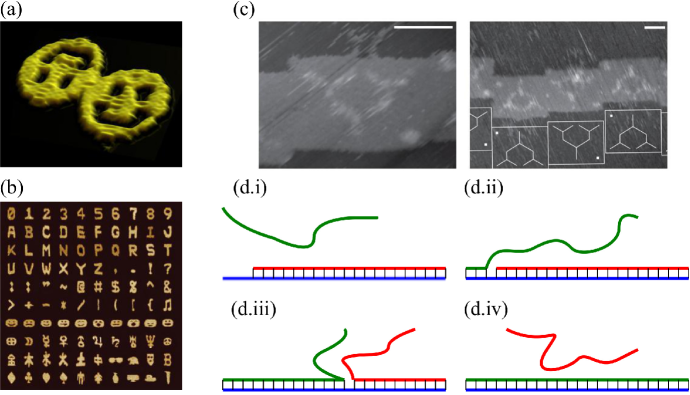
Figure 1: (a)-(c) Examples of DNA nanotechnology. (a) Atomic force microscopy (AFM) image of the original DNA ‘origami’ Rothemund06 , courtesy of P. W. K. Rothemund. (b) AFM of complex structures assembled from DNA ‘bricks’ Ke2012 , courtesy of P. Yin. (c) Tracks for a DNA-based motor on origami. Reprinted by permission from Macmillan Publishers Ltd: Nature Nanotechnology Wickham2012 , copyright 2012. (d) Basic displacement. (d.i) The initial state with incumbent (red) and substrate (blue) bound, and the invader (green) free in solution. (d.ii) The invader binds to the available toehold of the substrate. (d.iii) The invader competes with the incumbent for base pairs. (d.iv) The final state, in which the invader has completely displaced the incumbent.

DNA is not restricted to static nanostructures, but can be used to create dynamically active nanoscale objects. Toehold-mediated strand displacement (TMSD), illustrated in Fig. 1 (d), is used along with hybridisation to drive conformational changes in many such devices. TMSD involves the replacement of a strand (the incumbent) from a duplex with the substrate by an alternative strand (the invader) that is complementary to an additional toehold of the substrate. Initially, the invader can bind to the exposed toehold, as shown in Fig. 1 (d.ii) Yurke2003 ; Zhang_disp_2009 ; Srinivas2013 . The invader and incumbent can then compete for base-pairing, as illustrated in Fig. 1 (d.iii). If, eventually, the incumbent loses all of its base pairs, it will detach and displacement is complete (Fig. 1 (d.iv)). As well as being essential in dynamic nanotechnology, displacement may occur during the assembly of complex structures that initially form unintended bonds between the wrong strands.

The simplest devices are switches that respond to a change in experimental conditions. An iconic example are the ‘tweezers’ of Yurke et al. Yurke2000 , which can be closed and opened by sequential addition of ‘fuel’ strands (which bind to and closes the tweezers) and ‘antifuel’ strands (which displace the tweezers from the fuel, opening them). Switches can allow large structures to open, close or undergo topological rearrangement Yan2002 ; Goodman2008 ; Andersen09 ; Han2010 .

DNA ‘walkers’ couple the mechanical change generated by DNA reactions to motion along extended tracks, analogous to biological motors such as kinesin and myosin. The earliest designs used sequential strand addition to generate unidirectional motion along a series of binding sites (‘stators’) Sherman2004 ; Shin2004 . Solution conditions can also be modulated in different ways, for example through periodic exposure to light of different frequencies Liu2014 . Autonomous motors, which don’t rely on external control, must catalyse the release of free energy Bath2007 . To meet this requirement, designs often couple motion to the hydrolysis of a nucleic acid strand that is not part of the walker itself. Hydrolysis can be achieved either with Bath2005 ; Bath2009 ; Wickham2011 or without Tian2005 ; Lund2010 ; Cha2014 the involvement of an additional enzyme. An alternative is to catalyse DNA hybridisation itself Green2008 ; Omabegho2009 if the reactants are present as metastable self-bonded hairpins. Many walkers destroy the track behind them in the so-called ‘burnt bridges’ approach. The Turberfield group have also demonstrated the possibility of autonomous motion on a track that can be reused Green2008 ; Bath2009 . In the majority of cases, hybridisation and displacement are central to walker operation, sometimes in combination with additional enzymatic reactions. An alternative is to use four-way branch migration rather than displacement Venkataraman2007 ; Muscat2011 .

A third branch of active DNA nanotechnology is computation. In 1994 Adleman showed that a Hamiltonian path problem could be solved using DNA Adleman1994 . Subsequently, researchers have developed motifs for logical operation based on TMSD Seelig2006 , with the Winfree group having incorporated multiple gates into a decision-making ‘brain’ Qian2011 , and Chen et al. having developed a general architecture for control networks Chen2013 .

I.4 Applications of DNA nanotechnology

Many nanotechnological systems are elegant proofs of principle, rather than being directly useful. The potential of DNA nanotechnology, however, is obvious. Seeman’s original motivation was to use DNA crystals to conjugate proteins and facilitate crystallography; origami bundles and two-dimensional lattices have indeed been used to aid protein structure determination Berardi2011 ; Selmi2011 . Similarly, finite-sized nanostructures contain unique strands at well-defined locations. This allows nanostructures to function as nanoscale breadboards for biophysical systems – they have been used as backbones for plasmonic devices Kuzyk2012 and light-harvesting complexes Dutta2011 , to control Tseng2013 ; Minghui2013 and facilitate the study of Wilner2009 ; Fu2012 ; Fu2014 enzymatic reactions, and to provide tracks for DNA motors Wickham2012 ; Tomov2013 (as shown in Fig. 1 (c)). DNA nanostructures have also been designed to act as microscopic gene-detecting arrays Ke2008 ; Subramanian2011 . The freedom to design complex structures allows DNA to be used for other experimental components, including ‘handles’, ‘frames’ and ‘rulers’ for single-molecule manipulation Endo2012 ; Pfitzner2013 , and harnesses for arrays of motor proteins Derr2012 .

The therapeutic potential of DNA nanotechnology has long been recognised. Nanostructures can encapsulate molecules either covalently or non-covalently Douglas2012 ; Crawford2013 , with the aim of selectively releasing them at the surface of or inside specific cells. Alternatively, nanostructures can coordinate biomolecules to mimic pathogens, potentially triggering stronger immune responses Li2011 ; Schuller2012 ; Liu2012 and allowing the design of novel vaccines Liu2012 . DNA computation may also prove to be most valuable in medical applications, when its enormous parallel capacity and direct interaction with biomolecules will prove most advantageous. Towards this end, both the uptake of small nanostructures into cells Walsh2011 ; Li2011 ; Lee2012 and specific targeting of cancer cells by DNA-transported drugs Douglas2012 have been demonstrated. Large DNA nanostructures have been reported to be survive intact in cell lysate Mei2011 , and DNA-based devices and structures have been shown to be stable within C. elegans for hours or days, depending on the design Surana2013 . The Shih lab has also shown that lipid encapsulation of nanostructures can help to shield them from digestion by nucleases when this is an issue Perrault2014 and coating origami with virus capsid proteins has been shown to improve transfection into cells Mikkila2014 . Interacting “robots” have even been demonstrated to perform computations based on TMSD within a living organism Amir2014 .

Artificial walking devices could function as agents in molecular assembly lines, incorporating some degree of decision-making. Preliminary work has demonstrated that DNA hybridisation can accelerate and template reactions He2010 ; McKee2012 , that walkers can make decisions at junctions Muscat2011 ; Wickham2012 and that walkers can selectively pick up gold nanoparticle cargo Gu2010 .

I.5 Understanding and optimising DNA nanotechnology

If DNA nanotechnology is to be widely used, assembly processes and operation cycles must be understood and optimised. Simple self-assembling structures such as DNA tetrahedra form reliably when a solution of reactants is rapidly cooled Goodman2005 . Larger systems tend to be more complex, although recent work has shown that substantial structures can form surprisingly well if the temperature is carefully chosen Sobczak2012 ; Myhrvold2013 . It is not obvious, however, why assembly can be so successful given previous failures with large colloidal structures Reinhardt2014 . It is also not clear why origami assembly can occur over a very narrow temperature window Sobczak2012 , with significant hysteresis Sobczak2012 ; Arbona2013 . Improving yields of larger structures by choosing sequences to minimise unintended cross-interactions has shown surprisingly little promise thus far Wei2012 ; Ke2012 , but origami assembly is very sensitive to the staple layout Ke2012b ; Martin2012 ; Myhrvold2013 . Even if an object appears to form well, some strands might be absent, possibly compromising its usefulness and mechanical properties Chen2014 . Optimisation is even more important for dynamic nanotechnology, where relatively slow unintended reactions can compromise device operation Tomov2013 . For example, even if a walker has only a 5% chance of detaching from the track at each step, most will fail to take twenty steps. As it stands, motors are slow compared to natural analogs, and systematic approaches for improving their effectiveness or decision-making abilities are currently limited.

Recent experiments have probed specific systems relevant to nanotechnology in detail Zhang_disp_2009 ; Sobczak2012 ; Myhrvold2013 ; Ke2012b ; Martin2012 ; Tomov2013 ; Johnson-Buck2013 ; Tsukanov2013 ; Teichmann2014 . To interpret these results, generalise the resultant ideas and develop new principles, these systems must be modelled theoretically. To date, the main theoretical tool has been the nearest-neighbour model of DNA thermodynamics SantaLucia2004 , implemented in online tools such as NuPack Dirks2007 . The nearest-neighbour model functions at the level of secondary structure (i.e., lists of the base-pairing that is present in the system). The free energy of a given secondary structure can be estimated by summing contributions from each neighbouring ‘stack’ of base pairs, plus contributions from end effects and enclosed loops. Whilst the nearest-neighbour model is extremely useful, it has several limitations. Firstly, it is a thermodynamic model with discrete states and hence has no natural kinetics Srinivas2013 . Secondly, it does not explicitly represent DNA structure, and struggles to describe complex interconnections, loops and ‘pseudoknots’ Dirks2007 that often arise in nanotechnological systems. Finally, DNA mechanics is ignored, meaning that the effects of forces and torques cannot be directly understood.

Next, I will introduce coarse-grained models of DNA, mesoscale representations that can overcome the limitations of the nearest-neighbor description. I will focus on oxDNA, a model explicitly designed for DNA nanotechnology. I will outline the model, before discussing previous applications in understanding TMSD in a variety of contexts. Finally, new results will be presented on displacement involving a two-footed DNA walker Bath2009 , highlighting the possibility of accelerating displacement through mechanical strain.

II Coarse-grained modelling of DNA nanotechnology

Coarse-grained models provide a level of resolution between fully atomistic treatments and secondary-structure descriptions like the nearest-neighbour model. Atomistic treatments are generally too computationally expensive for nanotechnological applications, although some structural studies have been performed Oteri2011 ; Yoo2013 . Coarse-grained models represent individual nucleotides using a small number of interaction sites, which interact through effective potentials. If well parameterised, they can capture the known thermodynamic, structural and mechanical properties of DNA in a simple and naturally dynamical representation.

The choice of interactions determines the accuracy and applicability of the model. A ‘bottom-up’ approach is to fit interactions to reproduce correlation functions from more detailed atomistic simulations Becker2007 ; Becker2009 ; Lankas2009 ; Sayar2009 ; Savelyev2010 ; Dans2010 ; Morriss-Andrews2010 ; Kikot2011 ; Savin2011 ; Gonzalez2013 ; He2013 ; Kovaleva2014 ; Maffeo2014 ; Korolev2014 ; Naome2014 , or data from experimentally determined structures Olson1998 ; Becker2009 ; Trovato2008 ; He2013 This procedure can be very effective, but it has limitations. Firstly, the resultant model is very dependent on the source data, which are usually primarily drawn from duplex DNA, whereas nanotechnological systems involve ssDNA and hybridisation transitions (one exception has focused specifically on ssDNA only Maffeo2014 ). Even if a wider variety of systems were to be used for parameterisation, it is not clear whether current atomistic representations accurately describe isolated ssDNA and the hybridisation transition. Secondly, one cannot retain all features of a system when coarse-graining; ‘representability problems’ arise Johnson2007 . For a given set of coarse-grained degrees of freedom, the optimal potential for correlation functions will likely be distinct from that for thermodynamics. Related issues are relevant to potentials derived from ab initio calculations Hsu2012 .

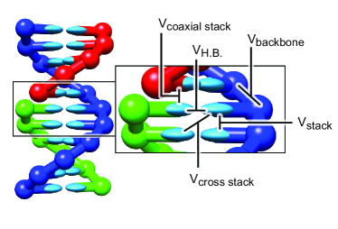
Figure 2: Illustration of the duplex structure and stabilising interactions with the oxDNA model. Spheres represent the backbone sites, and ellipsoids represent bases. Strands are coloured according to their identity. Coaxial stacking acts like a nearest-neighbour stacking interaction between bases that are not consecutive on the same strand. Excluded volume interactions (not illustrated here) also exist between all backbone and base sites. Reprinted with permission from T.E. Ouldridge, et al., Optimizing DNA nanotechnology through coarse-grained modelling: A two-footed DNA walker, ACS Nano 7, 2479. Copyright (2013) American Chemical Society.

Representability problems highlight the fact that coarse-grained models cannot be perfect, and hence should be designed with their purpose in mind. For nanotechnological systems, models must capture ssDNA, dsDNA and their interconversion. To date, this has been most successfully done with ‘top-down’ approaches Drukker2001 ; Sales-Pardo2005 ; Starr2006 ; Tito2010 ; Knotts2007 ; Sambriski2009_BiophysJ ; Hinckley2013 ; Svaneborg2012 ; Kenward2009 ; Linak2012 ; Araque2011 ; Niewieczerzal2009 ; Arbona2012b ; Edens2012 ; Dasanna2013 ; Cragnolini2013 ; Doi2010 ; Mielke2005 ; Knorowski2011 . Here, physically-motivated interactions such as hydrogen-bonding and stacking are included and parameterised to reproduce overall thermodynamic, mechanical and structural properties of DNA. In this article I focus on oxDNA Ouldridge2011 ; Ouldridge_thesis ; Sulc2012 , an attempt to incorporate thermodynamics as parameterised by the nearest-neighbour model into a description with continuous degrees of freedom that captures structural and mechanical properties of DNA. Due to the emphasis placed on capturing the duplex formation transition in the development of oxDNA, it has been used to study nanotechnological systems more extensively than other models. However, duplex and hairpin formation transitions have been systematically investigated by a number of groups Sales-Pardo2005 ; Starr2006 ; Tito2010 ; Allen2011 ; Sambriski2009_BiophysJ ; Prytkova2010 ; Hoefert2011 ; Schmitt2013 ; Hinckley2013 ; Linak2012 ; Edens2012 ; Cragnolini2013 ; Hinckley2014 , nanostructure conformation has been studied by Bombelli et al. and Arbona et al. Bombelli2008 ; Arbona2012b , and nanostructure assembly Arbona2012 ; Svaneborg2012b ; Ouldridge2009 and displacement Svaneborg2012c have been demonstrated with much simple models of DNA. Large-scale asssembly of DNA-coated objects has also been achieved with some simpler coarse-grained models Starr2006 ; Knorowski2011 ; Li2012 . It is worth noting that similar top-down Hyeon2005 ; Cao2006 ; Jost2010 ; Ding2008 ; Pasquali2010 ; Dickson2011 ; Cragnolini2013 ; Denesyuk2013 and bottom-up Jonikas2009 ; Das2009 ; Paliy2010 ; Xia2013 models exist for RNA.

II.0.1 oxDNA

oxDNA treats each nucleotide as a 3-dimensional rigid body. The potential energy of a configuration is given by

$$V=\sum_{\left\langle ij\right\rangle}\left(V_{\rm{b.b.}}+V_{\rm{stack}}+V^{{}^{\prime}}_{\rm{exc}}\right)+$$

$$\sum_{i,j\notin{\left\langle ij\right\rangle}}\left(V_{\rm HB}+V_{\rm{cr.st.}}+V_{\rm{exc}}+V_{\rm{cx.st.}}\right).$$ (1)

Here the first sum runs over all consecutive pairs of nucleotides on a strand, and the second sum over all remaining pairs. The interactions represent hydrogen bonding ($V_{\rm HB}$), cross stacking ($V_{\rm{cr.st.}}$), coaxial stacking ($V_{\rm{cx.st.}}$), nearest-neighbour stacking ($V_{\rm{stack}}$), excluded volume ($V_{\rm{exc}}$ or $V^{{}^{\prime}}_{\rm{exc}}$) and backbone chain connectivity ($V_{\rm{b.b.}}$). These interactions are shown schematically in Fig. 2, and are discussed in detail elsewhere Ouldridge2011 ; Ouldridge_thesis ; Sulc2012 . Importantly, attractive interactions depend explicitly on the relative orientations of nucleotides, allowing the anisotropic nature of bases to play a role.

Hydrogen-bonding and stacking interactions drive the formation of duplexes with helical structure from single strands that are relatively more disordered. oxDNA reproduces the thermodynamic, mechanical and structural changes associated with this transition, under high salt conditions. In particular, oxDNA provides a good representation of duplex melting temperatures, melting transitions widths, self-complementary hairpin stability, duplex elastic moduli and the short persistence length of single strands (details are provided in Refs. Ouldridge2011 ; Ouldridge_thesis ; Sulc2012 ). Our group uses the “Virtual Move Monte Carlo” (VMMC) algorithm (the variant in the appendix of Ref. Whitelam2009 ) to calculate model thermodynamics. Dynamical properties require an additional choice of model kinetics; we use Langevin Davidchack2009 and Andersen-like Russo2009 thermostats. To improve sampling, our group has made extensive use of umbrella sampling (US) Torrie1977 for thermodynamic averages and forward flux sampling (FFS) Allen2005 ; Allen2009 for kinetic studies.

Several important simplifications are inherent in the model. Firstly, oxDNA was fitted at a salt concentration of [Na${}^{+}]=0.5$ M where electrostatics is strongly screened – the repulsion of phosphates is therefore incorporated into the backbone excluded volume for simplicity. A recent study by the Pettitt group Wang2014 has explored the possibility of incorporating a Debye-Hückel description of electrostatics, allowing lower salt conditions to be simulated, but the results reported in this work do not include this term. Secondly, model duplexes are symmetric, meaning that both grooves of the helix are the same size. Such a simplification may be of relevance when systems are extremely sensitive to geometric details; for example, the stress imposed on helices by crossovers at origami junctions will be affected by grooving. Thirdly, as nanotechnology typically involves low concentrations of DNA, oxDNA takes the partial pressure of strands to be zero. Therefore simulations of DNA with implicit solvent in the canonical ensemble are appropriate for comparisons to typical experimental systems at constant temperature and pressure Ouldridge_bulk_2012 . Consistent with this picture, we interpret free energies measured in simulations as Gibbs (rather than Helmholtz) free energies. Finally, the Langevin and Andersen-like thermostats do not incorporate collective hydrodynamic motion, and low friction coefficients are typically used to accelerate dynamics. Given these and other simplifications, it is important to identify the underlying cause of any phenomena observed in simulation, to ensure that they arise from real DNA physics rather than artefacts of the model or dynamical algorithm.

III Insights into strand displacement from oxDNA

I now outline how oxDNA has been used to understand basic TMSD, and then to explore variants relevant to nanotechnology.

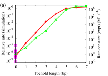
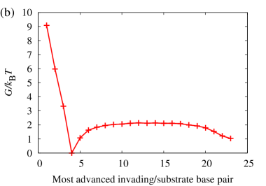
Figure 3: (a) Experimentally measured rate constants as a function of length for an average-strength toehold Zhang_disp_2009 (green ‘x’ symbols), compared to the relative displacement rates found for oxDNA (red ‘+’ symbols, reported relative to the 5 base-pair case) Srinivas2013 . Purple squares show the new estimates of zero-toehold displacement rate for oxDNA presented in this work (detailed in the Supplementary Material), showing substantial measurement uncertainty. Although not quantified here, this uncertainty is much smaller for longer toeholds, when the process is easier to sample Srinivas2013 . The minor variation between rates for long toeholds demonstrates the small error in this limit. (b) Free energy ($G$) profile of displacement in oxDNA as a function of the most advanced invader/substrate base pair for a four-base toehold. Base pair ‘1’ is at the far end of the toehold from the displacement domain, and base pair 4 is immediately adjacent to the displacement domain Srinivas2013 . Typical errors on these measurements are smaller than the ‘+’ symbols, as estimated through comparison of independent simulations Srinivas2013 .

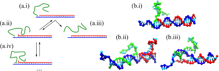
Figure 4: Representations of displacement at two levels of detail. In both cases the substrate is blue, the invader green and the incumbent red. (a) Illustration of a simple step-by-step model of displacement for a one-base toehold. Starting from the toehold-bound state (a.i), either a base pair between incumbent and substrate can break (a.ii) or the toehold base pair can break, leading to detachment (a.iii). From state (a.ii), either the invader can bind to the newly revealed substrate base (a.iii), or the incumbent can rebind, returning us to the initial state (a.i). This process can be repeated for every base in the displacement domain. (b) Displacement in oxDNA (for a three-base toehold). (b.i) The toehold-bound state. (b.ii) A later stage of displacement. (b.iii) A later stage of displacement in which the invader and incumbent duplexes have unstacked at the displacement junction.

III.1 Basic displacement

TMSD was experimentally characterised by Zhang and Winfree Zhang_disp_2009 . These authors demonstrated that for short toeholds, displacement rate increases exponentially with toehold length, before plateauing in the long toehold limit. The results, a subset of which are reproduced in Fig. 3 (a), show that displacement accelerates by a factor of $\sim 10^{6.5}$ as the toehold is increased from 0 to 15 base pairs (for a displacement domain of 20 base pairs, at 25^∘C and with a high salt concentration of [Mg²⁺]$\approx 10$ mM). The overall shape of the graph is unsurprising. At the low strand concentrations used in Ref. Zhang_disp_2009 , the three-stranded intermediate (including states depicted in Figs. 4 (a.ii), (a.iv) and (b)) is short-lived and the reaction is effectively second order. In this limit, the reaction rate constant can be modelled as

$$k_{\rm eff}=k_{\rm bind}P_{\rm suc},$$ (2)

where $k_{\rm bind}$ is a toehold binding rate constant and $P_{\rm suc}$ is the probability that displacement succeeds (as opposed to the invader detaching) once the toehold is formed. For very short toeholds it is reasonable that $P_{\rm suc}\ll 1$. Increasing the toehold length increases the toehold stability, and hence $P_{\rm suc}$, exponentially. Eventually this increase with toehold length saturates when $P_{\rm suc}\sim 1$. Given that $k_{\rm bind}$ would be expected to be relatively weakly length-dependent, $k_{\rm eff}$ therefore plateaus at this point.

A simple argument, however, would suggest that a single-base toehold should have a success rate greater than 1%, thereby limiting the possibilities for increasing $k_{\rm eff}$ by increasing the toehold length and hence $P_{\rm suc}$. Consider the system illustrated in Fig. 4 (a), with a toehold of one base, and assume that displacement is a random walk in which base pairs at the junction can break and then be replaced by base pairs with the competing strand, as shown in Fig. 4 (a). From the toehold-bound state, two things can happen – either the toehold detaches, or the first base pair in the incumbent/substrate breaks. If the latter, the invader then takes a base pair from the incumbent 50% of the time, otherwise the system returns to the initial state. If toehold detachment (involving the disruption of a single base pair), and breaking of base pairs at the junction have similar rates, the probability that the invader manages to take the first step is then approximately 1/3. From here, 19 more displacement steps are required, whereas the initial state is one backwards step away. From the statistics of random walks, we obtain $P_{\rm suc}\sim\frac{1}{3}\frac{1}{20}\sim 0.02$ for single-base toeholds. Given this estimated value of $P_{\rm suc}$ for a single-base toehold, it is difficult to justify the extent of the experimentally observed slowdown for shorter toeholds.

The displacement process has been simulated with oxDNA, as outlined in Ref. Srinivas2013 . The results shown in Fig. 3 (a) agree well with those obtained by Zhang and Winfree. The key point, however, is not the quality of agreement, but that oxDNA also violates the simple argument outlined above which suggests only a modest slowdown for short toeholds. By studying oxDNA, we can then hope to explain the experimental results. Explanations for this behaviour, violations of two assumptions of our simple argument, are given discussed in detail Ref. Srinivas2013 .

Firstly, junction migration is not an unbiased random walk. As junction migration is initiated, a second single-stranded section is generated at the displacement junction, as can be seen in Fig. 4 (b). This second overhang is thermodynamically unfavourable, due to steric exclusions at the junction, and consequently biases the system against initiating and proceeding with junction migration. It therefore reduces the probability of successful displacement given toehold binding. A free-energy profile indicating a thermodynamic cost for initiating displacement is shown in Fig. 3 (b) (the free energy as a function of an order parameter, $G(Q)$, is a measure of the probability that the system exists in state $Q$, $P(Q)$: $G(Q)=-k_{\rm B}T\ln P(Q)+{\rm const}$).

Secondly, simulations show that junction migration is far more complex than the breaking of a single base pair in the toehold, necessarily involving the disruption of more stacking interactions and a greater structural rearrangement. Junction migration is then intrinsically slow compared to the disruption of toehold base pairs, again reducing the probability of displacement as opposed to detaching from the toehold.

The Winfree group have used the thermodynamic stability of ‘frozen’ displacement intermediates to explore the possibility of the penalty associated with dangling ssDNA at the junction, confirming its existence and estimating a value of $\sim 3k_{\rm B}T$, slightly larger than found for oxDNA Srinivas2013 . Analysis of a simple secondary-structure based model Srinivas2013 suggests that such an impediment provides only a partial explanation of the degree to which longer toeholds can accelerate displacement. As a consequence, the second factor identified by oxDNA as inhibiting displacement (slow junction migration) seems necessary to explain the wide range of rates as a function of toehold length.

III.2 Displacement involving mismatches

Figure 5: Relative rates of displacement as a function of the position of a mismatch created during displacement (as predicted by oxDNA) Machinek2014 . The position is defined with respect to the far end of the displacement domain (which has a length of 16 base pairs in this system) – a mismatch at position ‘16’ is immediately adjacent to the toehold, and a mismatch at position ‘4’ is near the far end of the displacement domain. Values are reported relative to the rate for a perfectly matched invader, and the all points are estimated to have an error less than or equal to a factor of 2, as estimated through independent simulations Machinek2014 .

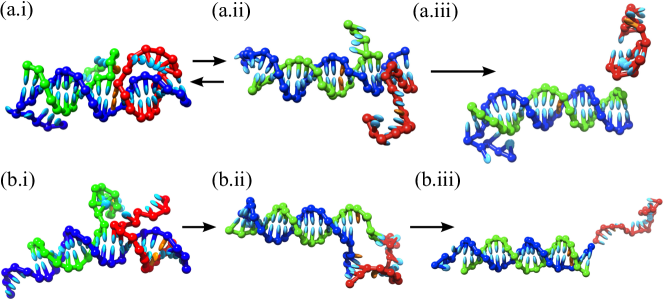
Figure 6: Distinct pathways for displacement involving the creation of a mismatched base pair. The incumbent is shown in red, the invader in green and the substrate in blue. The location of the mismatch is highlighted by the orange-coloured bases. (a) Creating a mismatch in the middle of the displacement domain. The typical pathway involves enclosure of the mismatch (a.ii) prior to detachment of the incumbent and the completion of displacement (a.iii). (b) Creating a mismatch four bases from the end of the displacement domain typically involves detachment of the incumbent (b.ii) prior to enclosure of the mismatch (b.iii).

The plateau in displacement rate as toehold length increases limits the maximal selectivity for intended processes over leak reactions. Modifying displacement to reduce its success probability would enlarge the regime in which rate grows with toehold stability, and hence the dynamic range and maximal selectivity. Authors have included physical separation of the toehold from the displacement domain Genot2011 or forced the invading strand to create unfavourable ‘mismatched’ base pairs Zhangmm2012 ; Jiang2014 to achieve this. The principle is generally to slow displacement by decreasing the overall free-energy gain $|\Delta G^{\rm disp}|$ of the reaction.

OxDNA has been used to simulate displacement in which a C-G base pair is replaced by a C-C mismatch as displacement proceeds Machinek2014 . Mismatches were considered at the start, in the middle, and four base pairs from the end of a 16-base displacement domain, for a toehold of 5 bases. In each case, the mismatch destabilises the final invader/substrate duplex by approximately $\Delta\Delta G^{\rm disp}_{\rm mm}=5.9k_{\rm B}T$. We might then naïvely expect a rate reduction by a factor

$$\frac{k_{\rm eff}^{\rm mm}}{k_{\rm eff}^{\rm perfect}}\approx\exp(-\Delta\Delta G^{\rm disp}_{mm}/k_{\rm B}T)\approx\frac{1}{350}$$ (3)

The results, taken from Ref. Machinek2014 and shown in Fig. 5, are initially surprising. The early mismatch does indeed cause a slowdown by $\sim 350$, and the middle mismatch by a factor $\sim 100$. The late mismatch, however, has almost no influence. This result must mean that $P_{\rm suc}$ is high despite the late mismatch. The fact that the mismatch is far from the toehold certainly helps – after encountering the mismatch, the junction must migrate 12 steps backwards before the invader is bound only to the toehold, raising the probability that displacement will occur anyway despite the impediment. However, mismatches are so destabilising ($5.9k_{\rm B}T$ in this case) that it is still difficult to see how enclosing it and subsequently completing junction migration would not be slow compared to returning to the toehold-only state. The resolution of this paradox is the existence of an alternative pathway, in which the incumbent strand spontaneously detaches from the substrate at a stage when the invader has not yet enclosed the mismatch. This pathway should be contrasted with the standard picture of base-by-base displacement Srinivas2013 . The invader/substrate base pairs beyond the mismatch are then formed at a later stage, when there is no competition from the incumbent, and the full penalty of $\Delta\Delta G^{\rm disp}_{\rm mm}$ is not manifest in the displacement reaction rate. This alternative pathway is illustrated schematically, and contrasted with a displacement pathway which involves enclosing the mismatch, in Fig. 6.

Spontaneous detachment involves breaking a number of base pairs. When the mismatch is late in the displacement domain, it is feasible for the incumbent to detach spontaneously when the invader reaches the mismatch location. This process is somewhat analogous to the detachment of a short toehold, as discussed in Section III.1. As highlighted in Section III.1, toehold detachment is relatively fast compared to completing displacement; this explains why spontaneous detachment involving the disruption of several base pairs can be a kinetically favoured pathway, even when the most stable final state involves enclosure of the mismatch by the invader/substrate duplex.

As the mismatch is moved towards the start of the displacement domain, the number of base pairs that must break spontaneously grows and the rate of detaching in this way is exponentially suppressed. Eventually, spontaneous detachment is so slow that it is no longer faster than simply continuing displacement in the conventional base-by-base manner, and enclosing the mismatch. For oxDNA, both the middle and early mismatches are in this regime and hence they feel the effect of $\Delta\Delta G^{\rm disp}_{\rm mm}$. The difference between middle and early mismatches arises not from differences in the rate at which displacement occurs given toehold binding, but actually due to slower toehold detachment for the middle mismatch Machinek2014 .

In general, oxDNA predicts that mismatches formed at the start of a displacement domain will heavily suppress displacement rates. Rates should initially rise slightly as the mismatch is moved towards the far end of the domain (away from the toehold). At some point, the spontaneous melting pathway will become relevant and the overall rate will rise rapidly, eventually plateauing at the perfectly-matched value. Recent experiments have demonstrated exactly this behaviour Machinek2014 , showing that oxDNA is a powerful tool for probing DNA reaction dynamics.

These results emphasise that mismatches should be placed at the start of the displacement domain to slow displacement and thus suppress the rate of leak reactions. Recent work has considered using displacement to resolve single-nucleotide polymorphisms in genes Li2002 ; Subramanian2011 ; Zhang_disp_2012 ; Chen_disp_2013 ; oxDNA suggests that the simplest kinetic methods might struggle to detect mutations at the end of a displacement domain Li2002 ; Subramanian2011 , although modified approaches might fair better Zhang_disp_2012 ; Chen_disp_2013 . More generally, the results illustrate a mechanism for modulating reaction kinetics by orders of magnitude whilst maintaining approximately the same overall reaction thermodynamics. A corollary is that reverse reactions will be far faster for the late mismatch, which may also be important when designing nanotechnological systems.

III.3 Displacement during the cycle of a burnt-bridges motor

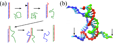
Figure 7: The burnt-bridges motor introduced in Ref. Bath2005 . (a) A schematic of of motor operation. The cargo (red) is initially bound to the first stator (blue). A nicking enzyme cuts this stator, revealing a toehold (six bases in this case) for an alternative stator (green) which can displace the original, resulting in a step of the cargo strand. (b) An intermediate stage of stepping as represented by oxDNA. The two stators are anchored at points indicated by the vertical arrows. From this figure it is clear that the final stages of displacement involve subjecting the motor to considerable tension as it stretches between the two anchoring points.

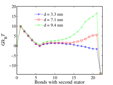
Figure 8: Free-energy ($G$) profiles as a function of the number of bonds with the second stator during the displacement stage of the cycle of a burnt-bridges motor. Profiles are shown for three different separations between the anchoring points of the stators. Reprinted with permission from P. Šulc et al., Simulating a burnt-bridges DNA motor with a coarse-grained DNA model, Natural Computing 1-13. Copyright (2013) Springer Science and Business Media Sulc_walker_2012 .

OxDNA has been used Sulc_walker_2012 to model a burnt-bridges DNA motor designed by Turberfield and coworkers Bath2005 ; Wickham2011 ; Wickham2012 . The motor is illustrated in Fig. 7 (a). I will focus on the mechanism by which the motor strand (or ‘cargo’) steps from one stator (a single-stranded binding site anchored to the track) to the next via displacement - a simulation snapshot of this process is shown in Fig. 7 (b). The free-energy profiles of displacement, for various distances $d_{s}$ between the stators, are shown in Fig. 8. As $d_{s}$ is increased, toehold formation becomes slightly less favourable, due to a greater loss of entropy associated with toehold binding when the stators are further apart. Far more significant, however, is the rise in free energy at later stages that can be seen for large $d_{s}$. As displacement progresses, fewer bases are available to stretch across the gap between the points at which the stators are anchored, as shown in Fig. 7 (b). Displacement must then work against the tension of these stretched bases, meaning that the free energy rises as displacement progresses.

Some caution must be exercised when using free-energy profiles to infer kinetics. If the low-dimensional order parameter used is not a perfect reaction coordinate, signatures of kinetic effects may be hidden. Indeed, the relative difficulty of junction migration highlighted in Section III.1 is not easily identified in free-energy profiles at the level of base pairs. Nonetheless, large stator separation will clearly frustrate motor stepping, primarily due to lower rates of displacement once the toehold is formed, rather than slow toehold formation. Moderately large stator separations could then be used like early mismatches to reduce displacement success probabilities, thereby increasing the toehold length required to saturate $P_{\rm suc}$ at unity and suppressing leak reactions relative to the rate in this long-toehold limit. This approach would be particularly useful at junctions where decisions must be made Wickham2012 . If $d_{s}$ primarily influenced binding rates, rather than success probabilities, larger $d_{s}$ would not help to discriminate between toeholds but would slow all reactions equally.

It is worth noting that slowing displacement by increasing $d_{s}$ alters reaction kinetics without changing the overall $\Delta G$ of reaction. This is similar to changing the location of a mismatch formed between invader and substrate, but unlike increasing the number of mismatches. This is because the initial and final states, in which the cargo is bound to one stator only, are not $d_{s}$-dependent. Large values of $d_{s}$ can in principle be used at an arbitrarily large number of stages for the same cargo molecule without destabilising the final product. This advantage of modulating kinetics with $d_{s}$ must be weighed against the fact that the motif is limited to sequential reactions on a surface.

IV Recovery of a two-footed walker: an example of enhanced displacement

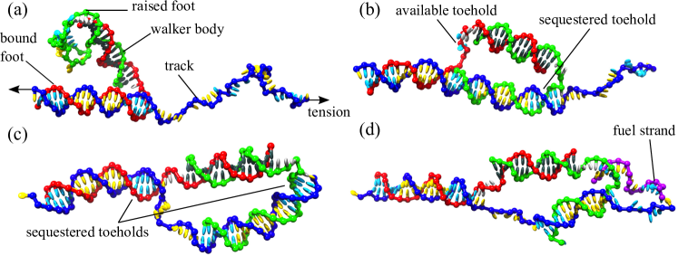
Figure 9: States relevant to the operation of a two-footed DNA walker. The backbone of the track is coloured blue, the two feet red and green and the fuel purple. Bases are coloured according to their ‘domain’ – sky blue bases are toehold sequences, and yellow bases constitute the longer binding domains between track and foot. Dark green bases form the duplex that holds the two feet together. The system has an inherent asymmetry which allows the definition of forward and backward directions Ouldridge_walker_2013 ; in this figure, the forward direction is to the right. (a) Walker with one foot bound to the back site of a three-site track. (b) Walker bound to two adjacent sites on a three-site track, revealing a toehold for the fuel to raise the back foot. (c) Overstepped walker with sequestered toeholds. (d) Fuel displacing the track from the foot, prior to recovery of the walker from the overstepped state. In all figures, the track is subject to a tension of 14.6 pN in the horizontal direction.

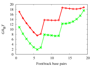
Figure 10: Free-energy profile $G$ for the raising of the front foot of an overstepped walker, given at least one base pair between an invading fuel strand and the foot. Data is shown for systems both with (green ‘x’ symbols) and without (red ‘+’ symbols) a tension of 14.6 pN applied the track. Free energies are measured relative to a reference state in which the fuel is yet to bind. Increasing displacement corresponds to reduced numbers of base pairs between foot and track - i.e., moving from right to left on the graph. Large jumps at 7-8 and 12-13 are due to the repairing of mismatches by the invader; these mismatches are present by design to prevent enzymatic cleavage of the track. Statistical errors are similar in magnitude to the size of symbols; a more detailed discussion is given in the Supplementary Information.

The Turberfield group has also introduced a two-footed DNA walker that is designed to achieve directional motion without modifying its track, a continuous single strand consisting of multiple binding sites Bath2009 . The walker is intended to step in a foot-over-foot fashion; its full design is given in Ref. Bath2009 . It is intended to exist either with a single foot bound to the track and the other raised, or with both feet bound to overlapping adjacent sites, as illustrated in Fig. 9 (a) and (b). The feet must overlap, as competition means that one or other of the feet will then have a raised toehold domain. A single-stranded fuel can bind to this raised domain, initiating displacement of the track and raising the foot. The fuel is designed to selectively raise the ‘back’ foot due to asymmetry within the system.

An earlier oxDNA study Ouldridge_walker_2013 revealed that the walker had a tendency to ‘overstep’, or bind to two non-adjacent sites (Fig. 9 (c)). This is disastrous for the walker, leaving both feet bound to the track without a free toehold to initiate foot-lifting. This tendency was observed even with tracks under moderate tension ($\sim 15$ pN). Although tension could not prevent overstepping, increased disruption (fraying) of the front foot/track duplex hinted that recovery might be easier in the presence of tension, due to destabilisation of the overstepped state.

I now present evidence that tension does facilitate recovery from the overstepped state. I simulate toehold-free (blunt-ended) displacement of the track from the overstepped foot by a fuel molecule, as illustrated in Fig. 9 (d), both with and without a tension of 14.6 pN applied to the track. Langevin Dynamics simulations enhanced by FFS are used to estimate relative rates, and free-energy profiles of displacement are estimated using VMMC aided by US. Full methodological details are provided in the Supplementary Information. Kinetic simulations indicate that displacement is $\sim 5\times 10^{3}$ faster with tension than without, and the free-energy profiles (Fig. 10) show that a difference of about $\Delta\Delta G_{\rm tension}\approx 6.4k_{\rm B}T$ develops between the two systems as displacement progresses.

When bound to two non-adjacent sites as in Fig. 9 (c), the walker tends to constrain the track and reduce its possible extension. Importantly, as individual base pairs between the forward edge of the front foot and the track are disrupted, the track is able to extend incrementally further (see Fig. 9 (d)). As a consequence, these base pairs break more easily than without tension – they have a higher tendency to be frayed prior to fuel binding, providing an effective toehold for displacement. Further, because base pairs with the fuel are more stable than with the track, displacement of the track is biased towards success (as evidenced by the slope at the start of displacement in Fig. 10 for the system under tension). Detailed inspection of the FFS results indicates that faster displacement is due to both easier binding and a higher subsequent probability of displacement success. If the thermodynamic results were used to estimate relative rates via $\exp(-\Delta\Delta G_{\rm tension}/k_{\rm B}T)$, a value of approximately 600 would be obtained. The statistical errors associated with the kinetic estimates in particular are substantial, so it is possible that the difference is due to random error. However, it is also possible that the free-energy profile fails to highlight subtle kinetic effects, such as those that were observed in conventional displacement. Regardless, the two results clearly predict a substantial increase in walker recovery rate of $\sim 10^{3}$ or more under the application of moderate tension.

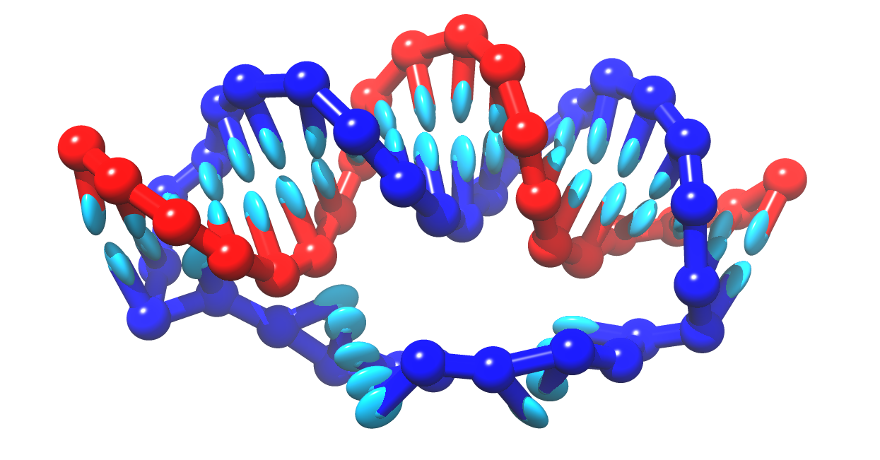
Figure 11: Generating tension that will favour displacement in a “self contained” manner by using a short circular strand as the incumbent.

The fact that tension can aid walker recovery highlights the possibility of building contingency into nanodevice operation, thereby allowing for fail-safe behaviour. It also demonstrates the possibility of enhancing displacement through tension, an alternative way to modulate kinetics. In this case, tension is externally applied to the track; one possibility is to stretch the track between two points of an origami structure. One could generate tension in a more self-contained way by using circular substrates, as shown in Fig. 11; indeed, similar constructs have been studied experimentally Hao2011 ; Wang2013 . Here, a sufficiently long duplex section will apply an extensional stress to a sufficiently short single-stranded section, and will experience a compression in response, leading to the bending shown in Fig. 11. Displacement rates in such a system could be modulated by secondary structure within, or binding to, the single-stranded loop of the substrate - this modulation would be freed from any constraints of the invader sequence.

V Discussion

DNA nanotechnology has enormous potential, but providing a solid theoretical underpinning is vital if it is to truly flourish. This understanding can be achieved through a combination of careful experimentation and modelling. Certain groups are now taking up the challenge of meticulously understanding the processes involved by carefully measuring important reactions in a variety of contexts Zhang_disp_2009 ; Sobczak2012 ; Myhrvold2013 ; Ke2012b ; Martin2012 ; Tomov2013 ; Johnson-Buck2013 ; Tsukanov2013 . In this article I have discussed a coarse-grained model of DNA, oxDNA, that can complement these efforts. OxDNA is an attempt to incorporate the thermodynamics of DNA as parameterised by SantaLucia’s nearest-neighbour model into a structural and mechanical framework consistent with current knowledge. It can then be used to study the behaviour of ‘ideal’ DNA, exploring the possibilities of certain motifs, testing whether new experimental observations are consistent with current understanding, and revealing which properties of DNA have an influence on certain phenomena.

I have reviewed a number of applications of oxDNA, demonstrating that it provides quantitative understanding of aspects of displacement processes and can offer qualitative insight into reaction mechanisms and novel motifs. In each case, a physically reasonable underlying cause for the observation in question was identified, such as stress that is generated or relieved during displacement. These effects should therefore be manifest in real DNA, rather than simply being artefacts the model or simulation technique. Intriguing questions remain open, as there are many possible motifs available for study. For example, displacement reactions have recently been reported in the context of unconventional left-handed super-helices formed by conventional B-DNA domains in a complex pseudoknotted structure Li2014 – such a system would an ideal candidate for study with oxDNA. Other possibilities include studying the influence of single-stranded hairpins, which are frequently present both by accident and design, on hybridisation and displacement kinetics, and considering general properties of displacement cascades on surfaces Teichmann2014 .

oxDNA’s strengths are its efficiency and good overall representation of the structural, mechanical and thermodynamic changes associated with short duplex formation. To achieve efficiency, however, the description of nucleotides is extremely simple and electrostatics in particular is treated in a basic fashion. Some properties, such as the opening of internal denaturation bubbles and the structures of systems that are more complex than simple duplexes, are yet to be fully tested against experimental data. Characterising and improving these limitations will be the subject of further work.

oxDNA is parameterised to experimental data on the basic properties of DNA, but experimental results are not unequivocal. In particular, the typical state, stacking propensity and conformation of single strands are poorly understood (as discussed in Refs. Ouldridge2011 ; Ouldridge_thesis ), with some authors even finding evidence for structure formation when none would be expected from Watson-Crick base pairing Sikora2013 . Single strands have an enormous role in nanotechnological systems, not least as the initial state of the hybridisation process, which itself is not unambiguously understood. Particularly pertinent open questions relate to the temperature-dependence of hybridisation, as discussed in Ref. Ouldridge_binding_2013 , and its behaviour near a surface Johnson-Buck2013 . Mechanical properties of duplexes, and whether DNA can be described as a wormlike-chain at short length scales, are still the subject of debate Wiggins2006 ; Vafabakhsh2012 ; Vologodskii2013 ; Mazur2014 . Resolving these fundamental issues would be extremely useful in nanotechnology and beyond. It is likely that, as further characterisation is performed, some of the assumptions inherent in the current understanding of DNA (and hence oxDNA) will have to be revisited.

In this article I have focussed on the application of oxDNA to small, active systems. oxDNA has also been used to study DNA in a range of other contexts, including large duplexes under applied stress Doye2013 , and self-assembly driven phase transitions Rovigatti2014 ; Rovigatti2014b . A modified version parameterised to describe RNA has recently been developed Sulc2014 . Although some progress has been made with improving the experimental protocols for constructing large structures Sobczak2012 ; Myhrvold2013 ; Ke2012b ; Martin2012 , the assembly pathways and systematic ways to optimise them remain elusive. Modelling the assembly of larger structures with oxDNA is a current goal, but remains extremely challenging due to the large number of rare-event binding processes that must be observed. Further development and refinement of enhanced dynamic sampling techniques, such as FFS, would assist in this process. It may be that oxDNA can best be used to study smaller sub-structures, and that this information can then be incorporated into models at the level of secondary structure Dirks2007 ; Schaeffer_thesis or whole binding domains Phillips2009 ; Arbona2013 ; Reinhardt2014 .

Appendix A Simulation methods

Thermodynamic properties of model DNA are obtained by averaging over the Boltzmann distribution

$$\rho({\bf r}^{N},{\bf p}^{N},{\bf q}^{N},{\bf L}^{N})\hskip 5.69054pt\propto\hskip 5.69054pt\exp({-\beta\mathcal{H}({\bf r}^{N},{\bf p}^{N},{\bf q}^{N},{\bf L}^{N})}),$$ (S4)

where $\mathcal{H}$ is the system Hamiltonian, ${\bf r}$ and ${\bf q}$ are positional and orientational degrees of freedom and ${\bf p}$ and ${\bf L}$ are linear and angular momenta. The momenta can be separately integrated analytically, and thus the relative probability of a configuration is given simply by $\exp(-\beta V({\bf r}^{N},{\bf q}^{N}))$. For oxDNA, thermodynamic averages are typically calculated using the Virtual Move Monte Carlo (VMMC) algorithm.Whitelam2007 ; Whitelam2009 Dynamical studies reported in this work use a Langevin Dynamics (LD) algorithm for rigid bodies,Davidchack2009 which samples from the Boltzmann distribution and generates diffusive particle motion.

A.1 VMMC

VMMCWhitelam2007 ; Whitelam2009 is a cluster-based Monte Carlo technique that is particularly effective for dilute systems with strong, directional interactions such as oxDNA. Results reported in this work use the variant introduced in the appendix of Ref. Whitelam2009, . The algorithm involves attempting moves of particle clusters that are generated in a way that reflects potential energy gradients in the system, and accepting these attempted moves with a probability that ensures the system samples from the canonical ensemble. As clusters of strongly interacting particles move together, VMMC equilibrates oxDNA systems much more efficiently than traditional Monte Carlo algorithms.

‘Seed’ moves of a single particles are used to explore the energy gradients in a system and generate clusters. For all the VMMC simulations reported in this work, the seed moves were;

• rotation of a nucleotide about its backbone site, with the axis chosen from a uniform random distribution and the angle from a normal distribution with mean of zero and a standard deviation of 0.12 radians.

• translation of a nucleotide with the direction chosen from a uniform random distribution and the distance from a normal distribution with mean of zero and a standard deviation of 1.02 Å.

A.1.1 Umbrella Sampling

Many processes (such as the binding of two strands) are slow to equilibrate, despite the simplicity of oxDNA and the efficiency of VMMC as a simulation technique. Slow equilibration often arises when the system has multiple competing local minima of free energy, separated by large free-energy barriers. An artificial biasing weight $W({\bf r}^{N},{\bf q}^{N})$ can be used to enhance equilibration by flattening these barriers.Torrie1977 This procedure, known as Umbrella Sampling (US), involves choosing $W({\bf r}^{N},{\bf q}^{N})$ to favour the states of high free energy that must be crossed to pass between the free energy minima. The expectation of any variable $A$ can be extracted from these biased simulations via

$$\langle A\rangle=\frac{\langle A({\bf r}^{N},{\bf q}^{N})/W({\bf r}^{N},{\bf q}^{N})\rangle_{W}}{\langle 1/W({\bf r}^{N},{\bf q}^{N})\rangle_{W}}.$$ (S5)

Here, $\langle\rangle_{W}$ indicates sampling from the biased ensemble in which states are visited with a probability proportional to $W({\bf r}^{N},{\bf q}^{N})\exp(-\beta V({\bf r}^{N},{\bf q}^{N}))$. It is often helpful to define a (low-dimensional) order parameter $\psi({\bf r}^{N},{\bf q}^{N})$ that describes the process in question, and to then define the bias $W(\psi)$ using this order parameter rather than through the individual coordinates.

A.1.2 The Weighted Histogram Analysis Method

Even with Umbrella Sampling it can be challenging to sample all relevant states of a system within a single simulation. It is sometimes advantageous to split the simulations into overlapping ‘windows’ of state space that can be separately equilibrated more easily. The data from the individual windows can be combined to give the statistical properties of the whole system by relating the windows using the overlapping regions. One systematic approach to achieve this is known as the ‘Weighted Histogram Analysis Method’ (WHAM).Kumar1992 To use the WHAM algorithm, one must supply

• $W^{i}(\psi)$, the biasing potential used in window $i$.

• $\rho^{i}(\psi)$, the normalised distribution measured during simulation window $i$.

• $n^{i}$, the total number of VMMC steps taken over all simulations in window $i$.

The WHAM algorithm takes these inputs and iteratively estimates the overall distribution $\rho(\psi)$ and the dimensionless free-energy of window $i$ ($F_{i}$), via the equations

$$\begin{array}[]{c}\rho^{\prime}(\psi)=\frac{\sum_{i}\rho^{i}(\psi)n^{i}}{\sum_{i}n^{i}\exp(F_{i})W^{i}(\psi)},\\ \\ \rho(\psi)=\frac{\rho^{\prime}(\psi)}{\sum_{\psi}\rho^{\prime}(\psi)},\\ \\ \exp(-F^{i})=\sum_{\psi}W^{i}(\psi)\rho(\psi).\\ \end{array}$$ (S6)

From an initial (trivial) choice of $F_{i}$, the measured data can be used to iterate these equations until convergence, resulting in an overall estimate of the unbiased occupancy of individual states, $\rho(\psi)$.

A.2 Langevin Dynamics

LD allows Newton’s equations of motion for the particles that are explicit in the model to be augmented with random and dissipative forces due to an implicit solvent. These forces are chosen so that particles move diffusively and the system samples from the Boltzmann distribution. The kinetic results reported in this work were obtained using the quaternion-based algorithm for rigid bodies of Davidchack et al.Davidchack2009 Other work on oxDNA has been performed with an Andersen-like thermostat.Russo2009

To use the LD algorithm, a nucleotide mass (which is taken as $m=315.75$ Da for all nucleotides) and a moment of inertia tensor (we treat the nucleotides as spherical with a moment of inertia $31.586$ Da nm²) are required.Ouldridge_thesis The drag forces experienced by a particle must also be related to its generalised momenta via a friction tensor. We ignore the complexity of hydrodynamic coupling between particles. For simplicity, we treat each nucleotide’s interaction with the solvent as spherically symmetric which means that only linear and rotational damping coefficients $\gamma$ and $\Gamma$ remain as independent quantities. The investigations reported in this paper use values of $\gamma=0.59$ ps^-1 and $\Gamma=1.76$ ps^-1. These values result in diffusion coefficients of $D_{\rm sim}=1.91\times 10^{-9}$ m²s^-1 for a 14 base-pair duplex, higher than experimental measurements of $D_{\rm exp}=1.19\times 10^{-10}$ m²s^-1.Lapham1997 Accelerating diffusion in this manner allows simulations to explore more complex processes for a given CPU time. Our group has previously shownOuldridge_binding_2013 that increased friction coefficients have almost no qualitative consequences for hybridization pathways in oxDNA, only an overall reduction in the reaction rate. LD Simulations in this work use an integration time step of 8.55 fs, which has been previously shown to reproduce the energies and kinetics obtained with shorter time steps for oxDNA.Ouldridge_thesis

In the studies reported in this work, I compare the measured rates of similar processes; typically, displacement rates as certain system parameters are changed. For such comparisons, the effects of the choice of dynamical method should be approximately the same in each case, meaning that relative rates should be reasonably insensitive to the details of the dynamical algorithm. Furthermore, the numerical results are made meaningful by identifying the physically reasonable factors that lead to them, rather than just reporting the results in isolation.

A.2.1 Forward flux sampling

‘Brute force’ LD simulations are often not efficient enough to sample rare transitions accurately. Forward Flux Sampling (FFS) can be used to enhance the calculation of the flux between two local free-energy minima, and improve sampling from the trajectories that link the two regions (reactive trajectories).Allen2005 ; Allen2009 Here I outline the general method; our specific implementation is detailed in Section C.

Firstly I define the term ‘flux’. Let $A$ and $B$ be two non-overlapping regions of phase space. The flux from $A$ to $B$ is defined in the following way.

For an infinitely long simulation, the flux of trajectories from $A$ to $B$ is $\Phi_{AB}=N_{AB}/{(\tau f_{A})}$, where $N_{AB}$ is the number of times the simulation leaves $A$ and then reaches $B$ without first returning to $A$, ${\tau}$ is the total simulation time and $f_{A}$ is the fraction of simulation time during which the system visited state $A$ more recently than state $B$.

The concept of flux generalises a transition rate for processes that are not absolutely instantaneous.

To use FFS, a one-dimensional discrete order parameter $Q$ is required so that non-intersecting interfaces $\lambda^{n}_{n-1}$ exist between consecutive values of $Q$. The lowest value of $Q$, $Q=-2$, defines state $A$, and the highest value $Q=Q_{\rm max}$ state $B$. Initially, a simulation is performed in the vicinity of $Q=-2$, and the flux of trajectories from $Q=-2$ to $Q=0$ is measured (in effect, one counts the trajectories that cross the surface $\lambda^{0}_{-1}$ for the first time since leaving $Q=-2$). I choose to define the lowest value of $Q$ as $Q=-2$ because the algorithm is distinct for values of $Q>0$.

The total flux of trajectories from $A$ to $B$ then follows as the flux across $\lambda^{0}_{-1}$ from $Q=-2$, multiplied by the conditional probability that these trajectories subsequently cross the interface $\lambda_{Q_{\rm max}-1}^{Q_{\rm max}}$ to reach $Q=Q_{\rm max}$ instead of returning to $Q=-2$, $P(\lambda_{Q_{\rm max}-1}^{Q_{\rm max}}|\lambda_{-1}^{0})$. This probability can itself be expressed as a product of the success probabilities associated with reaching the next interface (rather than returning to $Q=-2$) for each intermediate case, $P(\lambda_{Q-1}^{Q}|\lambda_{Q-2}^{Q-1})$:

$$P(\lambda_{Q_{\rm max}-1}^{Q_{\rm max}}|\lambda_{-1}^{0})=\prod_{Q=1}^{Q_{\rm max}}P(\lambda_{Q-1}^{Q}|\lambda_{Q-2}^{Q-1}).$$ (S7)

In this work, the ‘direct’ FFS approach was used to calculate the product in Equation S7. In this method, a flux simulation is run to calculate the flux from $Q=-2$ to $Q=0$, and generate states at the $\lambda^{0}_{-1}$ interface. These states are used as starting points for estimating $P(\lambda_{0}^{1}|\lambda_{-1}^{0})$. The process is then iterated for subsequent interfaces, using the successes from the previous stage as initial configurations for the next. The branched trajectories obtained sample from the distribution of reactive trajectories. The procedure is illustrated schematically in Fig. S12.

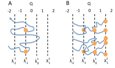
Figure S12: Schematic illustrations of FFS. An order parameter $Q$ is defined with interfaces $\lambda$ separating distinct value of $Q$. We are interested in measuring the flux from $Q=-2$ to $Q=2$ in this example. A) The initial measurement of flux across the interface $\lambda^{0}_{-1}$. Orange dots indicate the crossings that contribute to the flux, and also the states used to launch subsequent stages of simulation. B) Direct FFS involves randomly launching many trajectories from the interface $\lambda^{0}_{-1}$, and measuring the probability of reaching $\lambda^{1}_{0}$ before returning to $\lambda^{-1}_{-2}$. This procedure is then repeated for successive interfaces, resulting in branched trajectories. Reprinted by Permission from T. E. Ouldridge et al., DNA hybridization kinetics: zippering, internal displacement and sequence dependence, Nucleic Acids Research 41:8886-8895. Copyright (2013) Oxford University Press.Ouldridge_binding_2013

Strand	Sequence ($5^{\prime}$–$3^{\prime}$)
Substrate	GAC ATG GAG ACG TAG
	GGT ATT GAA TGA GGG
Incumbent	TCC CTC ATT CAA TAC CCT ACG
Invader	CC CTC ATT CAA TAC CCT ACG

Table S1: Sequences used to simulate zero-toehold displacement. Italic regions indicate the displacement domain.

Strand	Sequence (5′ – 3′)
Track (3 sites)	CAGCATCCT̂TCAGCT̂TCAGCATCCT̂TCAGCT̂TCAGCATCCT̂TCAGCT̂TCAGCATCC
Walker 1	GTATTATCGTTAGTCTttttGATGCTGAĜGCTGAĜGGATGCT
Walker 2	AGACTAACGATAATACttttGATGCTGAĜGCTGAĜGGATGCT
Fuel	CCTCAGCCTCAGCATC

Table S2: Sequences used for simulating the DNA walker. Complementary regions are highlighted in the same colour (corresponding to the colours used for the base sites in Fig. 9 of the main text). The toehold domains are highlighted in blue, and the longer binding domains in yellow. The duplex that holds the walker together is shown in green. Circumflexes indicate mismatched bases between the foot and track (which prevent the track from being cleaved by nicking enzymes in experiment, and also favour foot-lifting by the fuel). Although the fuel can in principle bind to either toehold of both walker strands, only the 5^′ end will naturally lead to displacement.

A.2.2 Error estimation

In the initial work on FFS, the authors suggested calculating statistical error by treating each stage of the simulation as independent attempt to estimate a probability $P(\lambda_{i}^{i+1}|\lambda_{i-1}^{i})$ through a number of independent trials. Such an approach gives the variance in the measured value of $P(\lambda_{i}^{i+1}|\lambda_{i-1}^{i})$ as

$$\sigma_{i}^{2}=P(\lambda_{i}^{i+1}|\lambda_{i-1}^{i})(1-P(\lambda_{i}^{i+1}|\lambda_{i-1}^{i}))/N_{i},$$ (S8)

where $N_{i}$ is the number of trials launched from interface $i$. The overall variance in the flux measurement would then follow by summing the individual variances from each stage.

Order parameter	Distance	Nearly-formed	Number of base pairs	Number of base pairs	Distance
$Q$	$d$/nm	base pairs $n$	$A$ with $E<-2.98$ kcal mol-1	$B$ with $E<-2.98$ kcal mol-1	$d_{2}$/nm
-2	$d>5.11$	$\sim$	$\sim$	$\sim$	$\sim$
-1	$5.11>d>3.41$	$\sim$	$\sim$	$\sim$	$\sim$
0	$3.41>d>2.56$	$\sim$	$\sim$	$\sim$	$\sim$
1	$2.56>d>1.70$	$\sim$	$\sim$	$\sim$	$\sim$
2	$1.70>d>0.852$	$\sim$	$\sim$	$\sim$	$\sim$
3	$0.852>d$	0	0	$\sim$	$\sim$
4	$\sim$	1	0	$\sim$	$\sim$
5	$\sim$	$\sim$	$A=1$	$\sim$	$\sim$
6	$\sim$	$\sim$	$\sim$	$1<B<4$	$\sim$
7	$\sim$	$\sim$	$\sim$	$4<B<20$ or ($B=20$ & $d_{2}<2.56$)
8	$\sim$	$\sim$	$\sim$	$B=20$	$d_{2}\geq 2.56$

Table S3: Order parameter definition for FFS simulations of blunt-ended displacement. $d$ and $d_{2}$ are minimum distances within certain sets of pairs of bases, measured as the separation of hydrogen-bonding sites of a pair. “Nearly-formed” base pairs are defined in the text. The pairs of bases considered for $d$, $n$ and $A$ are only the 3 base pairs at either end of the intended invader/substrate duplex. $B$ includes all intended base pairs in the invader/substrate duplex. $d_{2}$ includes all base pairs in the original incumbent/substrate duplex. “$\sim$” indicates that no additional restriction is placed on this collective degree of freedom that is not covered by other explicitly stated requirements.

Number of replicas	10
Number of simulations per	10
replica for flux across $\lambda^{0}_{-1}$
Initialisation time	85.5
per simulation /ns
Total crossings of $\lambda^{0}_{-1}$	10000
(total time taken/$\mu$s)	181
Average flux across $\lambda^{0}_{-1}$/$\mu$s-1	55.2
Target interface	Total states loaded/successes
$\lambda^{1}_{0}$	100000/41957
$\lambda^{2}_{1}$	100000/42826
$\lambda^{3}_{2}$	100000/21010
$\lambda^{4}_{3}$	100000/ 14469
$\lambda^{5}_{4}$	800000/41467
$\lambda^{6}_{5}$	400000/12297
$\lambda^{7}_{6}$	200000/2797
$\lambda^{8}_{7}$	5000/267
Overall flux to	0.0149
full displacement/s-1	0.026
(individual replica	0.00482
estimates)	0.0356
	0.000975
	0.00362
	0.0220
	0.0200
	0.00475
	0.139

Table S4: Simulation details and data obtained from FFS simulations of blunt-ended displacement.

Our group followed this approach in Refs. Ouldridge_walker_2013, and Srinivas2013, . However, this method underestimates the true variability of the final result, as it assumes that the initial configurations at each interface are a truly representative ensemble. In some cases, particularly when bottlenecks appear in the process, this assumption can be poorly justified. For example, analysis of the simulation results for the zero-toehold displacement presented in Ref. Srinivas2013, showed that only a few of the initial configurations obtained at the $\lambda^{0}_{-1}$ interface subsequently spawned trajectories that led to complete displacement, raising the possibility that the true uncertainty in the result is much higher than suggested.

An alternative approach is to estimate statistical errors by running a number of completely separate FFS protocols and comparing the independent estimates of the overall flux. I have used this procedure for the simulations of walker recovery presented in this work. To check the reliability of our earlier result on TMSD, I also present data for zero-toehold displacement obtained using this approach in the main text. Overall, although error estimates may have been too small, the physical conclusions drawn from earlier work are robust.

Appendix B Systems

B.1 Zero-toehold displacement

Simulations of zero-toehold displacement used the same setup as Ref. Srinivas2013, . Simulations involved one invader, one substrate and one incumbent in a periodic cubic cell of $1.67\times 10^{-20}$ l (litres), at a temperature of $T=298.15$ K. Table S1 contains strand sequences. As in the original work,Srinivas2013 the sequence-independent version of oxDNA was used, and only base pairs native to the initial incumbent/substrate and final invader/substrate duplexes were assigned non-zero binding strength. This simplification eliminates the metastable misbonded configurations, which can hamper FFS without significantly affecting system behaviour.Srinivas2013 The sequence-independent parameterisation of oxDNA can simplifies results as it shows only the generic behaviour of DNA, rather than sequence-specific effects.

Appendix C Simulation protocols

Order parameter	Distance	Nearly-formed	Number of base pairs	Number of base pairs
$Q$	$d$/nm	base pairs $n$	$A$ with $E<E_{A}$	$B$ with $E<E_{B}$
-2	$d>6.81$	$\sim$	$\sim$	$\sim$
-1	$6.81>d>5.11$	$\sim$	$\sim$	$\sim$
0	$5.11>d>4.26$	$\sim$	$\sim$	$\sim$
1	$4.26>d>3.41$	$\sim$	$\sim$	$\sim$
2	$3.41>d>2.56$	$\sim$	$\sim$	$\sim$
3	$2.56>d>1.70$	$\sim$	$\sim$	$\sim$
4	$1.70>d>0.852$	$\sim$	$\sim$	$\sim$
5	$0.852>d$	0	0	0
6	$\sim$	1	0	0
7	$\sim$	$\sim$	($A\geq 1$  & $B=0$) or ($A=1$  & $B=1$ )
8	$\sim$	$\sim$	($A\geq 2$  & $B=1$) or ($A=2$  & $B=2$ )
9	$\sim$	$\sim$	$A\geq 3$	$4>B\geq 2$
10	$\sim$	$\sim$	$\sim$	$16>B\geq 4$
11	$\sim$	$\sim$	$\sim$	16

Table S5: Order parameter definition for FFS simulations of walker recovery by fuel displacement. $d$ is the minimum distance between bases that are intended to form base pairs in the final invader/substrate duplex, measured as the separation of hydrogen-bonding sites. “Nearly-formed” base pairs are defined in the text. All base-pairing contributions to the order parameter include only those base pairs that are intended to be present in the final invader/substrate duplex. $E_{A}=-1.43$ kcal mol^-1 and $E_{B}=-1.79$ kcal mol^-1. “$\sim$” indicates that no additional restriction is placed on this collective degree of freedom that is not covered by other explicitly stated requirements.

System	With tension	Without tension
Number of replicas	10	10
Number of simulations per	10	10
replica for flux across $\lambda^{0}_{-1}$
Initialisation time	2.565	2.565
per simulation /$\mu$s
Total crossings of $\lambda^{0}_{-1}$	2557	3090
(total time taken/$\mu$s)	94.2	126
Average flux across $\lambda^{0}_{-1}$/$\mu$s-1	27.1	24.5
Target interface	Total states loaded/successes
$\lambda^{1}_{0}$	40000/18156	40000/17850
$\lambda^{2}_{1}$	39803/21181	38975/20341
$\lambda^{3}_{2}$	37600/21154	39947/22017
$\lambda^{4}_{3}$	40000/22095	40000/21060
$\lambda^{5}_{4}$	71200/20636	76000/18448
$\lambda^{6}_{5}$	40000/9708	80000/11296
$\lambda^{7}_{6}$	99000/3353	200000/1744
$\lambda^{8}_{7}$	37939/5869	200000/5878
$\lambda^{9}_{8}$	20000/3981	160000/2629
$\lambda^{10}_{9}$	5000/2137	30000/5105
$\lambda^{11}_{10}$	1880/909	3880/773
Overall flux to	135	0.00438
full displacement/s-1	37.1	0.00340
(individual replica	45.5	0.0332
estimates)	32.3	0.00131
	58.1	0.00384
	7.96	0.00492
	1.49	0.00987
	47.9	0.01345
	18.3	0.00376
	11.3	0.00167

Table S6: Simulation details and data obtained from FFS simulations of walker recovery.

C.1 Overstepped walker recovery

Walker simulations involved the two strands that constitute the walker itself, a track containing three binding sites with one extra base at either end to limit the effects of truncating the track, and a fuel strand in a periodic cubic cell of $7.73\times 10^{-20}$ l. Table S2 displays the sequences. A temperature of 310 K was used, close to experimental conditions.Bath2009 For simulations involving tension, a constant force of 14.6 pN was applied to the backbone sites at either end of the track. Consistent with earlier work on the walker using oxDNA,Ouldridge_walker_2013 the sequence-independent parameterisation of oxDNA was used. To simplify sampling, only expected interstrand bonds (i.e., those intended in the design) were assigned non-zero binding strength, although any intrastrand base-pairing was allowed.

	$\psi_{2}=0$, $\psi_{3}=$				$\psi_{3}=3$, $\psi_{2}=$
$\psi_{1}$	0	1	2	3	1	2	3	4	5	6	7	8	9	10	11	12	13	14	15	16
0	0	0	0	0	0	0	0	0	0	0	0	0	0	0	0	0	0	0	0	0
1	1	20	500	4000	$1.2\times 10^{8}$	$1.2\times 10^{8}$	$1.2\times 10^{8}$	0	0	0	0	0	0	0	0	0	0	0	0	0
2	1	20	500	4000	$1.2\times 10^{8}$	$1.2\times 10^{8}$	$1.2\times 10^{8}$	0	0	0	0	0	0	0	0	0	0	0	0	0
3	1	20	500	4000	$1.2\times 10^{8}$	$1.2\times 10^{8}$	$1.2\times 10^{8}$	0	0	0	0	0	0	0	0	0	0	0	0	0
4	1	20	500	4000	$1.2\times 10^{8}$	$1.2\times 10^{8}$	$1.2\times 10^{8}$	0	0	0	0	0	0	0	0	0	0	0	0	0
5	1	20	500	4000	$1.2\times 10^{8}$	$1.2\times 10^{8}$	$1.2\times 10^{8}$	0	0	0	0	0	0	0	0	0	0	0	0	0
6	1	20	500	4000	$1.2\times 10^{8}$	$1.2\times 10^{8}$	$1.2\times 10^{8}$	0	0	0	0	0	0	0	0	0	0	0	0	0
7	1	20	500	4000	$1.2\times 10^{8}$	$1.2\times 10^{8}$	$1.2\times 10^{8}$	0	0	0	0	0	0	0	0	0	0	0	0	0
8	1	20	500	4000	$1.2\times 10^{8}$	$1.2\times 10^{8}$	$1.2\times 10^{8}$	0	0	0	0	0	0	0	0	0	0	0	0	0
9	1	20	500	4000	$1.2\times 10^{8}$	$1.2\times 10^{8}$	$1.2\times 10^{8}$	0	0	0	0	0	0	0	0	0	0	0	0	0
10	1	20	500	4000	$1.2\times 10^{8}$	$1.2\times 10^{8}$	$1.2\times 10^{8}$	0	0	0	0	0	0	0	0	0	0	0	0	0
11	1	20	500	4000	$1.2\times 10^{8}$	$1.2\times 10^{8}$	$1.2\times 10^{8}$	0	0	0	0	0	0	0	0	0	0	0	0	0
12	1	20	500	4000	$1.2\times 10^{8}$	$1.2\times 10^{8}$	$1.2\times 10^{8}$	0	0	0	0	0	0	0	0	0	0	0	0	0
13	1	20	500	4000	$1.2\times 10^{8}$	$1.2\times 10^{8}$	$1.2\times 10^{8}$	0	0	0	0	0	0	0	0	0	0	0	0	0
14	1	20	500	4000	$1.2\times 10^{8}$	$1.2\times 10^{8}$	$1.2\times 10^{8}$	0	0	0	0	0	0	0	0	0	0	0	0	0
15	1	20	500	4000	$1.2\times 10^{8}$	$1.2\times 10^{8}$	$1.2\times 10^{8}$	0	0	0	0	0	0	0	0	0	0	0	0	0
16	1	20	500	4000	$1.2\times 10^{8}$	$1.2\times 10^{8}$	$1.2\times 10^{8}$	0	0	0	0	0	0	0	0	0	0	0	0	0
17	1	20	500	4000	$1.2\times 10^{8}$	$1.2\times 10^{8}$	$1.2\times 10^{8}$	0	0	0	0	0	0	0	0	0	0	0	0	0
18	1	20	500	4000	$1.2\times 10^{8}$	$1.2\times 10^{8}$	$1.2\times 10^{8}$	0	0	0	0	0	0	0	0	0	0	0	0	0
19	1	20	500	4000	$1.2\times 10^{8}$	$1.2\times 10^{8}$	$1.2\times 10^{8}$	0	0	0	0	0	0	0	0	0	0	0	0	0
20	1	20	500	4000	$1.2\times 10^{8}$	$1.2\times 10^{8}$	$1.2\times 10^{8}$	0	0	0	0	0	0	0	0	0	0	0	0	0

Table S7: Biasing potential $W(\psi)$ for window 1 of an overstepped walker without tension, with $\psi=(\psi_{1},\psi_{2},\psi_{3})$ a 3-dimensional order parameter. Due to their definitions, states with $\psi_{2}>0$ and $\psi_{3}\neq 3$ are impossible.

	$\psi_{2}=0$, $\psi_{3}=$				$\psi_{3}=3$, $\psi_{2}=$
$\psi_{1}$	0	1	2	3	1	2	3	4	5	6	7	8	9	10	11	12	13	14	15	16
0	0	0	0	0	0	0	0	0	0	0	0	0	0	0	0	0	0	0	0	0
1	0	0	0	0	0	0	0	0	0	0	0	0	0	0	0	0	0	0	0	0
2	0	0	0	0	0	0	0	0	0	0	0	0	0	0	0	0	0	0	0	0
3	0	0	0	0	0	0	0	0	0	0	0	0	0	0	0	0	0	0	0	0
4	0	0	0	0	0	0	0	0	0	0	0	0	0	0	0	0	0	0	0	0
5	0	0	0	0	0	0	0	0	0	0	0	0	0	0	0	0	0	0	0	0
6	0	0	0	0	0	0	0	0	0	0	0	0	0	0	0	0	0	0	0	0
7	0	0	0	0	0	0	0	0	0	0	0	0	0	0	0	0	0	0	0	0
8	0	0	0	0	0	0	0	0	0	0	0	0	0	0	0	0	0	0	0	0
9	0	0	0	0	0	0	0	0	0	0	0	0	0	0	0	0	0	0	0	0
10	0	0	0	0	0	0	0	0	0	0	0	0	0	0	0	0	0	0	0	0
11	0	0	0	0	1	1	1	1	1	1	1	1	1	1	1	1	1	1	1	1
12	0	0	0	0	1	1	1	1	1	1	1	1	1	1	1	1	1	1	1	1
13	0	0	0	0	100	100	100	100	100	100	100	100	100	100	100	100	100	100	100	100
14	0	0	0	0	100	100	100	100	100	100	100	100	100	100	100	100	100	100	100	100
15	0	0	0	0	100	100	100	100	100	100	100	100	100	100	100	100	100	100	100	100
16	0	0	0	0	100	100	100	100	100	100	100	100	100	100	100	100	100	100	100	100
17	0	0	0	0	100	100	100	100	100	100	100	100	100	100	100	100	100	100	100	100
18	0	0	0	0	100	100	100	100	100	100	100	100	100	100	100	100	100	100	100	100
19	0	0	0	0	100	100	100	100	100	100	100	100	100	100	100	100	100	100	100	100
20	0	0	0	0	100	100	100	100	100	100	100	100	100	100	100	100	100	100	100	100

Table S8: Biasing potential $W(\psi)$ for window 2 of an overstepped walker without tension, with $\psi=(\psi_{1},\psi_{2},\psi_{3})$ a 3-dimensional order parameter. Due to their definitions, states with $\psi_{2}>0$ and $\psi_{3}\neq 3$ are impossible.

	$\psi_{2}=0$, $\psi_{3}=$				$\psi_{3}=3$, $\psi_{2}=$
$\psi_{1}$	0	1	2	3	1	2	3	4	5	6	7	8	9	10	11	12	13	14	15	16
0	0	0	0	0	0	0	0	0	0	0	0	0	0	0	0	0	0	0	0	0
1	0	0	0	0	1	1	1	1	1	1	1	1	1	1	1	1	1	1	1	1
2	0	0	0	0	1	1	1	1	1	1	1	1	1	1	1	1	1	1	1	1
3	0	0	0	0	1	1	1	1	1	1	1	1	1	1	1	1	1	1	1	1
4	0	0	0	0	1	1	1	1	1	1	1	1	1	1	1	1	1	1	1	1
5	0	0	0	0	1	1	1	1	1	1	1	1	1	1	1	1	1	1	1	1
6	0	0	0	0	1	1	1	1	1	1	1	1	1	1	1	1	1	1	1	1
7	0	0	0	0	2	2	2	2	2	2	2	2	2	2	2	2	2	2	2	2
8	0	0	0	0	400	400	400	400	400	400	400	400	400	400	400	400	400	400	400	400
9	0	0	0	0	400	400	400	400	400	400	400	400	400	400	400	400	400	400	400	400
10	0	0	0	0	400	400	400	400	400	400	400	400	400	400	400	400	400	400	400	400
11	0	0	0	0	400	400	400	400	400	400	400	400	400	400	400	400	400	400	400	400
12	0	0	0	0	400	400	400	400	400	400	400	400	400	400	400	400	400	400	400	400
13	0	0	0	0	0	0	0	0	0	0	0	0	0	0	0	0	0	0	0	0
14	0	0	0	0	0	0	0	0	0	0	0	0	0	0	0	0	0	0	0	0
15	0	0	0	0	0	0	0	0	0	0	0	0	0	0	0	0	0	0	0	0
16	0	0	0	0	0	0	0	0	0	0	0	0	0	0	0	0	0	0	0	0
17	0	0	0	0	0	0	0	0	0	0	0	0	0	0	0	0	0	0	0	0
18	0	0	0	0	0	0	0	0	0	0	0	0	0	0	0	0	0	0	0	0
19	0	0	0	0	0	0	0	0	0	0	0	0	0	0	0	0	0	0	0	0
20	0	0	0	0	0	0	0	0	0	0	0	0	0	0	0	0	0	0	0	0

Table S9: Biasing potential $W(\psi)$ for window 3 of an overstepped walker without tension, with $\psi=(\psi_{1},\psi_{2},\psi_{3})$ a 3-dimensional order parameter. Due to their definitions, states with $\psi_{2}>0$ and $\psi_{3}\neq 3$ are impossible.

	$\psi_{2}=0$, $\psi_{3}=$				$\psi_{3}=3$, $\psi_{2}=$
$\psi_{1}$	0	1	2	3	1	2	3	4	5	6	7	8	9	10	11	12	13	14	15	16
0	0	0	0	0	0	0	0	0	0	0	0	0	0	0	0	0	0	0	0	0
1	1	10	100	250	$2.5\times 10^{6}$	$1\times 10^{6}$	$5\times 10^{5}$	0	0	0	0	0	0	0	0	0	0	0	0	0
2	1	10	100	250	$2.5\times 10^{6}$	$1\times 10^{6}$	$5\times 10^{5}$	0	0	0	0	0	0	0	0	0	0	0	0	0
3	1	10	100	250	$2.5\times 10^{6}$	$1\times 10^{6}$	$5\times 10^{5}$	0	0	0	0	0	0	0	0	0	0	0	0	0
4	1	10	100	250	$2.5\times 10^{6}$	$1\times 10^{6}$	$5\times 10^{5}$	0	0	0	0	0	0	0	0	0	0	0	0	0
5	1	10	100	250	$2.5\times 10^{6}$	$1\times 10^{6}$	$5\times 10^{5}$	0	0	0	0	0	0	0	0	0	0	0	0	0
6	1	10	100	250	$2.5\times 10^{6}$	$1\times 10^{6}$	$5\times 10^{5}$	0	0	0	0	0	0	0	0	0	0	0	0	0
7	1	10	100	250	$2.5\times 10^{6}$	$1\times 10^{6}$	$5\times 10^{5}$	0	0	0	0	0	0	0	0	0	0	0	0	0
8	1	10	100	250	$2.5\times 10^{6}$	$1\times 10^{6}$	$5\times 10^{5}$	0	0	0	0	0	0	0	0	0	0	0	0	0
9	1	10	100	250	$2.5\times 10^{6}$	$1\times 10^{6}$	$5\times 10^{5}$	0	0	0	0	0	0	0	0	0	0	0	0	0
10	1	10	100	250	$2.5\times 10^{6}$	$1\times 10^{6}$	$5\times 10^{5}$	0	0	0	0	0	0	0	0	0	0	0	0	0
11	1	10	100	250	$2.5\times 10^{6}$	$1\times 10^{6}$	$5\times 10^{5}$	0	0	0	0	0	0	0	0	0	0	0	0	0
12	1	10	100	250	$2.5\times 10^{6}$	$1\times 10^{6}$	$5\times 10^{5}$	0	0	0	0	0	0	0	0	0	0	0	0	0
13	1	10	100	250	$2.5\times 10^{6}$	$1\times 10^{6}$	$5\times 10^{5}$	0	0	0	0	0	0	0	0	0	0	0	0	0
14	1	10	100	250	$2.5\times 10^{6}$	$1\times 10^{6}$	$5\times 10^{5}$	0	0	0	0	0	0	0	0	0	0	0	0	0
15	1	10	100	250	$2.5\times 10^{6}$	$1\times 10^{6}$	$5\times 10^{5}$	0	0	0	0	0	0	0	0	0	0	0	0	0
16	1	10	100	250	$2.5\times 10^{6}$	$1\times 10^{6}$	$5\times 10^{5}$	0	0	0	0	0	0	0	0	0	0	0	0	0
17	1	10	100	250	$2.5\times 10^{6}$	$1\times 10^{6}$	$5\times 10^{5}$	0	0	0	0	0	0	0	0	0	0	0	0	0
18	1	10	100	250	$2.5\times 10^{6}$	$1\times 10^{6}$	$5\times 10^{5}$	0	0	0	0	0	0	0	0	0	0	0	0	0
19	1	10	100	250	$2.5\times 10^{6}$	$1\times 10^{6}$	$5\times 10^{5}$	0	0	0	0	0	0	0	0	0	0	0	0	0
20	1	10	100	250	$2.5\times 10^{6}$	$1\times 10^{6}$	$5\times 10^{5}$	0	0	0	0	0	0	0	0	0	0	0	0	0

Table S10: Biasing potential $W(\psi)$ for window 1 of an overstepped walker with tension, with $\psi=(\psi_{1},\psi_{2},\psi_{3})$ a 3-dimensional order parameter. Due to their definitions, states with $\psi_{2}>0$ and $\psi_{3}\neq 3$ are impossible.

	$\psi_{2}=0$, $\psi_{3}=$				$\psi_{3}=3$, $\psi_{2}=$
$\psi_{1}$	0	1	2	3	1	2	3	4	5	6	7	8	9	10	11	12	13	14	15	16
0	0	0	0	0	0	0	0	0	0	0	0	0	0	0	0	0	0	0	0	0
1	0	0	0	0	0	0	0	0	0	0	0	0	0	0	0	0	0	0	0	0
2	0	0	0	0	0	0	0	0	0	0	0	0	0	0	0	0	0	0	0	0
3	0	0	0	0	0	0	0	0	0	0	0	0	0	0	0	0	0	0	0	0
4	0	0	0	0	0	0	0	0	0	0	0	0	0	0	0	0	0	0	0	0
5	0	0	0	0	0	0	0	0	0	0	0	0	0	0	0	0	0	0	0	0
6	0	0	0	0	0	0	0	0	0	0	0	0	0	0	0	0	0	0	0	0
7	0	0	0	0	0	0	0	0	0	0	0	0	0	0	0	0	0	0	0	0
8	0	0	0	0	0	0	0	0	0	0	0	0	0	0	0	0	0	0	0	0
9	0	0	0	0	0	0	0	0	0	0	0	0	0	0	0	0	0	0	0	0
10	0	0	0	0	0	0	0	0	0	0	0	0	0	0	0	0	0	0	0	0
11	0	0	0	0	3	3	3	3	3	3	3	3	3	3	3	3	3	3	3	3
12	0	0	0	0	3	3	3	3	3	3	3	3	3	3	3	3	3	3	3	3
13	0	0	0	0	250	250	250	250	250	250	250	250	250	250	250	250	250	250	250	250
14	0	0	0	0	400	400	400	400	400	400	400	400	400	400	400	400	400	400	400	400
15	0	0	0	0	600	600	600	600	600	600	600	600	600	600	600	600	600	600	600	600
16	0	0	0	0	1000	1000	1000	1000	1000	1000	1000	1000	1000	1000	1000	1000	1000	1000	1000	1000
17	0	0	0	0	2000	2000	2000	2000	2000	2000	2000	2000	2000	2000	2000	2000	2000	2000	2000	2000
18	0	0	0	0	4000	4000	4000	4000	4000	4000	4000	4000	4000	4000	4000	4000	4000	4000	4000	4000
19	0	0	0	0	20000	20000	20000	20000	20000	20000	20000	20000	20000	20000	20000	20000	20000	20000	20000	20000
20	0	0	0	0	20000	20000	20000	20000	20000	20000	20000	20000	20000	20000	20000	20000	20000	20000	20000	20000

Table S11: Biasing potential $W(\psi)$ for window 2 of an overstepped walker with tension, with $\psi=(\psi_{1},\psi_{2},\psi_{3})$ a 3-dimensional order parameter. Due to their definitions, states with $\psi_{2}>0$ and $\psi_{3}\neq 3$ are impossible.

	$\psi_{2}=0$, $\psi_{3}=$				$\psi_{3}=3$, $\psi_{2}=$
$\psi_{1}$	0	1	2	3	1	2	3	4	5	6	7	8	9	10	11	12	13	14	15	16
0	0	0	0	0	0	0	0	0	0	0	0	0	0	0	0	0	0	0	0	0
1	0	0	0	0	1	1	1	1	1	1	1	1	1	1	1	1	1	1	1	1
2	0	0	0	0	1	1	1	1	1	1	1	1	1	1	1	1	1	1	1	1
3	0	0	0	0	1	1	1	1	1	1	1	1	1	1	1	1	1	1	1	1
4	0	0	0	0	1	1	1	1	1	1	1	1	1	1	1	1	1	1	1	1
5	0	0	0	0	1	1	1	1	1	1	1	1	1	1	1	1	1	1	1	1
6	0	0	0	0	1	1	1	1	1	1	1	1	1	1	1	1	1	1	1	1
7	0	0	0	0	2	2	2	2	2	2	2	2	2	2	2	2	2	2	2	2
8	0	0	0	0	400	400	400	400	400	400	400	400	400	400	400	400	400	400	400	400
9	0	0	0	0	300	300	300	300	300	300	300	300	300	300	300	300	300	300	300	300
10	0	0	0	0	300	300	300	300	300	300	300	300	300	300	300	300	300	300	300	300
11	0	0	0	0	300	300	300	300	300	300	300	300	300	300	300	300	300	300	300	300
12	0	0	0	0	300	300	300	300	300	300	300	300	300	300	300	300	300	300	300	300
13	0	0	0	0	0	0	0	0	0	0	0	0	0	0	0	0	0	0	0	0
14	0	0	0	0	0	0	0	0	0	0	0	0	0	0	0	0	0	0	0	0
15	0	0	0	0	0	0	0	0	0	0	0	0	0	0	0	0	0	0	0	0
16	0	0	0	0	0	0	0	0	0	0	0	0	0	0	0	0	0	0	0	0
17	0	0	0	0	0	0	0	0	0	0	0	0	0	0	0	0	0	0	0	0
18	0	0	0	0	0	0	0	0	0	0	0	0	0	0	0	0	0	0	0	0
19	0	0	0	0	0	0	0	0	0	0	0	0	0	0	0	0	0	0	0	0
20	0	0	0	0	0	0	0	0	0	0	0	0	0	0	0	0	0	0	0	0

Table S12: Biasing potential $W(\psi)$ for window 3 of an overstepped walker with tension, with $\psi=(\psi_{1},\psi_{2},\psi_{3})$ a 3-dimensional order parameter. Due to their definitions, states with $\psi_{2}>0$ and $\psi_{3}\neq 3$ are impossible.

C.2 Kinetic simulations of blunt-ended displacement

I performed 10 completely independent implementations of FFS to estimate displacement rate for zero-base toeholds in oxDNA. In each case, I measured the flux from the initial state (incumbent/substrate duplex, separate invader) to the final state (invader/substrate duplex, separate incumbent) using the order parameter outlined in Table S3. The order parameter involves the number of nearly formed base pairs; a base pair is defined as nearly formed if and only if the following criteria hold.

• The separation of hydrogen bonding sites is $\leq 0.85$ nm.

• The hydrogen-bonding potential consists of a separation dependent factor multiplied by a number of modulating angular factors. At most one of these factors that contributes multiplicatively to the hydrogen-bonding energy is zero.

Physically, these conditions mean that the bases are close and fairly well aligned, but not forming a strong base pair.

In Ref. Srinivas2013, , it was observed that all successful instances of blunt-ended displacement began with attachment at one of the three bases at either end of the displacement domain. In this work, I use an order parameter that assumes a pathway in which displacement begins with attachment at either end of the displacement domain. This enables more efficient sampling of this dominant pathway at the cost of less efficient sampling of alternatives, which are assumed to be irrelevant.

For each of the 10 independent FFS implementations, I ran 10 simulations to measure the initial flux. In each case, 100 states at the interface $\lambda_{-1}^{0}$ were collected, giving 10000 in total. All simulations were initialised in the same state, but then separately thermalised before flux measurement.

For each subsequent interface, a large number of trajectories were launched and those that reached the next interface before returning to $Q=-2$ were saved. The number of attempts made at each interface are given in Table S4.

C.3 Kinetic simulations of walker recovery

The procedure for kinetic simulations of walker recovery by fuel invasion was generally similar to that outlined in Section C.2 for blunt-ended displacement. Order parameter definitions and simulation details are presented in Tables S5 and S6 (note that, in this case, I make no assumptions about where initial attachment occurs).

In simulations, the effective concentration of the walker and fuel are much higher than typical of experiment. As a result, the ratio of time spent whilst displacement is in progress to time spent waiting for fuel-binding is much higher. It is possible, therefore, that in our system recovery of the foot is not an effectively instantaneous process compared to the lifetime of the overstepped state, as would be expected in experiment. To avoid this confusion, I did not include time spent with the fuel partially bound to the walker in our estimate of the initial flux – a simple way to do this was to restart flux simulations if they reached the interface $\lambda_{6}^{7}$ in Table S5 (the point at which the fuel starts to form base pairs with the walker), rather than waiting until $\lambda_{10}^{11}$ before doing so. The overall procedure is in fact equivalent to measuring the flux from $Q=-2$ to $Q=7$, and then the subsequent probability of going on from $Q=7$ to $Q=11$ rather than back to $Q=-2$.

The fuel is only 16 bases long, and hence cannot fully displace the track from the foot – the final six base pairs must break spontaneously. In this work I use the rate at which this maximally displaced state is reached as a proxy for the rate of recovery (foot-lifting). From the known behaviour of toehold-mediated strand displacement, one would expect detachment of this region of six base pairs to be faster than reverse-displacement of the fuel by the track, a process that would be even slower than normal due to the need to overcome two mismatches.Srinivas2013 ; Machinek2014 Consequently the probability of recovery once the six-base-pair state is reached should be high, justifying the approximation in this work.

C.4 Thermodynamic simulations of walker recovery

I performed thermodynamic simulations of walker recovery using VMMC aided by US and WHAM. I divided state space into three overlapping ‘windows’, and ran 10 simulations confined to each window. The order parameter $\psi({\bf r}^{N},{\bf q}^{N})$ used to define the umbrella potential was three-dimensional:

• $\psi_{1}$: the number of base pairs between the overstepped foot and the track with a base-paring interaction more negative than $-0.596$ kcal mol^-1.

• $\psi_{2}$: the number of base pairs between the overstepped foot and the fuel with a base-paring interaction more negative than $-0.596$ kcal mol^-1.

• $\psi_{3}$: a measure of the proximity of the fuel and the overstepped walker foot, measured as the minimum distance $d$ between hydrogen-bonding sites of bases in the fuel and foot domain to which it binds. For historical reasons, in the simulations without tension this distance $d$ was only calculated using base pairs that can form in the intended foot-track duplex; in the simulations with fuel, it was calculated using any pair of bases in the two domains. Although this leads to different sampling behaviour, it does not invalidate the schemes. 4 states of $\psi_{3}$ were used:

  • $\psi_{3}=0$: $d>8.52$ nm.

  • $\psi_{3}=1$: $8.52$ nm $\geq d>4.26$ nm.

  • $\psi_{3}=2$: $4.26$ nm $\geq d>2.56$ nm.

  • $\psi_{3}=3$: $2.56$ nm $\geq d$.

The biasing weights used for each simulation window are outlined in Tables S7, S8, S9, S10, S11 and S12. For a given window, systems were initialised in the same state and then thermalised prior to data collection. $10^{9}$ and $10^{10}$ VMMC steps were used for initialisation and data collection for the first window in each case; $2\times 10^{9}$ and $2\times 10^{10}$ were used for the second and third windows for both systems. Data from distinct windows were combined using the WHAM algorithm.Kumar1992

Appendix D Results and error analysis

D.1 Kinetic simulations of blunt-ended displacement

The results for the 10 independent FFS implementations are presented in Table S4. As is evident, the random error is substantial (and much larger than would be estimated from the simple argument outlined in Section A.2). Averaging the results and taking a standard error on the mean would lead to an estimate of $0.027\pm 0.013$ s^-1, significantly higher than reported in Ref. Srinivas2013, ($0.005$ s^-1). The new result, however, is not less consistent with the experimental data. The previous result suggested that zero-base toehold was slower relative to a six-base toehold in oxDNA than in reality. The new measurements also have no consequences for the physical interpretation provided in Ref. Srinivas2013, , which was not based on the behaviour of the zero-base toehold itself but on observations related to why longer toeholds (which were sampled more reliably) had a high probability of detaching before displacement could proceed.

D.2 Kinetic simulations of walker recovery

The results for the 10 independent FFS implementations of walker recovery with and without tension applied to the track are presented in Table S6. Once again, the random errors are substantial due to the difficulty of measuring such slow processes with large systems, but the overall difference between systems with and without tension is clear.

D.3 Thermodynamic simulations of walker recovery

The overall thermodynamic data for simulations of walker recovery are presented in the main text. The random error can be estimated by grouping the data into 10 independent sets (each one containing one of the independent simulations from each window), and running the WHAM algorithm on each one separately. The results of such a procedure are shown in Fig. S13 – the standard error on the mean for the free-energy relative to the unbound state is typically $\sim 0.2-0.3$ $k_{\rm B}T$.

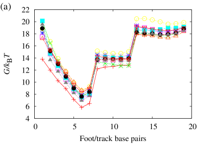
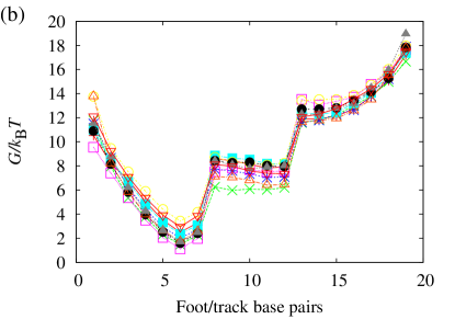
Figure S13: Results of 10 independent estimates of the free-energy profile ($G$) for fuel displacement of the track; (a) without tension and (b) with the track under 14.6 pN of tension. The combination of the ten separate estimates into a single profile for each case is shown in Fig. 10 of the main text. Free energies are given as a function of the number of foot/track base pairs ($\psi_{1}$), subject to the constraint that the fuel is bound to the foot by at least one base pair ($\psi_{2}>0$, $\psi_{3}=3$). Free energies are reported relative a system without bound fuel ($\psi_{2}=0$, $\psi_{3}=0,1,2,3$).

References

- (1) W. Saenger, Principles of Nucleic Acid Structure (Springer-Verlag, New York, 1984).
- (2) P.J. Hagerman, Annu. Rev. Biophys. Biophys. Chem. 17, 265 (1988).
- (3) J.B. Mills, E. Vacano and P.J. Hagerman, J. Mol. Biol. 285, 245 (1999).
- (4) M.C. Murphy, I. Rasnik, W. Chang, T.M. Lohman and T. Ha, Biophys. J. 86, 2530 (2004).
- (5) N.C. Seeman, J. Theor. Biol. 99, 237 (1982).
- (6) N.R. Kallenbach, R.I. Ma and N.C. Seeman, Nature 305, 829 (1983).
- (7) J. Zheng, J.J. Birktoft, Y. Chen, T. Wang, R. Sha, P.E. Constantinou, S.L. Ginell, C. Mao and N.C. Seeman, Nature 461, 74 (2009).
- (8) P.J. Paukstelis, J. Nowakowski, J.J. Birktoft and N.C. Seeman, Chem. Biol. 11, 1119 (2004).
- (9) H. Yan, S. Park, G. Finkelstein, J.H. Reif and T.H. LaBean, Science 301, 1882 (2003).
- (10) E. Winfree, F.R. Liu, L.A. Wenzler and N.C. Seeman, Nature 394, 539 (1998).
- (11) J. Malo, J.C. Mitchell, C. Venien-Bryan, J.R. Harris, H. Wille, D.J. Sherrat and A.J. Turberfield, Angew. Chem. Int. Ed. 44, 3057 (2005).
- (12) F. Zhang, Y. Liu and H. Yan, J. Am. Chem. Soc. 135, 7458 (2013).
- (13) S. Biffi, R. Cerbino, F. Bomboi, E.M. Paraboschi, R. Asselta, F. Sciortino and T. Bellini, Proc. Natl. Acad. Sci. U.S.A. 110, 15633 (2013).
- (14) J. Chen and N.C. Seeman, Nature 350, 631 (1991).
- (15) Y. Zhang and N.C. Seeman, J. Am. Chem. Soc. 116, 1661 (1994).
- (16) R.P. Goodman, I.A.T. Sharp, C.F. Tardin, C.M. Erben, R.M. Berry, C.F. Schmidt and A.J. Turberfield, Science 310, 1661 (2005).
- (17) C.M. Erben, R.P. Goodman and A.J. Turberfield, J. Am. Chem. Soc. 129, 6992 (2007).
- (18) F.F. Andersen, B. Knudsen, C.L.P. Oliveira, R.F. Frohlich, D. Kruger, J. Bungert, M. Agbandje-McKenna, R. McKenna, J. Sissel, C. Veigaard, J. Koch, J.L. Rubinstein, B. Guldbrandtsen, M.S. Hede, G. Karlsson, A.H. Andersen, J.S. Pedersen and B.R. Knudsen, Nucl. Acids Res. 36, 1113 (2008).
- (19) Y. Ke, L.L. Ong, W.M. Shih and P. Yin, Science 338, 1177 (2012).
- (20) B. Wei, M. Dai and P. Yin, Nature 485, 623 (2012).
- (21) P.W.K. Rothemund, Nature 440, 297 (2006).
- (22) S.M. Douglas, H. Dietz, T. Liedl, B. Högberg, F. Graf and W.M. Shih, Nature 459, 414 (2009).
- (23) E.S. Andersen, M. Dong, M.M. Nielsen, K. Jahn, R. Subramani, W. Mamdouh, M.M. Golas, B. Sander, H. Stark, C.L.P. Oliveira, J.S. Pedersen, V. Birkedal, F. Besenbacher, K.V. Gothelf and J. Kjems, Nature 459, 73 (2009).
- (24) H. Dietz, S.M. Douglas and W.M. Shih, Science 325, 725 (2009).
- (25) D. Han, S. Pal, J. Nangreave, Z. Deng, Y. Liu and H. Yan, Science 332, 342 (2011).
- (26) S.Y. Park, A.K.R. Lytton-Jean, B. Lee, S. Weigand, G.C. Schatz and C.A. Mirkin, Nature 451, 553 (2008).
- (27) F.A. Aldaye and H.F. Sleiman, J. Am. Chem. Soc. 129, 13376 (2007).
- (28) J. Zimmermann, M.P. Cebulla, S. Monninghoff and G. von Kiedrowski, Angew. Chem. Int. Ed. 47, 3626 (2008).
- (29) S.F.J. Wickham, J. Bath, Y. Katsuda, M. Endo, K. Hidaka, H. Sugiyama and A.J. Turberfield, Nat. Nanotechnol. 7, 169 (2012).
- (30) B. Yurke and A. Mills, Genetic Programming and Evolvable Machines 4, 111 (2003).
- (31) D. Zhang and E. Winfree, J. Am. Chem. Soc. 131, 17303 (2009).
- (32) N. Srinivas, T.E. Ouldridge, P. Šulc, J. Schaeffer, B. Yurke, A.A. Louis, J.P.K. Doye and E. Winfree, Nucl. Acids Res. 41, 10641 (2013).
- (33) B. Yurke, A.J. Turberfield, A.P. Mills, F.C. Simmel and J. Neumann, Nature 406, 605 (2000).
- (34) H. Yan, X.P. Zhang, Z.Y. Shen and N.C. Seeman, Nature 415, 62 (2002).
- (35) R.P. Goodman, M. Heilemann, S.D. anc C. M. Erben, A.N. Kapanidis and A.J. Turberfield, Nat. Nanotechnol. 3, 93 (2008).
- (36) D. Han, S. Pal, Y. Liu and H. Yan, Nat. Nanotechnol. 5, 712 (2010).
- (37) W.B. Sherman and N.C. Seeman, Nano Lett. (7), 1203 (2004).
- (38) J.S. Shin and N.A. Pierce, J. Am. Chem. Soc. 126, 10834 (2004).
- (39) M. Liu, R. Hou, J. Cheng, I.Y. Loh, S. Sreelatha, J.N. Tey, J. Wei and Z. Wang, ACS Nano 8, 1792 (2014).
- (40) J. Bath and A.J. Turberfield, Nat. Nanotechnol. 2, 275 (2007).
- (41) J. Bath, S.J. Green and A.J. Turberfield, Angew. Chem. Int. Ed. 117, 4432 (2005).
- (42) J. Bath, S.J. Green, K.E. Allan and A.J. Turberfield, Small 5, 1513 (2009).
- (43) S.F.J. Wickham, M. Endo, Y. Katsuda, K. Hidaka, J. Bath, H. Sugiyama and A.J. Turberfield, Nat. Nanotechnol. 6, 166 (2011).
- (44) Y. Tian, Y. He, Y. Chen, P. Yin and C. Mao, Angew. Chem. Int. Ed. 44, 4355 (2005).
- (45) K. Lund, A.J. Manzo, N. Dabby, N. Michelotti, A. Johnson-Buck, J. Nangreave, S. Taylor, R. Pei, M.N. Stojanovic, N.G. Walter, E. Winfree and H. Yan, Nature 465, 206 (2010).
- (46) T.G. Cha, P. J, H. Chen, J. Salgado, X. Li, C. Mao and J.H. Choi, Nat. Nanotechnol. 9, 39 (2014).
- (47) S.J. Green, J. Bath and A.J. Turberfield, Phys. Rev. Lett. 101, 238101 (2008).
- (48) T. Omabegho, R. Sha and N.C. Seeman, Science 324, 67 (2009).
- (49) S. Venkataraman, R.M. Dirks, P.W.K. Rothemund, E. Winfree and N.A. Pierce, Nat. Nanotechnol. 2, 490 (2007).
- (50) R.A. Muscat, J. Bath and A.J. Turberfield, Nano Lett. 11, 982 (2011).
- (51) L.M. Adleman, Science 266, 1021 (1994).
- (52) G. Seelig, D. Soloveichik, D.Y. Zhang and E. Winfree, Science 314, 1585 (2006).
- (53) L. Qian and E. Winfree, Science 332, 1196 (2011).
- (54) Y.J. Chen, N. Dalchau, N. Srinivas, A. Phillips, L. Cardelli, D. Solveichik and G. Seelig, Nat. Nanotechnol. 8, 755 (2013).
- (55) M.J. Berardi, W.M. Shih, S.C. Harrison and J.J. Chou, Nature 476, 109 (2011).
- (56) D.N. Selmi, R.J. Adamson, H. Attrill, A.D. Goddard, A. Watts and A.J. Turberfield, Nano Lett. 11, 657 (2011).
- (57) A. Kuzyk, R. Schreiber, Z. Fan, G. Pardatscher, E.M. Roller, A. Högele, F.C. Simmel, A.O. Govorov and T. Liedl, Nature 483, 311 (2012).
- (58) P.K. Dutta, R. Varghese, J. Nangreave, S. Lin, H. Yan and Y. Liu, J. Am. Chem. Soc. 133, 11985 (2011).
- (59) C.Y. Tseng and G. Zocchi, J. Am. Chem. Soc. 135, 11879 (2013).
- (60) L. Minghui, J. Fu, C. Christian, Y. Yang, N.W. Woodbury, K.V. Gothelf, Y. Liu and H. Yan, Nat. Commun. 4, 2127 (2013).
- (61) J. Fu, M. Liu, Y. Liu, N.W. Woodbury and H. Yan, J. Am. Chem. Soc. 134, 5516 (2012).
- (62) O.I. Wilner, Y. Weizmann, R. Gill, O. Lioubashevski, R. Freeman and I. Willner, Nat. Nanotechnol. 4, 249 (2009).
- (63) J. Fu, Y.R. Yang, A. Johnson-Buck, M. Liu, Y. Liu, N.G. Walter, N.W. Woodbury and H. Yan, Nat. Nanotechnol. 9, 531 (2014).
- (64) T.E. Tomov, R. Tsukanov, M. Liber, R. Masoud, N. Plavner and E. Nir, J. Am. Chem. Soc. 135, 11935 (2013).
- (65) Y. Ke, S. Lindsay, Y. Chang, Y. Liu and H. Yan, Science 319, 180 (2008).
- (66) H. Subramanian, B. Chakraborty, R. Sha and N. Seeman, Nano Lett. 11, 910 (2011).
- (67) E. Pfitzner, C. Wachauf, F. Kilchherr, B. Pelz, W.M. Shih, M. Reif and H. Dietz, Angew. Chem. Int. Ed. 52, 7766 (2013).
- (68) M. Endo, K. Tatsumi, K. Terushima, Y. Katsuda, K. Hidaka, Y. Harada and H. Sugiyama, Angew. Chem. Int. Ed. 124, 8908 (2012).
- (69) N.D. Derr, B.S. Goodman, R. Jungmann, A.E. Lechziner, W.M. Shih and S.L. Reck-Peterson, Science 338, 662 (2012).
- (70) S.M. Douglas, I. Bachelet and G.M. Church, Science 335, 831 (2012).
- (71) R. Crawford, C.M. Erben, J. Periz, L.M. Hall, T. Brown, A.J. Turberfield and A.N. Kapanidis, Angew. Chem. Int. Ed. 52, 2284 (2013).
- (72) X. Liu, Y. Xu, T. Yu, C. Clifford, Y. Liu, H. Yan and Y. Chang, Nano Lett. 12, 4254 (2012).
- (73) J. Li, H. Pei, B. Zhu, L. Liang, M. Wei, Y. He, N. Chen, D. Li, Q. Huang and C. Fan, ACS Nano 5, 8783 (2011).
- (74) V.J. Schüller, S. Heidegger, N. Sandholzer, P.C. Nickels, N.A. Suhartha, S. Endres, C. Bourquin and T. Liedl, ACS Nano 5, 9696 (2011).
- (75) A.S. Walsh, H. Yin, C.M. Erben, M.J.A. Wood and A.J. Turberfield, ACS Nano 5, 5427 (2011).
- (76) H. Lee, A.K.R. Lytton-Jean, Y. Chen, K.T. Love, A.I. Park, E.D. Karagiannis, A. Sehgal, W. Querbes, C.S. Zurenko, M. Jayaraman, C.G. Peng, K. Charisse, A. Borodovsky, M. Manoharan, J.S. Donahoe, J. Truelove, M. Nahrendorf, R. Langer and D.G. Anderson, Nat. Nanotechnol. 7, 389 (2012).
- (77) Q. Mei, X. Wei, F. Su, Y. Liu, C. Youngbull, R. Johnson, S. Lindsay, H. Yan and D. Meldrum, Nano Lett. 11, 1477 (2011).
- (78) S. Surana, D. Bhatia and Y. Krishnan, Methods 64, 94 (2013).
- (79) S.D. Perrault and W.M. Shih, ACS Nano 8, 5132 (2014).
- (80) J. Mikkilä, A.P. Eskelinen, E.H. Niemelä, V. Linko, M.J. Frilander, P. Törmä and M.A. Kostiainen, Nano Lett. 14, 2196 (2014).
- (81) Y. Amir, E. Ben-Ishay, D. Levner, S. Ittah, A. Abu-Horowitz and I. Bachalet, Nat. Nanotechnol. 9, 353 (2014).
- (82) Y. He and D.R. Liu, Nat. Nanotechnol. 5, 778 (2010).
- (83) M.L. McKee, P.J. Milnes, J. Bath, E. Stulz, R.K. O’Reilly and A.J. Turberfield, J. Am. Chem. Soc. 134, 1446 (2012).
- (84) H. Gu, J. Chao, S. Xiao and N.C. Seeman, Nature 465, 202 (2010).
- (85) J.P.J. Sobczak, T.G. Martin, T. Gerling and H. Dietz, Science 338, 1458 (2012).
- (86) C. Myhrvold, M. Dai, P.A. Silver and P. Yin, Nano Lett. 13, 4242 (2013).
- (87) A. Reinhardt and D. Frenkel, Phys. Rev. Lett. 112, 238103 (2014).
- (88) J.M. Arbona, J. Elezgary and J.P. Aimé, Europhys. Lett. 100, 28006 (2012).
- (89) Y. Ke, G. Bellot, N.V. Voigt, E. Fradkov and W.M. Shih, Chem. Sci. 3, 2587 (2012).
- (90) T.G. Martin and H. Dietz, Nat. Commun. 3, 1103 (2012).
- (91) H. Chen, T.W. Weng, M.M.R. an Y. Cui, J. Irudayaraj and J.H. Choi, J. Am. Chem. Soc. 136, 6995 (2014).
- (92) R. Tsukanov, T.E. Tomov, R. Masoud, H. Drory, N. Plavner, M. Liber and E. Nir, J. Phys. Chem. B 117, 11932 (2013).
- (93) A. Johnson-Buck, J. Nangreave, S. Jiang, H. Yan and N.G. Walter, Nano Lett. 13, 2754 (2013).
- (94) M. Teichmann, E. Kopperger and F.C. Simmel, ACS Nano (In Press).
- (95) J. SantaLucia, Jr. and D. Hicks, Annu. Rev. Biophys. Biomol. Struct. 33, 415 (2004).
- (96) R.M. Dirks, J.S. Bois, J.M. Schaeffer, E. Winfree and N.A. Pierce, SIAM Rev. 29, 65 (2007).
- (97) F. Oteri, M. Falconi, G. Chilemi, F.F. Andersen, C.L.P. Oliveira, J.S. Pedersen, B.R. Knudsen and A. Desideri, J. Phys. Chem. C 168, 11519 (2011).
- (98) J. Yoo and A. Aksimentiev, Proc. Natl. Acad. Sci. USA 110, 20099 (2013).
- (99) N.B. Becker and R. Everaers, J. Chem. Phys. 130, 135102 (2009).
- (100) F. Lankaš, O. Gonzalez, L.M. Heffler, G. Stoll, M. Moakher and J.H. Maddocks, Phys. Chem. Chem. Phys. 11, 10565 (2009).
- (101) M. Sayar, B. Avşarolu and A. Kabakçıolu, Phys. Rev. E 81, 041916 (2010).
- (102) A. Savelyev and G.A. Papoian, Proc. Natl. Acad. Sci. U.S.A 107, 20340 (2010).
- (103) P.D. Dans, A. Zeida, M.R. Machado and S. Pantano, J. Chem. Theory Comput. 6, 1711 (2010).
- (104) A. Morriss-Andrews, J. Rottler and S.S. Plotkin, J. Chem. Phys. 132, 035105 (2010).
- (105) I.P. Kikot, A.V. Savin, E.A. Zubova, M.A. Mazo, E.B. Gusarova, L.I. Manevitch and A.V. Onufriev, Biophysics 56, 387 (2011).
- (106) A.V. Savin, M.A. Mazo, I.P. Kikot, L.I. Manevitch and A.V. Onufriev, Phys. Rev. B 83, 245406 (2011).
- (107) O. Gonzalez, D. Petkevičiutė and J.H. Maddocks, J. Chem. Phys. 138, 055102 (2013).
- (108) Y. He, M. Maciejczyk, S. Ołdziej, H.A. Scheraga and A. Liwo, Phys. Rev. Lett. 110, 098101 (2013).
- (109) N.A. Kovaleva, I.P. Kikot, M.A. Mazo and E.A. Zubova, arXiv:1401.2770 (2014).
- (110) N.B. Becker and R. Everaers, Phys. Rev. E 76, 021923 (2007).
- (111) C. Maffeo, T.T.M. Ngo, T. Ha and A. Aksimentiev, J. Chem. Theory Comput. 10, 2891 (2013).
- (112) N. Korolev, D. Luo, A.P. Lyubartsev and L. Nordenskiöld, Polymers 6, 1655 (2014).
- (113) A. Naômé, A. Laasksonen and D.P. Vercauteren, J. Chem. Theory Comput. 10, 3541 (2014).
- (114) W.K. Olson, A.A. Gorin, X.J. Lu, L.M. Hock and V.B. Zhurkin, Proc. Natl. Acad. Sci. U.S.A. 95, 11163 (1998).
- (115) F. Trovato and V. Tozzini, J. Phys. Chem. B 112, 13197 (2008).
- (116) M.E. Johnson, T. Head-Gordon and A.A. Louis, J. Chem. Phys. 126, 144509 (2007).
- (117) C.W. Hsu, M. Fyta, G. Lakatos, S. Melchionha and E. Kaxiras, J. Chem. Phys. 137, 105102 (2012).
- (118) K. Drukker, G. Wu and G.C. Schatz, J. Chem. Phys. 114, 579 (2001).
- (119) M. Sales-Pardo, R. Guimera, A.A. Moreira, J. Widom and L. Amaral, Phys. Rev. E 71, 051902 (2005).
- (120) F.W. Starr and F. Sciortino, J.Phys.: Condens. Matter 18, 347 (2006).
- (121) N.B. Tito and J.M. Stubbs, Chem. Phys. Lett. 485, 354 (2010).
- (122) T.A. Knotts, IV, N. Rathore, D. Schwartz and J.J. de Pablo, J. Chem. Phys. 126 (084901) (2007).
- (123) E.J. Sambriski, D.C. Schwartz and J.J. de Pablo, Biophys. J. 96, 1675 (2009).
- (124) D.M. Hinckley, G.S. Freeman, J.K. Whitmer and J.J. de Pablo, J. Chem. Phys. 139, 144903 (2013).
- (125) C. Svaneborg, Comput. Phys. Commun. 183, 1793 (2012).
- (126) M. Kenward and K.D. Dorfman, J. Chem. Phys. 130, 095101 (2009).
- (127) M.C. Linak, R. Tourdot and K.D. Dorfman, J. Chem. Phys. 135, 205120 (2011).
- (128) J.C. Araque, A.Z. Panagiotopoulos and M.A. Robert, J. Chem. Phys. 134, 165103 (2011).
- (129) S. Niewieczerzał and M. Cieplak, J. Phys.: Condens. Matter 21, 474221 (2009).
- (130) L.E. Edens, J.A. Brozik and D.J. Keller, J. Phys. Chem. B 116, 14735 (2012).
- (131) A.K. Dasanna, N. Destainville, J. Palmeri and M. Manghi, Phys. Rev. E 87, 052703 (2013).
- (132) T. Cragnolini, P. Derreumaux and S. Pasquali, J. Phys. Chem. B 117, 8047 (2013).
- (133) K. Doi, T. Haga, H. Shintaku and S. Kawano, Phil. Trans. R. Soc. A 368, 2615 (2010).
- (134) S.P. Mielke, N. Gronbech-Jensen, V.V. Krishnan, W.H. Fink and C.J. Benham, J. Chem. Phys. 123, 124911 (2005).
- (135) C. Knorowski, S. Burleigh and A. Travesset, Phys. Rev. Lett. 106, 215501 (2011).
- (136) J.M. Arbona, J.P. Aimé and J. Elezgaray, Phys. Rev. E 86, 051912 (2012).
- (137) T.E. Ouldridge, A.A. Louis and J.P.K. Doye, J. Chem. Phys. 134, 085101 (2011).
- (138) T.E. Ouldridge, Ph.D. thesis, University of Oxford 2011 [Published as a book by Springer, Heidelberg, 2012].
- (139) P. Šulc, F. Romano, T.E. Ouldridge, L. Rovigatti, J.P.K. Doye and A.A. Louis, J. Chem. Phys. 137, 135101 (2012).
- (140) J.H. Allen, E.T. Schoch and J.M. Stubbs, J. Phys. Chem. B 115, 1720 (2011).
- (141) T.R. Prytkova, I. Eryazici, B. Stepp, S. Nguyen and G.C. Schatz, J. Phys. Chem. B 114, 2627 (2010).
- (142) M.J. Hoefert, E.J. Sambriski and J.J. de Pablo, Soft Matter 7, 560 (2011).
- (143) T.J. Schmitt, B. Rogers and T.A. Knotts IV, J. Chem. Phys. 138, 035102 (2013).
- (144) D. Hinckley, J.P. Lequieu and J.J. de Pablo, J. Chem. Phys. 141, 035102 (2014).
- (145) F.B. Bombelli, F. Gambinossi, M. Lagi, D. Berti, G. Caminati, T. Brown, F. Sciortino, B. Norden and P. Baglioni, J. Phys. Chem. B 112, 15283 (2008).
- (146) J.M. Arbona, J.P. Aimé and J. Elezgaray, J. Chem. Phys. 136, 065102 (2012).
- (147) C. Svaneborg, H. Fellermann and S. Rasmussen, in DNA Computing and Molecular Programming, edited by D. Stefanovic and A. J. Turberfield (, , 2012), Vol. 7433, pp. 123–134.
- (148) T.E. Ouldridge, I.G. Johnston, A.A. Louis and J.P.K. Doye, J. Chem. Phys. 130, 065101 (2009).
- (149) C. Svaneborg, H. Fellerman and S. Rasmussen, arxiv1210.6156 (2012).
- (150) T.I. Li, R. Sknepnek, R.J. Macfarlane, C.A. Mirkin and M.O. de la Cruz, Nano Lett. 12, 2509 (2012).
- (151) C. Hyeon and D. Thirumalai, Proc. Natl. Acad. Sci. U.S.A. 102, 6789 (2005).
- (152) A. Cao and S.J. Chen, Nucl. Acids Res. 34, 2634 (2006).
- (153) D. Jost and R. Everaers, J. Chem. Phys. 132, 095101 (2010).
- (154) F. Ding, S. Sharma, P. Chalasani, V.V. Demidov, N.E. Broude and N.V. Dokholyan, RNA 14, 1164 (2008).
- (155) S. Pasquali and P. Derreumaux, The Journal of Physical Chemistry B 114, 11957 (2010).
- (156) A. Dickson, M. Maienschein-Cline, A. Tovo-Dwyer, J.R. Hammond and A.R. Dinner, J. Chem. Theory Comput. 7, 2710 (2011).
- (157) N.A. Denesyuk and D. Thirumalai, J. Phys. Chem. B 117, 4901 (2013).
- (158) M.A. Jonikas, R.J. Radmer, A. Laederach, R. Das, S. Pearlman, D. Herschlag and R.B. Altman, RNA 15, 189 (2009).
- (159) R. Das and D. Baker, Proc. Natl. Acad. Sci. U.S.A 104, 14664 (2009).
- (160) M. Paliy, R. Melnik and B.A. Shapiro, Phys. Biol. 7, 036001 (2010).
- (161) Z. Xia, D.R. Bell, Y. Shi and P. Ren, J. Phys. Chem. B 117, 3135 (2013).
- (162) S. Whitelam, E.H. Feng, M.F. Hagan and P.L. Geissler, Soft Matter 5, 1251 (2009).
- (163) R.L. Davidchack, R. Handel and M.V. Tretyakov, J. Chem. Phys. 130, 234101 (2009).
- (164) J. Russo, P. Tartaglia and F. Sciortino, J, Chem. Phys. 131, 014504 (2009).
- (165) G.M. Torrie and J.P. Valleau, J. Comp. Phys. 23, 187 (1977).
- (166) R.J. Allen, P.B. Warren and P.R. ten Wolde, Phys. Rev. Lett. 94, 018104 (2005).
- (167) R.J. Allen, C. Valeriani and P.R. ten Wolde, J. Phys.: Condens. Matter 21, 463102 (2009).
- (168) Q. Wang and B.M. Pettitt, Biophys. J. 106, 1182 (2014).
- (169) T.E. Ouldridge, J. Chem. Phys. 137, 144105 (2012).
- (170) R.R.F. Machinek, T.E. Ouldridge, N.E.C. Haley, J. Bath and A.J. Turberfield, Nat. Commun. In press. doi:NCOMMS6324
- (171) A.J. Genot, D.Y. Zhang, J. Bath and A.J. Turberfield, J. Am. Chem. Soc. 133, 2177 (2011).
- (172) D.Y. Zhang, S.X. Chen and P. Yin, Nat. Chem. 4, 208 (2012).
- (173) Y.S. Jiang, S. Bhadra, B. Li and A.D. Ellington, Angew. Chem. Int. Ed. 126, 1876 (2014).
- (174) Q. Li, G. Luan, Q. Guo and J. Liang, Nucl. Acids Res. 30, e5 (2002).
- (175) D.Y. Zhang, S.X. Chen and Y. Peng, Nat. Chem. 4, 208 (2012).
- (176) S.X. Chen, D.Y. Zhang and G. Seelig, Nat. Chem. 5, 782 (2013).
- (177) P. Šulc, T.E. Ouldridge, F. Romano, J.P.K. Doye and A.A. Louis, Nat. Comput. pp. 1–13 (2013).
- (178) T.E. Ouldridge, R.L. Hoare, A.A. Louis, J.P.K. Doye, J. Bath and A.J. Turberfield, ACS Nano 7, 2479 (2013).
- (179) H. Qu, Y. Wang, C.Y. Tseng and G. Zocchi, Phys. Rev. X 1, 021008 (2011).
- (180) J. Wang, H. Qu and G. Zocchi, Phys. Rev. E 88, 032712 (2013).
- (181) Y. Li, C. Zhang, C. Tian and C. Mao, Org. Biomol. Chem. 12, 2543 (2014).
- (182) J.R. Sikora, B. Rauzan, R. Stegemann and A. Deckert, J. Phys. Chem. B 117, 8966 (2013).
- (183) T.E. Ouldridge, P. Šulc, F. Romano, J.P.K. Doye and A.A. Louis, Nucl. Acids Res. 41, 8886 (2013).
- (184) P.A. Wiggins, T. van der Heijden, F. Moreno-Herrero, A. Spakowitz, R. Phillips, J. Widom, C. Dekker and P.C. Nelson, Nat. Nanotechnol. 1, 137 (2006).
- (185) R. Vafabakhsh and T. Ha, Science 337, 1097 (2012).
- (186) A. Vologodskii and M.D. Frank-Kamenetskii, Nucl. Acids Res. 41, 6785 (2013).
- (187) A.K. Mazur and M. Maaloum, Phys. Rev. Lett. 112, 068104 (2014).
- (188) J.P.K. Doye, T.E. Ouldridge, A.A. Louis, F. Romano, P. Šulc, C. Matek, B. Snodin, L. Rovigatti, J.S. Schreck, R.M. Harrison and W.P.J. Smith, Phys. Chem. Chem. Phys. 15, 20395 (2013).
- (189) L. Rovigatti, F. Smallenburg, F. Romano and F. Sciortino, ACS Nano 8, 3567 (2014).
- (190) L. Rovigatti, F. Bomboi and F. Sciortino, J. Chem. Phys. 140, 154903 (2014).
- (191) P. Šulc, F. Romano, T.E. Ouldridge, J.P.K. Doye and A.A. Louis, J. Chem. Phys. 140, 235102 (2014).
- (192) J. Schaeffer, Ph.D. thesis, California Institute of Technology 2013.
- (193) A. Phillips and L. Cardelli, J. R. Soc. Interface 6, S419 (2009).
- (194) S. Whitelam and P. L. Geissler, J. Chem. Phys. 127, 154101 (2007).
- (195) S. Kumar, J. M. Rosenberg, D. Bouzida, R. H. Swendsen, and P. A. Kollman, J. Comput. Chem. 13, 1011 (1992).
- (196) J. Lapham, J. P. Rife, P. B. Moore, and D. M. Crothers, J. NMR 10, 252 (1997).