IFT-UAM/CSIC-14-113
                                                                                                                         FTUAM-14-45
Electroweak chiral Lagrangian with a light Higgs
and $\gamma\gamma\to Z_{L}Z_{L},W_{L}^{+}W_{L}^{-}$ scattering at one loop

Abstract

In these proceedings we provide a brief summary of the findings of a previous article where we have studied the photon-photon scattering into longitudinal weak bosons within the context of the electroweak chiral Lagrangian with a light Higgs, a low-energy effective field theory including a Higgs-like scalar singlet and where the electroweak would-be Goldstone bosons are non-linearly realized. We consider the relevant Lagrangian up to next-to-leading order in the chiral counting, which is explained in some detail here. We find that these amplitudes are ultraviolet finite and the relevant combinations of next-to-leading parameters ($c_{\gamma}$ and $a_{1}-a_{2}+a_{3}$) do not get renormalized. We propose the joined analysis of $\gamma\gamma$–scattering and other photon related observables ($\Gamma(h\to\gamma\gamma)$, $S$–parameter and the $\gamma^{*}\to W^{+}_{L}W^{-}_{L}$ and $\gamma^{*}\to h\gamma$ electromagnetic form-factors) in order to separate and determine each chiral parameter. Moreover, the correlations between observables provided by the NLO computations would lead to more stringent bounds on the new physics that is parametrized by means of this effective Lagrangian. We also show an explicit computation of the $\gamma\gamma$–scattering up to next-to-leading order in the $SO(5)/SO(4)$ minimally composite Higgs model.

1 $\gamma\gamma$–scattering as a probe into new physics

Two years ago the Large Hadron Collider (LHC) discovered a new particle, most likely a scalar, with mass $m_{h}\approx 125$ GeV [1] and couplings so far compatible with what one would expect for the Standard Model (SM) Higgs boson. We are therefore in a scenario with small deviations from the SM and, apparently, a large mass gap (as no new particle has shown up below the TeV). Thus, the effective field theory (EFT) framework seems to be the most convenient one to confront current experimental    data    and    to  explore     possible   beyond

Standard Model (BSM) effects in the electroweak (EW) sector.

In these proceedings we discuss some of the findings in a previous work [2]. Therein we studied the processes $\gamma\gamma\to Z_{L}Z_{L}$ and $\gamma\gamma\to W_{L}^{+}W_{L}^{-}$ in the context of a general EW low-energy effective field theory (EFT), which we will denote as Electroweak Chiral Lagrangian with a light Higgs (ECLh), with the EW would-be Goldstone bosons (WBGBs) denoted here by $w^{a}$ and non-linearly realized. In addition to be more general, this non-linear representation seems to be more appropriate in the case of strong interactions in the EW sector, as it is the case in Quantum Chromodynamics [3, 4]. The three would-be Goldstone bosons $w^{a}$ from the spontaneous EW symmetry breaking are parametrized through a unitary matrix $U$ that takes values in the $SU(2)_{L}\times SU(2)_{R}/SU(2)_{L+R}$ coset. 

The Higgs boson does not enter in the SM at tree-level in these $\gamma\gamma\to V_{L}V_{L}$ ($V=Z,W$) processes (where in addition ${\mathcal{M}(\gamma\gamma\to Z_{L}Z_{L})^{\rm tree}_{\rm SM}=0}$ [6]). Nevertheless, one can search for new physics by studying the one-loop corrections [2], which are sensitive to deviations from the SM in the Higgs boson couplings. Our analysis [2] is performed in the Landau gauge and making use of the Equivalence Theorem (Eq.Th.) [7],

$$\mathcal{M}(\gamma\gamma\to W_{L}^{a}W_{L}^{b}) \simeq \,-\,\mathcal{M}(\gamma\gamma\to w^{a}w^{b})\,,$$ (1)

valid in the energy regime $m_{W}^{2},m_{Z}^{2}\ll s$. The EW gauge boson masses $m_{W,Z}$ are then neglected in our computation. Furthermore, since experimentally $m_{h}\sim m_{W,Z}$ we also neglect $m_{h}$ in our calculation. In summary, the applicability range in [2] is

$$m_{h}^{2}\,\sim\,m_{W}^{2},\,m_{Z}^{2}\quad\stackrel{{\scriptstyle\rm Eq.Th.}}{{\ll}}\quad s,\,t,\,u\quad\stackrel{{\scriptstyle\rm EFT}}{{\ll}}\quad\Lambda_{\rm ECLh}^{2}\,,$$ (2)

with the upper limit given by the EFT cut-off $\Lambda_{\rm ECLh}$, expected to be of the order of $4\pi{\rm v}\simeq 3$ TeV or the mass of possible heavy BSM particles, where ${\rm v}=246$ GeV denotes the SM Higgs vacuum expectation value.

Although our derivation is general and does not assume any particular underlying BSM theory, it is obviously inspired by models where the Higgs is another (pseudo) Nambu-Goldstone boson (NGB). Indeed, in the final part of these proceedings we provide an explicit example for the $SO(5)/SO(4)$ Minimally Composite Higgs Model (MCHM) [8].

2 ECLh up to next-to-leading order

The WBGBs are described by a matrix field $U$ that takes values in the $SU(2)_{L}\times SU(2)_{R}/SU(2)_{L+R}$ coset, and transforms as $U\to LUR^{\dagger}$ [9, 10]. The basic building blocks employed to construct the relevant ECLh Lagrangian for our analysis are [2, 9, 10]

$$D_{\mu}U=\partial_{\mu}U+i\hat{W}_{\mu}U-iU\hat{B}_{\mu}\,,\;V_{\mu}=(D_{\mu}U)U^{\dagger}\,,\;$$

$$\hat{W}_{\mu\nu}=\partial_{\mu}\hat{W}_{\nu}-\partial_{\nu}\hat{W}_{\mu}+i[\hat{W}_{\mu},\hat{W}_{\nu}],\quad\hat{B}_{\mu\nu}=\partial_{\mu}\hat{B}_{\nu}-\partial_{\nu}\hat{B}_{\mu},$$

$$\hat{W}_{\mu}=gW_{\mu}^{a}\tau^{a}/2,\;\hat{B}_{\mu}=g^{\prime}\,B_{\mu}\tau^{3}/2\,.$$ (3)

with well-defined transformation properties [2, 10]. The Higgs field $h$ is a singlet in the ECLh and enters in the Lagrangian operators via polynomials or their partial derivatives [11, 12]. These building blocks are employed to construct ECLh operators with CP, Lorentz and $SU(2)_{L}\times U(1)_{Y}$ gauge invariance.

We consider the following scaling in powers of momentum $p$,

$$\partial_{\mu}\,,m_{W}\,,m_{Z},\,m_{h}\sim{\cal O}(p)\,,\quad g,\,g^{\prime},\,e\sim{\cal O}(p/{\rm v})\,,$$ (4)

and the counting for the tensors above [2, 13, 14],

$$D_{\mu}U,\;V_{\mu}\sim{\cal O}(p),\quad\hat{W}_{\mu\nu},\;\hat{B}_{\mu\nu}\sim{\cal O}(p^{2})\,.$$ (5)

Within the approximations of our analysis [2], the relevant ECLh operators for $\gamma\gamma\to w^{a}w^{b}$ at leading order (LO) –${\cal O}(p^{2})$– and next-to-leading order (NLO) in the chiral counting –${\cal O}(p^{4})$– are [2, 10]

$$\mathcal{L}_{2}=-\frac{\displaystyle 1}{\displaystyle 2g^{2}}{\rm Tr}(\hat{W}_{\mu\nu}\hat{W}^{\mu\nu})-\frac{\displaystyle 1}{\displaystyle 2g^{{}^{\prime}2}}{\rm Tr}(\hat{B}_{\mu\nu}\hat{B}^{\mu\nu})$$

$$+\frac{\displaystyle{\rm v}^{2}}{\displaystyle 4}\left[1+2a\frac{\displaystyle h}{\displaystyle{\rm v}}+b\frac{\displaystyle h^{2}}{\displaystyle{\rm v}^{2}}\right]{\rm Tr}(D^{\mu}U^{\dagger}D_{\mu}U)+\frac{\displaystyle 1}{\displaystyle 2}\partial^{\mu}h\,\partial_{\mu}h+\dots\,,$$

$$\mathcal{L}_{4}=a_{1}{\rm Tr}(U\hat{B}_{\mu\nu}U^{\dagger}\hat{W}^{\mu\nu})+ia_{2}{\rm Tr}(U\hat{B}_{\mu\nu}U^{\dagger}[V^{\mu},V^{\nu}])$$

$$-ia_{3}{\rm Tr}(\hat{W}_{\mu\nu}[V^{\mu},V^{\nu}])-\frac{\displaystyle c_{\gamma}}{\displaystyle 2}\frac{\displaystyle h}{\displaystyle{\rm v}}e^{2}A_{\mu\nu}A^{\mu\nu}\,+\,...$$ (6)

where one has the photon field strength $A_{\mu\nu}=\partial_{\mu}A_{\nu}-\partial_{\nu}A_{\mu}$ and the dots stand for operators not relevant within our approximations for the $\gamma\gamma$-scattering [2].

The classification of the chiral order in the previous Lagrangian (6) provides a consistent perturbative expansion as we show now in more detail. First, we denote as ${\cal O}(p^{d})$ any operator of the generic form

$$\mathcal{L}_{d} = \sum_{k}f_{k}^{(d)}p^{d}\left(\frac{\chi}{{\rm v}}\right)^{k}\,,$$ (7)

with $\chi$ any bosonic field ($h$, $w^{a}$, $W^{a}_{\mu}$, $B_{\mu}$), $p$ refers to derivatives $\partial$ or light masses $m_{h,W,Z}$ acting appropriately on the fields, and $f_{k}^{(d)}$ are the corresponding couplings of the operator ($f_{k}^{(2)}\sim{\rm v}^{2}$, $f_{k}^{(4)}\sim a_{i},c_{\gamma}...$). Let us now consider an arbitrary diagram with $L$ loops, $I$ internal boson propagators and $N_{d}$ vertices from $\mathcal{L}_{d}$ (with total number of vertices $V=\sum_{d}N_{d}$). Following Weinberg’s dimensional arguments [3], it is not difficult to see that in dimensional regularization this amplitude will scale with $p$ like [2, 3, 13]

$$\mathcal{M}\,\,\sim\,\,\displaystyle{\int}(d^{4}p)^{L}\,\frac{\displaystyle 1}{\displaystyle(p^{2})^{I}}\,\prod_{d}(p^{d})^{N_{d}}\,\,\sim\,\,p^{4L-2I+\sum_{d}dN_{d}}$$

$$\sim\,\,\,p^{2+2L+\sum_{d}(d-2)N_{d}}\,,$$ (8)

where we have used the topological identity $I=L+V-1$ in the last line. Finally, keeping track of the constant factors with powers of $(16\pi^{2})^{-1}$ (from loops) and ${\rm v}$ (coming with every field $\chi$ in (7)), and the coupling constants $f_{k}^{(d)}$ (from every vertex $\mathcal{L}_{d}$), it is not difficult to complete the previous formula into [2]

$$\mathcal{M}\,\,\sim\,\,\left(\frac{\displaystyle p^{2}}{\displaystyle{\rm v}^{N_{E}-2}}\right)\,\left(\frac{\displaystyle p^{2}}{\displaystyle 16\pi^{2}{\rm v}^{2}}\right)^{L}\,\prod_{d}\left(\frac{\displaystyle f_{k}^{(d)}p^{d-2}}{\displaystyle{\rm v}^{2}}\right)^{N_{d}}\,,$$ (9)

with $N_{E}$ the number of external boson legs, which shows up in the final expression after counting the total number of fields from all the $\mathcal{L}_{d}$ vertices, and hence the total number of powers of ${\rm v}^{-1}$: the diagram carries then the factor $({\rm v}^{-1})^{2I+N_{E}}=({\rm v}^{-1})^{N_{E}-2+2L+\sum_{d}2N_{d}}$, as shown above.

The various possible contributions to the amplitude of a given process can be then sorted in the form

$$\mathcal{M} = \underbrace{\mathcal{M}_{{\cal O}(p^{2})}}_{{\rm\bf LO}}\,\,+\,\,\underbrace{\mathcal{M}_{{\cal O}(p^{4})}}_{{\rm\bf NLO}}\,\,+\,\,...$$ (10)

Observing Eq. (9) one can see that higher orders in the chiral expansion can be reached by either adding more loops $L$ to the diagram or vertices of “chiral dimension” $d\geq 4$. Notice that adding vertices from $\mathcal{L}_{2}$ does not modify the scaling of the diagram with $p$, as far as the number of loops $L$ remains the same. At LO, one needs to consider only the tree-level diagrams made out of $\mathcal{L}_{2}$ vertices ($L=0$, $N_{2}$ arbitrary, $N_{d\geq 4}=0$); at NLO, one needs to compute the one-loop diagrams with $\mathcal{L}_{2}$ vertices ($L=1$, $N_{2}$ arbitrary, $N_{d\geq 4}=0$) and tree-level diagrams with one vertex from $\mathcal{L}_{4}$ and any number of vertices from $\mathcal{L}_{2}$ ($L=0$, $N_{2}$ arbitrary, $N_{4}=1$, $N_{d\geq 6}=0$); the procedure is analogous for higher chiral orders.

In our particular computation of $\mathcal{M}(\gamma\gamma\to w^{a}w^{b})$ up to NLO, the contributions we find are sorted out in the form [2]

$$\mathcal{M}\,=\,\underbrace{{\cal O}(e^{2})}_{\rm LO,\,tree}\,+\,\underbrace{{\cal O}\left(e^{2}\frac{\displaystyle p^{2}}{\displaystyle 16\pi^{2}{\rm v}^{2}}\right)}_{\rm NLO,\,1-loop}\,+\,\underbrace{{\cal O}\left(e^{2}\frac{\displaystyle a_{i}p^{2}}{\displaystyle{\rm v}^{2}}\right)}_{\rm NLO,\,tree}\,,$$ (11)

where $e\sim{\cal O}(p/{\rm v})$ and $a_{i}$ stands for a general $\mathcal{L}_{4}$ coupling. These three types of contributions can be better understood through the detailed analysis of the examples in Fig. 1, three of the many diagrams entering in $\gamma\gamma\to w^{+}w^{-}$ up to NLO [2]:

• a) The tree-level amplitude in Fig. 1.a with vertices from $\mathcal{L}_{2}$ scales like [2]

  $$\mathcal{M}_{{\rm\bf a}}\sim\,(e\,p)\,\frac{\displaystyle 1}{\displaystyle p^{2}}\,(e\,p)\,\sim\,e^{2}\,,$$

  with each $\gamma w^{+}w^{-}$ vertex scaling like $e\,p$ and the intermediate propagator like $p^{-2}$.

• b) The one-loop amplitude in Fig. 1.b with vertices from $\mathcal{L}_{2}$ scales like [2]

  $$\mathcal{M}_{{\rm\bf b}}\sim\int\frac{\displaystyle d^{4}p}{\displaystyle(2\pi)^{d}}\,\,(e\,p)^{2}\,\left(\frac{p^{2}}{{\rm v}}\right)^{2}\,\frac{\displaystyle 1}{\displaystyle(p^{2})^{4}}\,\sim\,e^{2}\,\frac{\displaystyle p^{2}}{\displaystyle 16\pi^{2}{\rm v}^{2}}\,,$$

  with each $\gamma w^{+}w^{-}$ vertex scaling like $e\,p$, each $hw^{+}w^{-}$ vertex like $p^{2}/{\rm v}$ and each internal propagator like $p^{-2}$. This amplitude actually comes together with logarithms of the energy and ultraviolet (UV) divergences.

• c) The tree-level amplitude in Fig. 1.c with one vertex from $\mathcal{L}_{4}$ and vertices from $\mathcal{L}_{2}$ scales like [2]

  $$\mathcal{M}_{{\rm\bf c}}\sim\,\,\left(\frac{\displaystyle c_{\gamma}\,e^{2}p^{2}}{\displaystyle{\rm v}}\right)\,\frac{\displaystyle 1}{\displaystyle p^{2}}\,\left(\frac{\displaystyle p^{2}}{\displaystyle{\rm v}}\right)\,\sim\,e^{2}\,\frac{\displaystyle c_{\gamma}p^{2}}{\displaystyle{\rm v}^{2}}\,,$$

  with the $\gamma\gamma h$ vertex from $\mathcal{L}_{4}$ scaling like  $c_{\gamma}e^{2}p^{2}/{\rm v}$, the $hw^{+}w^{-}$ vertex like $p^{2}/{\rm v}$ and the intermediate Higgs propagator like $p^{-2}$. In general, the cancelation of the UV divergences in the one-loop NLO diagrams will require the renormalization of the $\mathcal{L}_{4}$ couplings, e.g., $c_{\gamma}^{r}=c_{\gamma}+\delta c_{\gamma}$, $a_{i}^{r}=a_{i}+\delta a_{i}$.

\psfrag{X}{$\gamma$}\includegraphics[scale={0.35}]{diagrams2.eps}

Figure 1: Examples of contributing diagrams to $\gamma\gamma\to w^{+}w^{-}$. a) LO diagram ($L=0$ with only $\mathcal{L}_{2}$ vertices); b) NLO loop diagram ($L=1$ with only $\mathcal{L}_{2}$ vertices); c) NLO tree-level diagram ($L=0$ with one vertex from $\mathcal{L}_{4}$ and any number of $\mathcal{L}_{2}$ vertices). The arrow in the charged $w$ lines indicates the electric charge flow. All the vertices are from $\mathcal{L}_{2}$ but for the gray square in c), which comes from $\mathcal{L}_{4}$.

The $\mathcal{M}(\gamma(k_{1},\epsilon_{1})\gamma(k_{2},\epsilon_{2})\to w^{a}(p_{1})w^{b}(p_{2}))$ amplitudes, with $w^{a}w^{b}=zz,w^{+}w^{-}$, have the Lorentz decomposition [2, 15, 16]

$$\mathcal{M}=ie^{2}(\epsilon_{1}^{\mu}\epsilon_{2}^{\nu}T_{\mu\nu}^{(1)})A(s,t,u)+ie^{2}(\epsilon_{1}^{\mu}\epsilon_{2}^{\nu}T_{\mu\nu}^{(2)})B(s,t,u),$$ (12)

written in terms of the two independent Lorentz structures $T_{\mu\nu}^{(1)}\sim{\cal O}(p^{2})$ and $T_{\mu\nu}^{(2)}\sim{\cal O}(p^{4})$ involving the external momenta,

$$(\epsilon_{1}^{\mu}\epsilon_{2}^{\nu}T^{(1)}_{\mu\nu})=\frac{s}{2}(\epsilon_{1}\epsilon_{2})-(\epsilon_{1}k_{2})(\epsilon_{2}k_{1}),$$ (13)

$$(\epsilon_{1}^{\mu}\epsilon_{2}^{\nu}T^{(2)}_{\mu\nu})=2s(\epsilon_{1}\Delta)(\epsilon_{2}\Delta)-(t-u)^{2}(\epsilon_{1}\epsilon_{2})$$

$$\hskip 28.45274pt-2(t-u)[(\epsilon_{1}\Delta)(\epsilon_{2}k_{1})-(\epsilon_{1}k_{2})(\epsilon_{2}\Delta)]\,,$$

with $\Delta^{\mu}\equiv p_{1}^{\mu}-p_{2}^{\mu}$. The Mandelstam variables are defined as $s=(p_{1}+p_{2})^{2}$, $t=(k_{1}-p_{1})^{2}$ and $u=(k_{1}-p_{2})^{2}$ and the $\epsilon_{i}$’s are the polarization vectors of the initial photons. At LO and NLO we find for the neutral channel [2],

$$A(\gamma\gamma\to zz)_{\rm LO}=B(\gamma\gamma\to zz)_{\rm LO}=B(\gamma\gamma\to zz)_{\rm NLO}=0\,,$$

$$A(\gamma\gamma\to zz)_{\rm NLO}=\frac{\displaystyle 2ac_{\gamma}^{r}}{\displaystyle{\rm v}^{2}}+\frac{\displaystyle(a^{2}-1)}{\displaystyle 4\pi^{2}{\rm v}^{2}}\,,$$ (14)

and for the charged one [2]

$$A(\gamma\gamma\to w^{+}w^{-})_{\rm LO}=2sB(\gamma\gamma\to w^{+}w^{-})_{\rm LO}=-\frac{\displaystyle 1}{\displaystyle t}-\frac{\displaystyle 1}{\displaystyle u},$$

$$A(\gamma\gamma\to w^{+}w^{-})_{\rm NLO}=\frac{\displaystyle 2ac_{\gamma}^{r}}{\displaystyle{\rm v}^{2}}+\frac{\displaystyle 8(a_{1}^{r}-a_{2}^{r}+a_{3}^{r})}{\displaystyle{\rm v}^{2}}+\frac{\displaystyle(a^{2}-1)}{\displaystyle 8\pi^{2}{\rm v}^{2}},$$

$$B(\gamma\gamma\to w^{+}w^{-})_{\rm NLO}=0\,.$$ (15)

The term with $c_{\gamma}^{r}$ comes from the Higgs tree-level exchange in the $s$–channel, the term proportional to $(a^{2}-1)$ comes from the one-loop diagrams with $\mathcal{L}_{2}$ vertices, and the Higgsless operators in (6) yield the tree-level contribution to $\gamma\gamma\to w^{+}w^{-}$ proportional to $(a_{1}-a_{2}+a_{3})$. Independent diagrams are in general UV divergent and have complicated logarithmic and Lorentz structure.  However, in dimensional regularization, when all the different contributions (10 and 39 loop diagrams for the neutral and charged channels, respectively) are put together the final one-loop amplitude turns out to be UV finite and free of logs in the limits considered in our analysis [2], both in $\gamma\gamma\to zz$ and $\gamma\gamma\to w^{+}w^{-}$. Therefore the combinations of NLO couplings $c_{\gamma}$ and $(a_{1}-a_{2}+a_{3})$ which enter here do not need to be renormalized: $a_{1}^{r}-a_{2}^{r}+a_{3}^{r}=a_{1}-a_{2}+a_{3}$ (like in the Higgsless case [15, 16]) and $c^{r}_{\gamma}=c_{\gamma}$ are renormalization group invariant [2]. All the UV divergences and renormalizations occur at ${\cal O}(p^{4})$ and the $\mathcal{L}_{2}$ couplings (like $a$, for instance) do not get renormalized within the approximations considered in this work [2].

	Relevant combinations
Observables	of parameters
	from $\mathcal{L}_{2}$	from $\mathcal{L}_{4}$
$\mathcal{M}(\gamma\gamma\to zz)$	$a$	$c_{\gamma}^{r}$
$\mathcal{M}(\gamma\gamma\to w^{+}w^{-})$	$a$	$(a_{1}^{r}-a_{2}^{r}+a_{3}^{r}),\,c_{\gamma}^{r}$
$\Gamma(h\to\gamma\gamma)$	$a$	$c_{\gamma}^{r}$
$S$–parameter	$a$	$a_{1}^{r}$
$\mathcal{F}_{\gamma^{*}ww}$	$a$	$(a_{2}^{r}-a_{3}^{r})$
$\mathcal{F}_{\gamma^{*}\gamma h}$	–	$c_{\gamma}^{r}$

Table 1: Set of observables studied in Ref. [2] and their corresponding relevant combinations of chiral parameters.

	ECLh	ECL
		(Higgsless)
$\Gamma_{a_{1}-a_{2}+a_{3}}$	$0$	0
$\Gamma_{c_{\gamma}}$	$0$	-
$\Gamma_{a_{1}}$	$-\frac{1}{6}(1-a^{2})$	$-\frac{1}{6}$
$\Gamma_{a_{2}-a_{3}}$	$-\frac{1}{6}(1-a^{2})$	$-\,\frac{1}{6}$
$\Gamma_{a_{4}}$	$\frac{1}{6}(1-a^{2})^{2}$	$\frac{1}{6}$
$\Gamma_{a_{5}}$	$\frac{1}{8}(b-a^{2})^{2}+\frac{1}{12}(1-a^{2})^{2}$	$\frac{1}{12}$

Table 2: Running of the relevant ECLh parameters and their combinations appearing in the six selected observables [2]. The third column provides the corresponding running for the Higgsless EW Chiral Lagrangian [18]. The table has been completed with the running of $a_{4}$ and $a_{5}$ from $WW$–scattering analyses [17].

Our $\gamma\gamma$–scattering amplitudes depend on three combinations of parameters ($a$, $c_{\gamma}^{r}$ and $a_{1}^{r}-a_{2}^{r}+a_{3}^{r}$). This tells us that in order to extract each coupling separately one needs to study other observables. However, other related photon processes are ruled by the same parameters. In Ref. [2] we provide a list of four additional observables, computed with the ECLh under the same assumptions of this work and depending on different combinations of $a$, $c_{\gamma}^{r}$, $a_{1}^{r}$ and $(a_{2}^{r}-a_{3}^{r})$: the $h\to\gamma\gamma$ partial width, the oblique $S$–parameter and the electromagnetic form-factors for $\gamma^{*}\to w^{+}w^{-}$ and $\gamma^{*}\to h\gamma$. In table 1 one can see the combinations of couplings that rule each quantity. This gives six observables and four relevant combinations. Thus, the ECLh allows us to extract the couplings from four observables and make a definite prediction for the other two. Notice that a global fit with the non-linear EFT must incorporate both NLO loops and NLO tree-level contributions (both are of the same order in the chiral counting), otherwise one may eventually run into inconsistent determinations.

These six observables provide in addition a consistent set of renormalization conditions ($a_{1}$ and $a_{2}-a_{3}$ do need to be renormalized). The corresponding running for the ${\cal O}(p^{4})$ couplings $C^{r}=c_{\gamma}^{r},a_{i}^{r}$ are summarized in Table 2, where the constants $\Gamma_{C}$ therein are given by

$$\frac{\displaystyle dC^{r}}{\displaystyle d\ln\mu} = \,-\,\frac{\displaystyle\Gamma_{C}}{\displaystyle 16\pi^{2}}\,.$$ (16)

For the sake of completeness, we have also included in the last two lines of Table 2 the running of $a_{4}^{r}$ and $a_{5}^{r}$ determined in $WW$–scattering analyses [17].

A remarkable feature of the one-loop photon-photon amplitudes is that individual diagrams carry the usual chiral suppression ${\cal O}\left(p^{2}/(16\pi^{2}{\rm v}^{2})\right)$ with respect to the LO. However, the full one-loop amplitude shows a stronger suppression ${\cal O}\left((1-a^{2})p^{2}/(16\pi^{2}{\rm v}^{2})\right)$, where experimentally $a$ is found to be close to $1$ within ${\cal O}(10\%)$ uncertainties [1].

We would like to finish this section with the preliminary phenomenological analysis for $\gamma\gamma\to W_{L}^{+}W_{L}^{-}$ shown in Fig. 2. The fact that the Equivalence Theorem works with an error lower that 2% in the SM for $M_{\gamma\gamma}=\sqrt{s}>0.5$ TeV reassures us about the validity of our analysis. The SM cross section behaves at high energies like $1/s$ for $\gamma\gamma\to W_{L}^{+}W_{L}^{-}$. On the other hand, the ${\cal O}(p^{4})$ NLO terms in the amplitude (15) add a contribution to the cross section that grows with $s$ and turns more and more important at higher and higher energies. We observe the impact of possible new physics by varying the couplings within typical ranges for the chiral couplings [4, 16]: $a_{1}^{r}-a_{2}^{r}+a_{3}^{r}=2\times 10^{-3},\,4\times 10^{-3},\,6\times 10^{-3}$ (respectively from bottom to top in Fig. 2), and the other couplings set to their SM values, $a=1$ and $c_{\gamma}^{r}=0$. The deviation from the SM is negligible at very low energies. Nonetheless, it grows with $M_{\gamma\gamma}$ and for $a_{1}-a_{2}+a_{3}=2\times 10^{-3}$ ($4\times 10^{-3}$; $6\times 10^{-3}$) the cross section exceeds the SM one by 20% for $M_{\gamma\gamma}>2.6$ TeV (1.8 TeV; 1.5 TeV). The signal keeps turning more and more intense beyond these values of $M_{\gamma\gamma}$. A more detailed study will be provided in a forthcoming work. In order to study this subprocess in colliders (LHC or future $e^{+}e^{-}$ accelerators) we will have to convolute this $\gamma\gamma$ cross sections with the corresponding photon luminosity functions. Although preliminary studies show that one can get a measurable amount of events for integrated luminosities of the order of 1 ab^-1, the key-point will be the discrimination and separation of SM background through convenient cuts [19, 20, 21] and the minimization of theoretical uncertainties. For instance, the non-zero $h$, $W$ and $Z$ masses produce corrections suppressed by $m_{h,W,Z}/M_{\gamma\gamma}$, which may turn important if one studies this reaction below the TeV. This also means going beyond the Equivalence Theorem and computing the full one-loop $\gamma\gamma\to V_{L}V_{L}$ amplitude. It can be also interesting to analyze within this framework the reverted subprocess $VV\to\gamma\gamma$ via vector boson fusion at LHC.

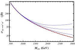
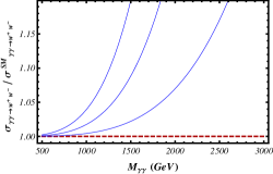
Figure 2: . Cross section (top) for $\gamma\gamma\to W_{L}^{+}W_{L}^{-}$ for unpolarized photons. The ratio of the ECLh and SM cross sections is provided in the lower plot. The red-dashed line correspond to the SM prediction and the solid blue ones our ECLh predictions for $a=c_{\gamma}=0$ and $(a_{1}-a_{2}+a_{3})=2\times 10^{-3},\,4\times 10^{-3},\,6\times 10^{-3}$, respectively from bottom to top in each plot.

3 $\gamma\gamma$–scattering in MCHM

In this section we show an explicit example of how our EFT description describes the small momentum regime of any underlying theory with the same symmetries and low-energy particle content.

In the context of the so called $SO(5)/SO(4)$ MCHM [8] it is assumed that some global symmetry breaking takes place at some scale $4\pi f>4\pi{\rm v}$ so that the group $G=SO(5)$ is spontaneously broken to the subgroup $H=SO(4)$. The corresponding NGBs live in the coset $G/H=S^{4}$. These four NGBs $\omega^{\alpha}$ are then identified with the Higgs-like boson $h$ and the three WBGBs needed for giving masses to the $W^{\pm}$ and $Z$ ($w^{\pm}=(\omega^{1}\mp i\omega^{2})/\sqrt{2}$, $z=\omega^{3}$, $h=\omega^{4}$).

The low-energy dynamics of the MCHM NGBs and the EW gauge bosons can be described through the gauged non-linear sigma model (NL$\sigma$M) [2, 8] (only operators with photons and NGBs are shown here),

$$\mathcal{L}^{\rm MCHM}_{2} = \frac{\displaystyle 1}{\displaystyle 2}D^{\mu}\Phi^{\,\,\dagger}\,D_{\mu}\Phi\,\mid_{S^{4}}$$

$$=\frac{1}{2}\,g_{\alpha\beta}(\omega)\,\partial^{\mu}\omega^{\alpha}\,\partial_{\mu}\omega^{\beta}$$

$$+\,i\,eA_{\mu}(\omega^{-}\partial^{\mu}\omega^{+}-\omega^{+}\partial^{\mu}\omega^{-})+e^{2}A^{2}\omega^{+}\omega^{-}.$$

with the $G$–fundamental representation vector $\Phi$ parametrizing the NGBs in the way

$$\Phi=\left(\begin{array}[]{c}\omega^{1}\\ \omega^{2}\\ \omega^{3}\\ c\omega^{4}+s\chi\\ -s\omega^{4}+c\chi\end{array}\right),\,\,\mbox{with }\chi=\left(f^{2}-\sum_{\alpha=1}^{4}(\omega^{\alpha})^{2}\right)^{1/2},$$ (22)

with $s=\sin\theta$, $c=\cos\theta$ and $\theta$ being the vacuum misalignment angle, with $\sin\theta={\rm v}/f$ [8]. The $S^{4}$ metric is given by

$$g_{\alpha\beta} = \delta_{\alpha\beta}+\frac{\omega^{\alpha}\omega^{\beta}}{f^{2}-\sum_{\alpha}(\omega^{\alpha})^{2}}\,.$$ (23)

Figure 3: MCHM one-loop diagrams for $\gamma\gamma\to w^{a}w^{b}$ at NLO.

The $\gamma\gamma$–scattering was considered in the framework of general $SO(N+1)/SO(N)$ gauged NL$\sigma$M [22] for low-energy QCD and the one-loop computation only involves the bubble and triangle diagrams (Fig. 3). The one-loop result at NLO is simply

$$A(\gamma\gamma\to zz)^{\rm NLO-loop}=A(\gamma\gamma\to hh)^{\rm NLO-loop}=\,-\,\frac{\displaystyle 1}{\displaystyle 4\pi^{2}f^{2}}\,,$$

$$A(\gamma\gamma\to w^{+}w^{-})^{\rm NLO-loop}=\,-\,\frac{\displaystyle 1}{\displaystyle 8\pi^{2}f^{2}}\,,$$

(24)

and $B^{\rm NLO-loop}=0$ in all cases. We find this in agreement with our ECLh result in Eqs. (14) and (15) by means of the relation $(1-a^{2})={\rm v}^{2}/f^{2}$ between $f$, ${\rm v}$ and the $hW^{+}W^{-}$ coupling $a$ in the $SO(5)/SO(4)$ MCHM [8].

We want to remark that the $\mathcal{L}_{2}^{\rm MCHM}$ is often written in exponential coordinates [8] rather than the $S_{4}$ parametrization used in this computation [2], leading to a low-energy Lagrangian with exactly the same structure as $\mathcal{L}_{2}$ in Eq. (6) but with precise predictions for the ECLh couplings. One can then use this Lagrangian in terms of exponential coordinates and compute the $\gamma\gamma$–scattering in the way done in this work (in that same parametrization), with all its complication and tricky diagrammatic cancelations. The final outcome agrees with (24), as expected. The lesson one draws is that, even though all the coset parametrizations yield the same outcome for a given on-shell amplitude, computations can be simpler for some choices of the NGB coordinates (we already saw this in our ECLh calculation in the previous section, where some vertices are absent in spherical coordinates and one has fewer diagrams to compute [2]). Likewise, in the exponential parametrization individual loop diagrams are suppressed with respect to the LO by ${\cal O}\left(p^{2}/(16\pi^{2}{\rm v}^{2})\right)$ and only after summing up all of them one finds that the full one-loop amplitude is actually suppressed by ${\cal O}\left(p^{2}/(16\pi^{2}f^{2})\right)$. On the other hand, in the $S_{4}$ coordinates each single diagram shown in Fig. 3 already carries the final suppression $p^{2}/(16\pi^{2}f^{2})$ with respect to the LO.

References

- [1] ATLAS Collaboration, Report No. ATLAS-CONF-2014-009; CMS Collaboration, Report No. CMS-PAS-HIG-14-009.
- [2] R.L. Delgado, A. Dobado, M.J. Herrero, J.J. Sanz-Cillero, JHEP 1407 (2014) 149 [arXiv:1404.2866 [hep-ph]].
- [3] S. Weinberg, Physica A96 (1979) 327.
- [4] J. Gasser and H. Leutwyler, Annals Phys. 158 (1984) 142; Nucl. Phys. B 250 (1985) 465; Nucl. Phys. B 250 (1985) 517.
- [5] M.B. Gavela, K. Kanshin, P.A.N. Machado and S. Saa, [arXiv:1409.1571 [hep-ph]].
- [6] G. Jikia, Nucl.Phys. B405 (1993) 24.
- [7] J. M. Cornwall, D. N. Levin and G. Tiktopoulos, Phys.Rev. D 10 (1974) 1145, Erratum-ibid. D 11 (1975) 972; C.E. Vayonakis, Lett.Nuovo Cim. 17 (1976) 383; B.W. Lee, C. Quigg and H.B. Thacker, Phys.Rev. D 16 (1977) 1519; G.J. Gounaris, R. Kogerler and H. Neufeld, Phys.Rev. D 34 (1986) 3257;
- [8] K. Agashe, R. Contino and A. Pomarol, Nucl. Phys. B 719, 165 (2005) [arXiv:hep-ph/0412089]; R. Contino, L. Da Rold and A. Pomarol, Phys. Rev. D 75, 055014 (2007) [arXiv:hep-ph/0612048]; R. Contino, D. Marzocca, D. Pappadopulo and R. Rattazzi, JHEP 1110 (2011) 081 [arXiv:1109.1570 [hep-ph]]; D. Barducci et al. JHEP 1309, 047 (2013) [arXiv:1302.2371 [hep-ph]].
- [9] T. Appelquist and C. W. Bernard, Phys. Rev. D 22 (1980) 200.
- [10] A. C. Longhitano, Phys. Rev. D 22 (1980) 1166; Nucl. Phys. B 188 (1981) 118.
- [11] R. Alonso, M.B. Gavela, L. Merlo, S. Rigolin and J. Yepes, Phys.Lett. B722 (2013) 330 [arXiv:1212.3305 [hep-ph]]; I. Brivio et al., JHEP 1403 (2014) 024 [arXiv:1311.1823 [hep-ph]].
- [12] A. Pich, I. Rosell and J.J. Sanz-Cillero, Phys.Rev.Lett. 110 (2013) 181801 [arXiv:1212.6769]; JHEP 1401 (2014) 157 [arXiv:1310.3121 [hep-ph]]
- [13] A. Manohar and H. Georgi, Nucl.Phys. B234 (1984) 189; J. Hirn and J. Stern, Phys.Rev. D73 (2006) 056001 [arXiv:hep-ph/0504277]; G. Buchalla and O. Cata, JHEP 1207 (2012) 101 [arXiv:1203.6510 [hep-ph]].
- [14] R. Urech, Nucl.Phys. B433 (1995) 234 [arXiv:hep-ph/9405341]
- [15] J. Bijnens and F. Cornet, Nucl. Phys. B 296 (1988) 557; J. F. Donoghue, B. R. Holstein and Y.C. Lin, Phys.Rev. D 37 (1988) 2423; J. Bijnens, S. Dawson and G. Valencia, Phys. Rev. D 44 (1991) 3555.
- [16] M. J. Herrero and E. Ruiz-Morales, Phys.Lett. B296 (1992) 397 [arXiv:hep-ph/9208220].
- [17] D. Espriu and B. Yencho, Phys. Rev D 87 (2013) 055017 [arXiv:1212.4158 [hep-ph]]; D. Espriu, F. Mescia and B. Yencho, Phys. Rev D 88 (2013) 055002 [arXiv:1307.2400 [hep-ph]]; D. Espriu and B. Mescia, Phys.Rev. D90 (2014) 015035 [arXiv:1403.7386 [hep-ph]]; R. L. Delgado, A. Dobado, F. J. Llanes-Estrada, J.Phys. G41 (2014) 025002 [arXiv:1308.1629 [hep-ph]]; JHEP 1402 (2014) 121 [arXiv:1311.5993 [hep-ph]].
- [18] Maria J. Herrero and Ester Ruiz Morales, Nucl.Phys. B418 (1994) 431-455 [arXiv:hep-ph/9308276].
- [19] S. Chatrchyan et al. (CMS Collaboration), JHEP 1307 (2013) 116 [arXiv:1305.5596 [hep-ex]].
- [20] M. Luszczak, A. Szczurek and C. Royon, [arXiv:1409.1803 [hep-ph]].
- [21] T. Han, Y.-P. Kuang and B. Zhang, Phys.Rev. D73 (2006) 055010 [arXiv:hep-ph/0512193].
- [22] A. Dobado and J. Morales, Phys.Lett. B 365 (1996) 264 [arXiv:hep-ph/9511244]; Phys.Rev. D 52 (1995) 2878