Stiffness effects on the dynamics of the bar-mode instability of Neutron Stars in full General Relativity

Abstract

We present results on the effect of the stiffness of the equation of state on the dynamical bar-mode instability in rapidly rotating polytropic models of neutron stars in full General Relativity. We determine the change in the threshold for the emergence of the instability for a range of the adiabatic $\Gamma$ index from 2.0 to 3.0, including two values chosen to mimic more realistic equations of state at high densities.

I Introduction

Non-axisymmetric deformations of rapidly rotating self-gravitating objects are a generic phenomenon in nature and are expected to appear in a wide range of astrophysical scenarios, like stellar core collapses Shibata and Sekiguchi (2005); Ott et al. (2005), accretion-induced collapses of white dwarfs Burrows et al. (2007), or mergers of two neutron stars Shibata et al. (2003a); Shibata et al. (2005). Over more than a decade, a considerable amount of work has been devoted to the search of unstable deformations that, even when starting from an axisymmetric configuration, can lead to a highly deformed, rapidly rotating, massive object Shibata et al. (2000); Baiotti et al. (2007); Kruger et al. (2010); Kastaun et al. (2010); Lai and Shapiro (1995); De Pietri et al. (2014). In the case of neutron stars, such deformations would lead to an intense emission of gravitational waves in the kHz range, potentially detectable on Earth within the next decade LIGO Scientific Collaboration et al. (2013) by next-generation gravitational-wave detectors such as Advanced LIGO Harry and LIGO Scientific Collaboration (2010), Advanced VIRGO, or KAGRA Somiya (2012).

Any insight on the possible astrophysical scenarios where such instabilities might be present would aid potential observations and their analysis and understanding. It is well-known that rotating neutron stars are subject to non-axisymmetric instabilities for non-radial axial modes with azimuthal dependence $\mathrm{e}^{im\phi}$ (with $m=1,2,\ldots$) when the instability parameter $\beta\equiv T/|W|$ (i.e. the ratio between the kinetic rotational energy $T$ and the gravitational potential energy $W$) exceeds a certain critical value $\beta_{c}$. This instability parameter plays an important role in the study of the so-called dynamical bar-mode instability, i.e. the $m=2$ instability which takes place when $\beta$ is larger than the threshold $\beta_{c}$  Baiotti et al. (2007). Previous results for the onset of the classical bar-mode instability have already shown that the critical value $\beta_{c}$ for the onset of the instability is not a universal quantity and it is strongly influenced by the rotational profile Shibata et al. (2003b); Karino and Eriguchi (2003), by relativistic effects Shibata et al. (2000); Baiotti et al. (2007), and, in a quantitative way, by the compactness Manca et al. (2007).

However, until the recent work in De Pietri et al. (2014), significant evidence of their presence when realistic EOSs are considered was missing. For example, in Corvino et al. (2010), using the unified SLy EOS Douchin and Haensel (2001), the presence of a shear-instability was shown, but there was no sign of the classical bar-mode instability and its critical behavior. The aim of the present work is to get more insight into the behavior of the classical bar-mode instability when the matter is described by EOSs with different stiffness. The investigations in the literature into its dependence on the stiffness of EOSs usually focused on values of $\Gamma$ (i.e. the adiabatic index of a polytropic EOS) in the range from $1$ to $2$ Lai and Shapiro (1995); Zink et al. (2007); Kastaun et al. (2010), while the expected value for a real neutron star is more likely higher, between $2$ and $3$, and probably around $\Gamma=2.75$ (at least in large portions of the interior). Such a choice for the EOS was already implemented in R. Oechslin et al. (2007), and also quite recently in Giacomazzo and Perna (2013); De Pietri et al. (2014). Its benefit is the ability to maintain the simplicity of a polytropic EOS and yet to obtain properties that resemble a more realistic case. Indeed, as it is shown in Fig. 1, a polytropic EOS with $K=30000$ and $\Gamma=2.75$ is qualitatively similar to the Shen proposal Shen et al. (1998a, b) in the density interval between $2\times 10^{13}\text{g/cm}^{3}$ and $10^{15}\text{g/cm}^{3}$, while a polytropic EOS with $K=80000$ and $\Gamma=3.00$ approximately resembles the SLy EOS for densities higher than $2\times 10^{14}\text{g/cm}^{3}$.

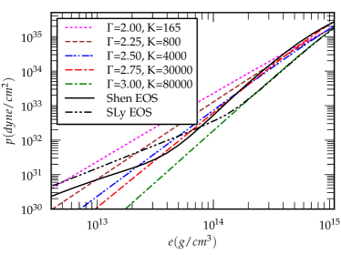
Figure 1: Diagram of the pressure $P$ vs. the energy density $e$ for all polytropic EOSs considered and two realistic EOSs for nuclear matter, namely (1) the Shen proposal Shen et al. (1998a, b); (2) the unified SLy prescription Douchin and Haensel (2001). The polytropic EOS with $\Gamma=2.75$ is close to the Shen EOS, while the case of $\Gamma=3.0$ is close to the SLy EOS, both above a certain density.

The organization of this paper is as follows. In Sec. II we describe the properties of the relativistic stellar models we investigated and briefly review the numerical setup used for their evolutions. In Sec. III we present and discuss our results, showing the features of the evolution and quantifying the effects of the compactness on the onset of the instability. Conclusions are given in Sec. IV. Throughout this paper we use a space-like signature $-,+,+,+$, with Greek indices running from 0 to 3, Latin indices from 1 to 3, and the standard convention for summation over repeated indices. Unless otherwise stated, all quantities are expressed in units in which $c=G=M_{\odot}=1$.

II Initial models and Numerical setup

We follow the same setup as in De Pietri et al. (2014) (only changing the EOS parameters $\Gamma$ and $K$), but for convenience the main ideas are summarized in the following section.

In this work we solve Einstein’s field equations

$$G_{\mu\nu}=8\pi T_{\mu\nu}\,,$$ (1)

where $G_{\mu\nu}$ is the Einstein tensor of the four-dimensional metric $g_{\mu\nu}$ and $T^{\mu\nu}$ is the stress-energy tensor of an ideal fluid. The energy-momentum tensor $T^{\mu\nu}$ can be parametrized as

$$T^{\mu\nu}=\rho\left(1+\epsilon+\frac{P}{\rho}\right)u^{\mu}u^{\nu}+Pg^{\mu\nu}\,,$$ (2)

where $\rho$ is the rest-mass density, $\epsilon$ is the specific internal energy of the matter, $P$ is the pressure, and $u^{\mu}$ is the matter $4$-velocity. The evolution equations for the matter follow from the conservation laws for the energy-momentum tensor $\nabla_{\mu}T^{\mu\nu}=0$ and the baryon number $\nabla_{\mu}(\rho u^{\mu})=0$, closed by an EOS of the type $P=P(\rho,\epsilon)$.

In order to generate the initial data, we use a $\Gamma$-type EOS of the form

$$P=K\rho^{\Gamma}\,,$$ (3)

where the following relation between $\epsilon$ and $\rho$ holds: $\epsilon=K\rho^{(\Gamma-1)}/(\Gamma-1)$. On the other hand, the evolution is performed using the so-called ideal-fluid ($\Gamma$-law) EOS

$$P=(\Gamma-1)\rho\epsilon\,,$$ (4)

that allows for increase of the internal energy by shock heating, if shocks are present.

We solve the above set of equations using the usual $3+1$ space-time decomposition, where the space-time is foliated as a tensor product of a three-space and a time coordinate $t$ (which is selected to be the $x^{0}$ coordinate). In this coordinate system the metric can be split as $g^{\mu\nu}=-n^{\mu}n^{\nu}+h^{\mu\nu}$, where $h^{\mu\nu}$ has only the spatial components different from zero and can be used to define a Riemannian metric $\gamma^{ij}=h^{ij}$ on each foliation. The vector $n^{\mu}$, that determines the direction normal to the 3-hypersurfaces of the foliation, is decomposed in terms of the lapse function $\alpha$ and the shift vector $\beta^{i}$, such that $n^{\mu}=\alpha^{-1}\cdot(1,\beta^{i})$. We also define the fluid three-velocity $v^{i}$ as the velocity measured by a local zero-angular momentum observer ($u^{i}=\alpha v^{i}-\beta^{i}$), while the Lorentz factor is $\alpha u^{0}=\sqrt{1-\gamma_{ij}v^{i}v^{j}}$. Within this formalism, the conservation of the baryon number suggests the use of the conserved variable $D=\sqrt{\gamma}\alpha u^{0}\rho$ with the property that $\int D\,d^{3}x=\text{const}$ along the time-evolution $t$.

II.1 Initial Data

The initial data of our simulations are calculated as stationary equilibrium solutions for axisymmetric and rapidly rotating relativistic stars in polar coordinates Stergioulas and Friedman (1995). We assume that the metric describing the axisymmetric and stationary relativistic star has the form

$$ds^{2}=-e^{\mu+\nu}dt^{2}+e^{\mu-\nu}r^{2} \sin^{2}\theta(d\phi-\omega dt^{2})^{2}$$

$$+e^{2\xi}(dr^{2}+r^{2}d\theta^{2})\,,$$ (5)

where $\mu$, $\nu$, $\omega$, and $\xi$ are space-dependent metric functions. Similarly, we assume the matter to be characterized by a non-uniform angular velocity distribution of the form

$$\Omega_{c}-\Omega=\frac{1}{\hat{A}^{2}r_{e}^{2}}\bigg{[}\frac{(\Omega-\omega)r^{2}\sin^{2}\theta e^{-2\nu}}{1-(\Omega-\omega)^{2}r^{2}\sin^{2}\theta e^{-2\nu}}\bigg{]}\,,$$ (6)

where $r_{e}$ is the equatorial stellar coordinate radius, $\Omega_{c}$ is the angular velocity at the center of the star, and the coefficient $\hat{A}$ is the measure of the degree of the differential rotation, which we set to be $\hat{A}=1$, analogous to works in the literature, and especially  De Pietri et al. (2014). Once imported onto the Cartesian grid, throughout the evolution we compute the coordinate angular velocity $\Omega$ on the $(x,y)$ plane as

$$\Omega=\frac{u^{\phi}}{u^{0}}=\frac{u^{y}\cos\phi-u^{x}\sin\phi}{u^{0}\sqrt{x^{2}+y^{2}}}\,.$$ (7)

Other characteristic quantities of the system such as the baryon mass $M_{0}$, the gravitational mass $M$, the internal energy $E_{\textrm{int}}$, the angular momentum $J$, the rotational kinetic energy $T$, the gravitational binding energy $W$ and the instability parameter $\beta$ are defined as Baiotti et al. (2007):

$$M_{0} \equiv\int d^{3}xD\,,$$ (8)

$$M \equiv\int d^{3}x(-2T^{0}_{0}+T^{\mu}_{\mu})\alpha\sqrt{\gamma}\,,$$ (9)

$$E_{\textrm{int}} \equiv\int d^{3}xD\varepsilon\,,$$ (10)

$$J \equiv\int d^{3}x\,T^{0}_{\phi}\alpha\sqrt{\gamma}\,,$$ (11)

$$T \equiv\int d^{3}x\Omega T^{0}_{\phi}\alpha\sqrt{\gamma}\,,$$ (12)

$$W \equiv T+E_{int}+M_{0}-M\,,$$ (13)

$$\beta \equiv T/|W|\,,$$ (14)

where $\alpha\sqrt{\gamma}$ is the square root of the four-dimensional metric determinant. Notice that the definitions of quantities such as $J$, $T$, $W$ and $\beta$ are meaningful only in the case of stationary axisymmetric configurations and should therefore be treated with care once the rotational symmetry is lost. All the equilibrium models considered here have been calculated using the relativistic polytropic EOS given in Eq. (3), and we have chosen the polytropic EOS parameters to be $\Gamma=[2.0$, $2.25$, $2.5$, $2.75$, and $3.0]$ for the adiabatic index, and $K=[165$, $800$, $4000$, $30000$, and $80000]$ for the polytropic constant respectively. This choice allows, for each pair of $\Gamma$ and $K$, a maximum neutron star mass of $\simeq 2.1M_{\odot}$. The exception is $\Gamma=2.75$, where simulation data from De Pietri et al. (2014), which allows for higher masses, were re-used to save computation time, given their identical numerical setup. Note that these values are different from the ones used in Manca et al. (2007) ($\Gamma=2.0,K=100$). Note, however, that the choice of $K$ does not change the results presented in this work. The actual value of the polytropic constant $K$ fixes the overall scale of the physical system; i.e. the assertion that we are generating and simulating a model with a given baryonic mass $M_{0}$ is related to the value chosen for $K$. Indeed, in order to claim that the threshold for the instability depends on the stiffness of the EOS, we need to eliminate the dependencies on the dimensional scales as well as on the chosen value of the polytropic constant $K$. An efficient way to do so is to extrapolate the result for $M_{0}\rightarrow 0$, which corresponds to the Newtonian limit, where the general relativistic effects can be neglected. Using the same procedure followed in Manca et al. (2007), we choose sequences of constant rest-mass density models among the following possible values for the total Baryon mass $M_{0}$ ($0.5$, $1.0$, $1.5$, $2.0$, and $2.5$ $M_{\odot}$). We restrict the values of the instability parameter $\beta$ to the range $[0.255,0.272]$, and we leave the analysis of models with lower values to future work. The initial conditions for the evolution have been generated using Nicholas Stergioulas’ RNS code Stergioulas and Friedman (1995). Any model can be uniquely determined by three parameters (once the value of the differential rotation parameter has been fixed to $\hat{A}=1$). We have decided to denote each of the generated models using the values of the adiabatic index $\Gamma$, the conserved baryonic mass $M_{0}$, and the $\beta$ parameter at $t=0$. As a consequence of this choice, in the rest of this paper we will refer to a particular model using the following notation. For example, G2.00M1.5b0.270 will denote a model with an adiabatic index of $2.0$, a conserved baryonic mass $M_{0}=1.5M_{\odot}$ and a value of the initial instability parameter $\beta=0.270$.

One of the main features of the generated models is that, due to the high rotation, none of them have the density maximum at the center of the star, but rather at some distance from it. This means that all of the models studied are characterized by a toroidal configuration, i.e. the maximum of the density is not on the rotational axis. As has been shown in De Pietri et al. (2014), there is not always a correlation between having a toroidal configuration and being unstable against the dynamical bar-mode instability.

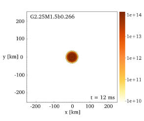
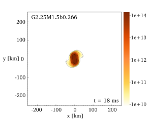
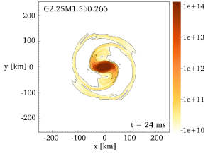
Figure 2: Snapshots of the rest-mass density $\rho$ in the $(x,y)$ plane for model G2.25M1.5b0.266 at different stages of the evolution, namely $t$ = 12 and 18 ms (top row), $t$ = 24 and 30 ms (bottom row). The color code is defined in terms of g/cm³. Additionally, isodensity contours are shown for $\rho=10^{10}$, $10^{11}$, $10^{12}$, $10^{13}$ and $10^{14}$ g/cm³.

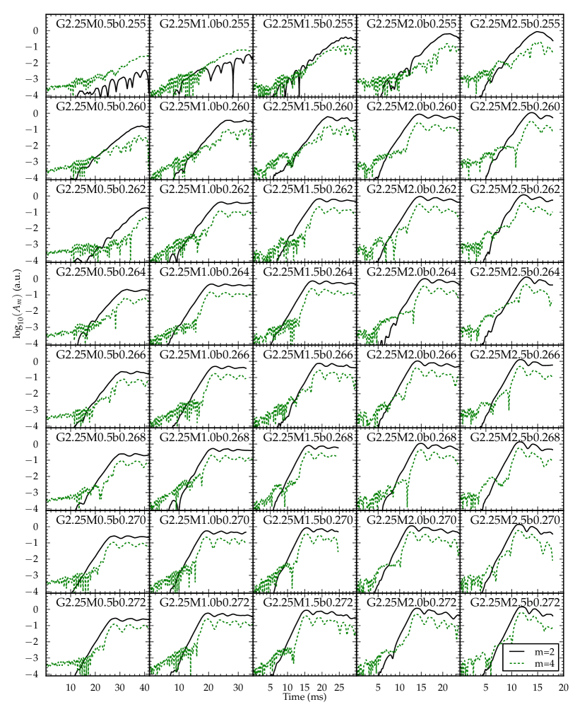
Figure 3: Mode dynamics for selected models that are characterized by a value of the instability parameter $\beta$ between 0.255 and 0.272. Almost all models with $\beta\geq 0.255$ show the typical dynamics one would expect for the dynamical $m=2$ bar mode instability. The exceptions are models G2.25M0.5b0.255 and G2.25M1.0b0.255, which are not well above $\beta_{c}$.

II.2 Numerical setup and evolution method

We use exactly the same numerical setup as in De Pietri et al. (2014). Because of this, we only briefly describe the specific methods used for this work together with the chosen, relevant, parameters. The reader is referred to Löffler et al. (2012) for a description of the Einstein Toolkit, and to De Pietri et al. (2014) for details about our particular setup.

The core of the code used for this work is the Einstein Toolkit Löffler et al. (2012); EinsteinToolkit , which is a free, publicly available, community-driven general relativistic (GR) code, capable of performing numerical relativity simulations that include realistic physical treatments of matter, electromagnetic fields Mösta et al. (2014), and gravity.

The Einstein Toolkit is built upon several open-source components that are widely used throughout the numerical relativity community. Only the ones which were actually used in this work are mentioned below. Many components of the Einstein Toolkit use the Cactus Computational Toolkit Cactus developers ; Goodale et al. (2003); Allen et al. (2011), a software framework for high-performance computing (HPC).

Within this study, the adaptive mesh refinement (AMR) methods implemented by Carpet Schnetter et al. (2004, 2006); Carpet have been used. Hydrodynamic evolution techniques are provided by the GRHydro package Baiotti et al. (2005); Hawke et al. (2005).

The evolution of the spacetime metric in the Einstein Toolkit is handled by the McLachlan package McLachlan . This code is auto-generated by Mathematica using Kranc Husa et al. (2006); Lechner et al. (2004); Kranc , implementing the Einstein equations via a $3+1-$dimensional split using the BSSN formalism Nakamura et al. (1987); Shibata and Nakamura (1995); Baumgarte and Shapiro (1999); Alcubierre et al. (2000, 2003).

Within this paper a fourth-order Runge-Kutta Runge (1895); Kutta (1901) method was used, and Kreiss-Oliger dissipation was applied to the curvature evolution quantities in order to damp high-frequency noise.

We use fourth-order finite difference stencils for the curvature evolution, $1+\log$ Alcubierre et al. (2003) slicing, and a $\Gamma$-driver shift condition Alcubierre et al. (2003). During time evolution, a Sommerfeld-type radiative boundary condition is applied to all components of the evolved BSSN variables as described in Alcubierre et al. (2000).

All presented results use the Marquina Riemann solver Donat and Marquina (1996); Aloy et al. (1999) and PPM (the piecewise parabolic reconstruction method) Colella and Woodward (1984). An artificial low-density atmosphere with $\rho_{\text{atm}}=10^{-10}$ is used, with a threshold of $\rho_{\text{atm\_reset}}=10^{-7}$ below which regions are set to be atmosphere. Hydrodynamical quantities are also set to be atmosphere at the outer boundary.

All evolutions presented use a mirror symmetry across the $(x,y)$ plane, consistent with the symmetry of the problem, which reduces the computational cost by a factor of $2$. Since we are not interested in investigating whether odd modes play any role, we present only results obtained by imposing an additional $\pi$-symmetry, reducing the computational cost by another factor of $2$.

III Results

As discussed in Sec. I and II, the goal of the present work is to study the matter instability that may develop in the case of rapidly differentially rotating relativistic star models, using different configurations of EOSs. The other important requirement we need to fulfill is that our study has to be computationally feasible. To achieve this goal, we need to evolve the largest number of models using the available amount of computational resources in the most efficient way. In selecting a numerical setting we can play with many parameters, namely: the location of the outer boundary, the number of refinement levels, the size and resolution of the finest grid and the symmetries to be imposed on the dynamics. All the simulations in the present work are performed using the same setting for the computational domain. More precisely, we use the same setup as in De Pietri et al. (2014): three box-in-box (covering the quarter space with $x\geq 0$ and $z\geq 0$) refinement levels, with boundaries at distances of $L=42,84,168$ from the origin of the coordinate system and grid spacings $dx,2\,dx,4\,dx$, respectively, where we set $dx=0.5$ (that correspond to a resolution $dx\simeq 0.738$ km). Using mirror symmetry across the $x-y$ plane and $\pi$ symmetry across the $y-z$ plane, this corresponds to a hierarchy of three computational grids, each one of size $85\times 169\times 85$ points plus ghost and buffer zones.

We have chosen to use this domain (conservative though large enough to capture the whole global dynamics of a bar-mode instability) in order to exclude any influence of the computational setup on observed differences between models. The actual size of the finest grid and the computational setup is determined by the most demanding models. Fig. 2 shows a few snapshots for the evolution of the rest-mass density $\rho$ at different times for a representative model, namely G2.25M1.5b0.266 which is characterized by $\Gamma=2.25$, $\beta=0.266$ and $M_{0}=1.5\,M_{\odot}$. This is indeed the typical evolution one would expect for a stellar model which is unstable against the dynamical bar-mode instability.

III.1 Analysis Methods

In order to compute the growth time of the instability, $\tau_{2}$, we use the quadrupole moments of the matter distribution $Q^{ij}$, computed in terms of the conserved density $D$ as

$$Q^{ij}=\int\!d^{3}\!x\;D\;x^{i}x^{j}\ .$$ (15)

In particular, we perform a nonlinear least-square fit of $Q^{xy}$ (the star spin axis is aligned in the $z$-direction), using the trial function

$$Q^{xy}(t)=Q^{xy}_{0}\mathrm{e}^{\frac{t}{\tau_{2}}}\cos(2\pi f_{2}t+\phi_{0})\,.$$ (16)

Using this trial function, we can extract the growth time $\tau_{2}$ and the frequency $f_{2}$ for the unstable $m=2$ modes. We also define the modulus $Q(t)$ as

$$Q\equiv\frac{1}{2}\sqrt{(2Q^{xy})^{2}+(Q^{xx}-Q^{yy})^{2}}\,,$$ (17)

and the distortion parameter $\eta(t)$ as

$$\eta\equiv\frac{2Q}{(Q^{xx}+Q^{yy})}\,.$$ (18)

Finally, we decompose the rest-mass density into its spatial rotating modes $P_{m}(t)$

$$P_{m}\equiv\int\mathrm{d}^{3}x\,\rho\mathrm{e}^{\mathrm{i}m\phi}$$ (19)

and the “amplitude” and “phase” of the $m$-th mode are defined as

$$A_{m}=|P_{m}|\,\quad\,\text{and}\,\quad\,\phi_{m}\equiv arg(P_{m})\,.$$ (20)

Despite their name, the amplitudes defined in Eq. (20) do not correspond to proper oscillation eigenmodes of the star but to global characteristics that are selected in terms of their spatial azimuthal shape. Eqs. (16)-(20) are expressed in terms of the coordinate time $t$, and therefore they are not gauge-invariant. However, the length scale of variation of the lapse function at any given time is always small when compared to the stellar radius, ensuring that events close in coordinate time are also close in proper time.

III.2 General features of the evolution above the threshold for the onset of the bar-mode instability

The general features of the evolution are common to all the models that show the expected dynamics in presence of the bar-mode $m=2$ instability. In Fig. 3 the “mode-dynamics” of most of the studied models with $\Gamma=2.25$ are shown as an example. For all these models (except for G2.25M0.5b0.255 and G2.25M1.0b0.255) it is indeed possible to extract the main features of the $m=2$ mode using the trial function detailed in Eq. (16). As in De Pietri et al. (2014), we decided to quantify the properties of the bar-mode instability by means of a non-linear fit, using the trial dependence of Eq. (16) on a time interval where the distortion parameter $\eta$ defined in Eq. (18) is between $1\%$ and $30\%$ of its maximum value.

The results of all these fits are collected in Tab. LABEL:tab:models in the Appendix, where we report for each model the maximum value assumed by the distortion parameter $\max(\eta)$, the time interval $[t_{i},t_{f}]$ selected for the fit, the value $\beta(t_{i})$ corresponding to the value of the instability parameter $\beta$ at the beginning of the fit interval and $\tau_{2}$ and $f_{2}$, the growth time and frequency that characterize the $m=2$ bar-mode instability, respectively.

III.3 Effects of the compactness on the threshold for the onset of the bar-mode instability

We have chosen to investigate the effect of the compactness on the classical bar-mode instability, following the same procedure as in Manca et al. (2007); De Pietri et al. (2014), but now for five stiffness values. We determined the critical value of the instability parameter $\beta$ for the onset of the instability by simulating, for each value of the stiffness, five sequences of initial models having the same value of $M_{0}$ but different values of $\beta$. For these simulations we decided to employ the same resolution $dx=0.5$ on the finest grid for all cases. This choice was motivated by the need to limit the computational cost.

We now restrict our analysis to the models for which we observed the maximum value of the distortion parameter $\eta$ to be greater than $0.20$ (see Tab. LABEL:tab:models). For these models, we explicitly checked that the reported unstable modes correspond to the classical bar-mode instability and not to a shear-instability by ensuring that the frequency of the mode divided by two is at most only marginally inside of the co-rotation band of the model.

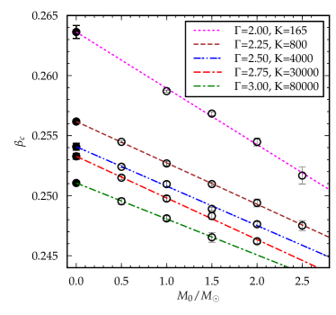
Figure 4: For each value of the adiabatic index $\Gamma$: the critical diagram relating the growth time $\tau_{2}$ of each unstable model to the value of the instability parameter $\beta$. Triangles represent the values corresponding to all the models listed in Tab. LABEL:tab:models. Specifically, we show the dependency of $\beta$ at the beginning of the time interval chosen for performing the fit of the $m=2$ mode growth (reported in Tab. LABEL:tab:models as $\beta(t_{i})$), on $\nicefrac{{1}}{{\tau_{2}^{2}}}$, in order to highlight the quality of the fit. For all the constant rest-mass sequences considered, we also report, with open circles, the extrapolated values $\beta_{c}$, which are used in the bottom right plot to show their dependency on the constant rest-mass, as well as the linear fit to the zero mass limit using Eq. (23).

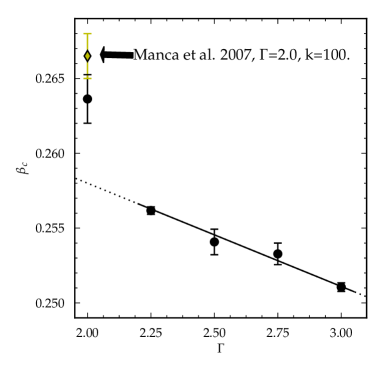
Figure 5: Dependency of the threshold $\beta_{c}^{N}$ of the bar-mode instability in the Newtonian limit of zero rest-mass on the stiffness of the EOS, i.e. on $\Gamma$, the exponent in the polytropic EOS. An approximate linear trend is visible in the range $2.25\lesssim\Gamma\lesssim 3.0$. The case of $\Gamma=2.0$ does not follow this trend, however, for reasons mentioned in Sec. III.3. Also mentioned is a result from a similar simulation Manca et al. (2007), confirming the high value of $\beta_{c}$ for $\Gamma=2.0$.

We have performed a fit for the growth time $\tau_{2}$ of the bar mode as a function of the instability parameter $\beta$ for twenty-one sequences of models with constant rest-mass ranging from 0.5 $M_{\odot}$ to 2.5 $M_{\odot}$, as shown in Fig. 4. We estimate the threshold for the onset of the instability using the extrapolation technique used in Manca et al. (2007); De Pietri et al. (2014) where we assume, in analogy with what expected in the Newtonian case, that the dependence of the frequency of the mode on $\beta$ is of the type

$$\sigma(\beta)=\Omega(\beta)\pm\sqrt{F(\beta)}\,,$$ (21)

where

$$F(\beta)=\frac{-1}{\left(\tau_{2}(\beta)\right)^{2}}\simeq A(\beta_{c}-\beta)\,.$$ (22)

$\Gamma$	M$[M_{\odot}]$	$\beta_{c}$			$A$
2.00	1.0		0.	25871(9)		11.3(1)
2.00	1.5		0.	2568(2)		19.0(3)
2.00	2.0		0.	2545(3)		27.8(8)
2.00	2.5		0.	2517(7)		36(2)
2.25	0.5		0.	25448(9)		19.4(2)
2.25	1.0		0.	2527(2)		35.6(5)
2.25	1.5		0.	2510(2)		54.0(7)
2.25	2.0		0.	2494(3)		76(2)
2.25	2.5		0.	2475(4)		96(2)
2.50	0.5		0.	2524(1)		39.6(3)
2.50	1.0		0.	2510(2)		67(1)
2.50	1.5		0.	2489(1)		94(1)
2.50	2.0		0.	2476(2)		123(2)
2.75	0.5		0.	2515(2)		46.0(7)
2.75	1.0		0.	2498(2)		71(1)
2.75	1.5		0.	2483(3)		94(2)
2.75	2.0		0.	2462(2)		111(1)
3.00	0.5		0.	2495(3)		92(2)
3.00	1.0		0.	2481(2)		136(2)
3.00	1.5		0.	2465(4)		179(5)

Table 1: Results for the fits of the critical value $\beta_{c}$ and the slope $A$ (see Eq. 22), with respect to the total baryon mass $M_{0}$, and for five seqences of various values of the adiabatic EOS index $\Gamma$.

$\Gamma$	$\beta_{c}^{N}$		$q$
2.00	0.	2636(5)	0.	0047(3)
2.25	0.	25617(8)	0.	00345(5)
2.50	0.	2541(3)	0.	0033(2)
2.75	0.	2533(2)	0.	0035(2)
3.00	0.	25106(9)	0.	00300(9)

Table 2: Results of the fits of the critical value $\beta_{c}^{N}$ ($\beta_{c}$ in the Newtonian limit of zero baryon mass), as well as $q$ (see Eq. 23) with respect to five different values of the adiabatic index $\Gamma$.

Results using different polytropic exponents $\Gamma$ cannot be directly compared to each other to infer the effects of considering a stiffer EOS. The issue is that when considering a polytropic EOS, one can change the units of measurement in such a way that the value of the polytropic constant $K$ is $1$. This means that by changing this value one effectively changes the mass scale and, in turn, the mass of the stellar model considered . Indeed, the assertion that for a star with mass $M_{0}=1.0M_{\odot}$ the threshold for the onset of the bar-mode instability is reduced to $0.2498(2)$ for $\Gamma=2.75$ from the higher value of $0.25871(9)$ for $\Gamma=2.0$ is susceptible to the choice of the mass scale determined by the choice of the values of the polytropic constants. The dependence on the choice of the mass scale can be eliminated by going to the zero-mass limit that corresponds to performing an extrapolation to the Newtonian limit of the results. This can be achieved by a linear fit of the reported values for the critical $\beta_{c}$ for the onset of the classical bar-mode instability in Tab. (1) as a function of the baryonic rest-mass (see Fig. 4). The result for this fit leads to the following expression for the critical $\beta_{c}$ as a function of the the total baryonic mass $M_{0}$:

$$\beta_{c}(M) =\beta_{c}^{N}-q\cdot M_{0}\,,$$ (23)

with different values of the constant depending on the adiabatic index $\Gamma$. These values are reported in Tab. 2 and shown on the bottom right box of Figure 4.

The extrapolated values for $\beta_{c}$ in the limit of zero baryonic mass for the relativistic stellar models then lead to a dependency on the compactness of the star alone, expressed as dependency on $\Gamma$, shown in Figure 5. As can be seen there, the dependency of $\beta_{c}$ on $\Gamma$ is, within errors, linear in the range $[2.25,3.0]$, while lower values of $\Gamma$ deviate notably. We also show results from Manca et al. (2007), using $\Gamma=2.0$ (and $K=100$), which show a similar deviation. The fact that the case of $\Gamma=2.0$ is special is not a surprise since in the Newtonian limit, i.e., for small values of central density the equilibrium configuration (see Chandrasekhar (1939)) of a non-rotational polytrope are described by the Lane-Emden equation, and the radius of the Star $R$ and its total mass $M$ are related to the central density $\rho_{c}$ as $R\propto\rho_{c}^{(\Gamma-2)/2}$ and $M\propto\rho_{c}^{(3\Gamma-4)/2}$. That means that the two values $\Gamma=4/3$ and $2$ are very special and represent the transition points to different behavior of the properties of the associated stellar models. In fact, for $\Gamma<\nicefrac{{4}}{{3}}$ we see that the mass decreases for increasing central density, and the models can not be stable, while $\Gamma=2$ marks a transition point in the relation between the radius of the star and the central density.

Our results show that the dependency of the threshold for the onset of the dynamical bar-mode instability on $\Gamma$ is not as large as the previously published results for $\Gamma=2.0$ Manca et al. (2007) and $\Gamma=2.75$ De Pietri et al. (2014) alone suggested, at least not close to the interesting value of $\Gamma=2.75$. Further investigation is necessary to clarify the exact dependency at values of $\Gamma$ lower than $2.25$.

IV Conclusions

We have presented a study of the dynamical bar-mode instability in differentially rotating NSs in full General Relativity for a wide and systematic range of values of the rotational parameter $\beta$ and the conserved baryonic mass $M_{0}$, using a polytropic/ideal-fluid EOS characterized by a range of values of the adiabatic index $\Gamma=[2.0,2.25,2.5,2.75$, and $3.0]$. In particular, we have evolved a large number of NS models belonging to twenty-one different sequences with a constant rest-mass ranging from $0.5$ to $2.5\,M_{\odot}$, with a fixed degree of differential rotation ($\hat{A}=1$), and with many different values of $\beta$ in the range $[0.255,0.278]$.

For all the models with a sufficiently high initial value of $\beta$ we observe the expected exponential growth of the $m=2$ mode which is characteristic of the development of the dynamical bar-mode instability. We compute the growth time $\tau_{2}$ for each of these bar-mode unstable models by performing a nonlinear least-square fit using a trial function for the quadrupole moment of the matter distribution. The growth time clearly depends on both the rest-mass and the rotation and in particular we find, in agreement with previous studies Manca et al. (2007); De Pietri et al. (2014), that the relation between the instability parameter $\beta$ and the inverse square of $\tau_{2}$, for each sequence of constant rest-mass, is linear.

This allows us to extrapolate the threshold value, $\beta_{c}$, for each sequence corresponding to the growth time going to infinity, using the same procedure already employed in Manca et al. (2007); De Pietri et al. (2014). Once the five values of $\beta_{c}$ for each value of $\Gamma$ have been computed, we are able to show that the dependency of $\beta_{c}$ on $\Gamma$ is, within errors, close to linear (see Fig. 5) in the the range $2.25\lesssim\Gamma\lesssim 3.0$. From this, we are able to perform a fit, predicting $\beta_{c}$ for a given value of $\Gamma$ between $2.25$ and $3$:

$$\beta_{c}\approx 0.2718-0.0069\cdot\Gamma\,.$$ (24)

However, we would like to stress that this should only be taken as rough estimate. In particular we do not claim an actual linear dependency of $\beta_{c}$ on $\Gamma$ in this range. Very likely the dependency is more complex. Further investigations are needed to clarify the full dependency of $\beta_{c}$ on $\Gamma$, especially for values of $\Gamma$ between $2.0$ and $2.25$.

Appendix A Model data

The results of all fits mentioned in Sec.III.2 are collected in the following Tab. LABEL:tab:models, where we report for each model the maximum value assumed by the distortion parameter $\max(\eta)$, the time interval $[t_{i},t_{f}]$ selected for the fit, the value $\beta(t_{i})$ corresponding to the value of the instability parameter $\beta$ at the beginning of the fit interval and $\tau_{2}$ and $f_{2}$, the growth time and frequency that characterize the $m=2$ bar-mode instability, respectively.

Table 3: Results for various quantities for all models, sorted by value of $\Gamma$, mass and $\beta$. We report for each model the maximum value assumed by the distortion parameter $\max(\eta)$, the time interval $[t_{i},t_{f}]$ selected for the fit, the value $\beta(t_{i})$ corresponding to the value of the instability parameter $\beta$ at the beginning of the fit interval and $\tau_{2}$ and $f_{2}$, the growth time and frequency that characterize the $m=2$ bar-mode instability, respectively.

model	$\max(\eta)$	$t_{i}$	$t_{f}$	$\beta(t_{i})$	$\tau_{2}$(ms)	$f_{2}$(kHz)
G2.00M1.0b0.255	0.012	-	-	-	-	-
G2.00M1.0b0.260	0.028	-	-	-	-	-
G2.00M1.0b0.262	0.107	-	-	-	-	-
G2.00M1.0b0.264	0.531	26.1	43.3	0.2633	4.388	0.251
G2.00M1.0b0.266	0.949	26.5	40.1	0.2653	3.680	0.248
G2.00M1.0b0.268	1.062	26.7	37.4	0.2673	3.200	0.246
G2.00M1.0b0.270	1.150	24.7	35.0	0.2694	2.879	0.244
G2.00M1.0b0.272	1.226	25.3	34.7	0.2714	2.656	0.241
G2.00M1.5b0.255	0.018	-	-	-	-	-
G2.00M1.5b0.260	0.692	22.5	40.2	0.2596	4.421	0.342
G2.00M1.5b0.262	0.860	21.7	32.4	0.2616	3.301	0.339
G2.00M1.5b0.264	0.982	24.2	34.1	0.2635	2.751	0.335
G2.00M1.5b0.266	1.086	21.5	29.2	0.2655	2.460	0.332
G2.00M1.5b0.268	1.171	19.1	26.9	0.2677	2.215	0.327
G2.00M1.5b0.270	1.243	20.4	27.1	0.2697	2.031	0.324
G2.00M1.5b0.272	1.315	19.1	25.7	0.2716	1.867	0.321
G2.00M2.0b0.255	0.167	-	-	-	-	-
G2.00M2.0b0.260	0.878	19.2	27.1	0.2596	2.614	0.436
G2.00M2.0b0.262	0.995	15.8	24.0	0.2617	2.239	0.430
G2.00M2.0b0.264	1.086	18.8	25.3	0.2637	1.933	0.427
G2.00M2.0b0.266	1.175	16.8	22.8	0.2658	1.804	0.421
G2.00M2.0b0.268	1.236	16.5	22.4	0.2677	1.637	0.413
G2.00M2.0b0.270	1.306	17.5	22.8	0.2696	1.533	0.407
G2.00M2.0b0.272	1.365	15.0	19.9	0.2718	1.443	0.402
G2.00M2.5b0.260	0.977	14.8	21.5	0.2598	1.829	0.539
G2.00M2.5b0.262	1.054	13.7	20.1	0.2617	1.702	0.537
G2.00M2.5b0.264	1.139	15.3	20.6	0.2637	1.488	0.523
G2.00M2.5b0.266	1.219	16.8	21.8	0.2655	1.354	0.519
G2.00M2.5b0.268	1.284	12.4	16.7	0.2677	1.290	0.510
G2.00M2.5b0.270	1.343	13.1	17.2	0.2697	1.257	0.500
G2.00M2.5b0.272	1.384	13.7	17.7	0.2717	1.173	0.493
G2.25M0.5b0.255	0.006	-	-	-	-	-
G2.25M0.5b0.260	0.492	19.6	31.5	0.2588	3.483	0.328
G2.25M0.5b0.262	0.571	24.5	34.8	0.2605	2.937	0.325
G2.25M0.5b0.264	0.650	19.1	27.7	0.2626	2.519	0.323
G2.25M0.5b0.266	0.717	18.9	26.5	0.2646	2.263	0.320
G2.25M0.5b0.268	0.786	19.4	26.3	0.2666	2.047	0.317
G2.25M0.5b0.270	0.851	16.8	23.3	0.2686	1.910	0.314
G2.25M0.5b0.272	0.909	17.9	24.0	0.2706	1.793	0.312
G2.25M1.0b0.255	0.131	-	-	-	-	-
G2.25M1.0b0.258	0.569	16.7	25.6	0.2571	2.585	0.470
G2.25M1.0b0.260	0.747	15.4	22.3	0.2591	2.085	0.466
G2.25M1.0b0.262	0.839	14.4	20.4	0.2610	1.827	0.462
G2.25M1.0b0.264	0.919	12.0	17.5	0.2632	1.611	0.458
G2.25M1.0b0.266	0.983	13.8	18.9	0.2651	1.500	0.453
G2.25M1.0b0.268	1.050	13.5	18.3	0.2671	1.410	0.450
G2.25M1.0b0.270	1.107	12.0	16.4	0.2693	1.303	0.444
G2.25M1.0b0.272	1.165	12.7	16.9	0.2712	1.230	0.438
G2.25M1.5b0.255	0.546	14.0	21.9	0.2539	2.542	0.612
G2.25M1.5b0.256	0.658	11.7	18.3	0.2552	2.092	0.611
G2.25M1.5b0.258	0.798	12.4	18.1	0.2572	1.740	0.601
G2.25M1.5b0.260	0.860	13.4	18.7	0.2590	1.491	0.597
G2.25M1.5b0.262	0.970	11.9	16.4	0.2612	1.362	0.590
G2.25M1.5b0.264	1.043	10.5	14.6	0.2632	1.215	0.585
G2.25M1.5b0.266	1.103	12.8	16.7	0.2650	1.141	0.578
G2.25M1.5b0.268	1.170	10.1	13.7	0.2673	1.068	0.573
G2.25M1.5b0.270	1.217	9.8	13.2	0.2691	1.003	0.564
G2.25M1.5b0.272	1.270	9.9	13.2	0.2712	0.963	0.557
G2.25M2.0b0.255	0.717	12.5	17.6	0.2539	1.681	0.764
G2.25M2.0b0.256	0.766	11.7	16.2	0.2549	1.536	0.754
G2.25M2.0b0.258	0.892	10.6	15.1	0.2572	1.335	0.747
G2.25M2.0b0.260	0.981	8.3	12.2	0.2593	1.137	0.736
G2.25M2.0b0.262	1.050	8.9	12.4	0.2612	1.035	0.731
G2.25M2.0b0.264	1.109	10.2	13.7	0.2630	0.984	0.718
G2.25M2.0b0.266	1.163	9.0	12.1	0.2651	0.916	0.711
G2.25M2.0b0.268	1.217	9.9	12.9	0.2668	0.875	0.702
G2.25M2.0b0.270	1.266	8.1	10.8	0.2692	0.809	0.691
G2.25M2.0b0.272	1.300	9.4	12.2	0.2706	0.797	0.679
G2.25M2.5b0.254	0.698	8.2	12.6	0.2529	1.493	0.925
G2.25M2.5b0.255	0.768	8.4	12.5	0.2537	1.260	0.927
G2.25M2.5b0.256	0.820	8.3	12.3	0.2548	1.223	0.918
G2.25M2.5b0.258	0.907	8.8	12.5	0.2568	1.086	0.910
G2.25M2.5b0.260	0.985	8.5	11.9	0.2587	0.960	0.898
G2.25M2.5b0.262	1.069	7.7	10.5	0.2608	0.864	0.878
G2.25M2.5b0.264	1.114	8.3	11.1	0.2625	0.818	0.873
G2.25M2.5b0.266	1.175	7.4	10.0	0.2649	0.765	0.861
G2.25M2.5b0.268	1.241	7.4	9.9	0.2673	0.734	0.842
G2.25M2.5b0.270	1.276	7.5	9.8	0.2690	0.695	0.830
G2.25M2.5b0.272	1.326	8.1	10.4	0.2708	0.666	0.814
G2.50M0.5b0.255	0.017	-	-	-	-	-
G2.50M0.5b0.258	0.188	-	-	-	-	-
G2.50M0.5b0.260	0.417	13.0	20.4	0.2578	2.171	0.475
G2.50M0.5b0.262	0.485	14.0	20.2	0.2596	1.852	0.471
G2.50M0.5b0.264	0.541	12.1	17.7	0.2620	1.621	0.467
G2.50M0.5b0.266	0.596	10.7	15.7	0.2642	1.465	0.465
G2.50M0.5b0.268	0.639	13.8	18.5	0.2656	1.382	0.460
G2.50M0.5b0.270	0.697	10.8	15.1	0.2683	1.259	0.456
G2.50M0.5b0.272	0.744	12.3	16.4	0.2698	1.207	0.451
G2.50M1.0b0.255	0.449	12.6	20.4	0.2530	2.288	0.656
G2.50M1.0b0.256	0.507	9.9	16.6	0.2545	1.942	0.654
G2.50M1.0b0.258	0.618	9.6	15.0	0.2571	1.575	0.650
G2.50M1.0b0.260	0.695	10.0	14.6	0.2585	1.389	0.644
G2.50M1.0b0.262	0.760	10.7	14.9	0.2603	1.251	0.637
G2.50M1.0b0.264	0.838	8.9	12.7	0.2626	1.116	0.632
G2.50M1.0b0.266	0.898	8.6	12.1	0.2652	1.029	0.627
G2.50M1.0b0.268	0.944	9.7	13.0	0.2665	0.975	0.621
G2.50M1.0b0.270	1.007	7.8	11.0	0.2687	0.912	0.615
G2.50M1.0b0.272	1.062	8.3	11.3	0.2705	0.868	0.608
G2.50M1.5b0.255	0.642	8.0	12.9	0.2536	1.513	0.829
G2.50M1.5b0.256	0.682	9.1	13.6	0.2544	1.380	0.817
G2.50M1.5b0.258	0.769	8.8	12.9	0.2569	1.160	0.812
G2.50M1.5b0.260	0.841	8.2	11.8	0.2584	1.060	0.806
G2.50M1.5b0.262	0.920	7.1	10.3	0.2607	0.940	0.796
G2.50M1.5b0.264	0.977	8.1	11.1	0.2625	0.890	0.790
G2.50M1.5b0.266	1.031	8.2	11.0	0.2645	0.824	0.781
G2.50M1.5b0.268	1.080	8.1	10.7	0.2669	0.767	0.770
G2.50M1.5b0.270	1.131	7.1	9.6	0.2685	0.739	0.763
G2.50M1.5b0.272	1.184	6.2	8.7	0.2705	0.708	0.754
G2.50M2.0b0.254	0.657	6.1	10.3	0.2530	1.239	1.011
G2.50M2.0b0.255	0.732	6.5	10.5	0.2538	1.154	1.001
G2.50M2.0b0.256	0.762	7.4	11.1	0.2544	1.080	0.998
G2.50M2.0b0.258	0.816	7.8	11.0	0.2559	0.968	0.985
G2.50M2.0b0.260	0.910	7.3	10.2	0.2585	0.864	0.977
G2.50M2.0b0.262	0.967	6.7	9.2	0.2599	0.796	0.967
G2.50M2.0b0.264	1.028	6.1	8.6	0.2630	0.733	0.953
G2.50M2.0b0.266	1.089	6.6	9.0	0.2641	0.698	0.941
G2.50M2.0b0.268	1.133	5.8	8.1	0.2664	0.652	0.929
G2.50M2.0b0.272	1.240	5.6	7.6	0.2708	0.595	0.901
G2.50M2.5b0.254	0.599	5.9	9.8	0.2521	1.191	1.215
G2.50M2.5b0.255	0.657	6.6	10.1	0.2529	1.106	1.214
G2.50M2.5b0.256	0.715	7.2	10.6	0.2535	0.951	1.209
G2.50M2.5b0.258	0.794	7.4	10.6	0.2555	0.938	1.197
G2.50M2.5b0.260	0.909	5.5	7.9	0.2584	0.750	1.176
G2.50M2.5b0.262	0.973	6.5	8.8	0.2599	0.714	1.159
G2.50M2.5b0.264	1.025	6.7	8.9	0.2615	0.668	1.137
G2.50M2.5b0.266	1.081	5.9	8.0	0.2641	0.622	1.124
G2.50M2.5b0.268	1.142	5.5	7.5	0.2663	0.577	1.104
G2.50M2.5b0.270	1.181	5.8	7.7	0.2681	0.559	1.087
G2.50M2.5b0.272	1.246	5.6	7.3	0.2703	0.522	1.060
G2.75M0.5b0.255	0.180	-	-	-	-	-
G2.75M0.5b0.258	0.341	14.3	22.4	0.2553	2.325	0.517
G2.75M0.5b0.260	0.415	10.7	16.9	0.2579	1.878	0.515
G2.75M0.5b0.262	0.473	12.0	17.4	0.2597	1.619	0.513
G2.75M0.5b0.264	0.524	10.8	15.7	0.2618	1.445	0.509
G2.75M0.5b0.266	0.578	9.2	13.7	0.2639	1.322	0.505
G2.75M0.5b0.268	0.616	11.8	16.1	0.2652	1.249	0.501
G2.75M0.5b0.270	0.666	9.9	13.8	0.2677	1.159	0.498
G2.75M0.5b0.272	0.707	9.9	13.7	0.2697	1.096	0.493
G2.75M1.0b0.255	0.480	10.4	17.0	0.2532	2.031	0.685
G2.75M1.0b0.258	0.618	9.9	15.0	0.2559	1.503	0.678
G2.75M1.0b0.260	0.709	7.6	11.9	0.2585	1.262	0.673
G2.75M1.0b0.262	0.790	6.6	10.4	0.2610	1.119	0.669
G2.75M1.0b0.264	0.830	8.6	12.2	0.2623	1.049	0.661
G2.75M1.0b0.266	0.888	8.8	12.0	0.2640	0.977	0.656
G2.75M1.0b0.268	0.945	7.0	10.0	0.2668	0.916	0.654
G2.75M1.0b0.270	0.996	7.2	10.2	0.2686	0.867	0.647
G2.75M1.0b0.272	1.042	8.4	11.2	0.2702	0.835	0.639
G2.75M1.0b0.274	1.097	6.7	9.3	0.2725	0.784	0.633
G2.75M1.0b0.276	1.131	7.4	9.9	0.2742	0.751	0.624
G2.75M1.5b0.255	0.664	7.7	12.3	0.2535	1.416	0.839
G2.75M1.5b0.260	0.867	6.9	10.3	0.2589	0.988	0.816
G2.75M1.5b0.262	0.926	7.4	10.5	0.2608	0.940	0.808
G2.75M1.5b0.264	0.989	6.8	9.7	0.2624	0.862	0.801
G2.75M1.5b0.266	1.034	7.1	9.8	0.2647	0.804	0.795
G2.75M1.5b0.268	1.082	7.0	9.6	0.2666	0.753	0.788
G2.75M1.5b0.270	1.151	6.7	9.2	0.2687	0.728	0.778
G2.75M1.5b0.272	1.163	7.2	9.5	0.2700	0.692	0.771
G2.75M1.5b0.274	1.241	7.2	9.4	0.2724	0.667	0.757
G2.75M1.5b0.276	1.269	6.8	8.9	0.2743	0.637	0.746
G2.75M2.0b0.250	0.411	6.9	12.6	0.2486	1.912	1.011
G2.75M2.0b0.255	0.748	6.6	10.3	0.2536	1.118	0.988
G2.75M2.0b0.258	0.876	5.7	8.8	0.2571	0.912	0.978
G2.75M2.0b0.260	0.923	6.7	9.6	0.2582	0.850	0.968
G2.75M2.0b0.262	0.999	6.4	9.2	0.2606	0.780	0.956
G2.75M2.0b0.264	1.059	5.9	8.3	0.2633	0.723	0.945
G2.75M2.0b0.266	1.118	5.2	7.5	0.2653	0.685	0.933
G2.75M2.0b0.268	1.160	5.9	8.1	0.2671	0.655	0.922
G2.75M2.0b0.270	1.192	5.2	7.3	0.2691	0.626	0.912
G2.75M2.0b0.272	1.249	5.5	7.5	0.2709	0.599	0.900
G2.75M2.0b0.274	1.294	5.3	7.2	0.2731	0.581	0.883
G3.00M0.5b0.255	0.139	-	-	-	-	-
G3.00M0.5b0.256	0.179	-	-	-	-	-
G3.00M0.5b0.258	0.255	7.1	12.0	0.2548	1.439	0.767
G3.00M0.5b0.260	0.293	7.4	11.4	0.2569	1.232	0.763
G3.00M0.5b0.262	0.345	6.0	9.5	0.2586	1.056	0.760
G3.00M0.5b0.264	0.367	7.7	11.1	0.2607	0.999	0.752
G3.00M0.5b0.266	0.415	6.2	9.2	0.2629	0.900	0.747
G3.00M0.5b0.268	0.442	8.0	10.8	0.2643	0.859	0.741
G3.00M0.5b0.270	0.478	6.9	9.6	0.2668	0.798	0.738
G3.00M0.5b0.272	0.514	5.6	8.1	0.2689	0.751	0.731
G3.00M1.0b0.254	0.312	4.9	9.5	0.2513	1.516	1.020
G3.00M1.0b0.255	0.363	6.1	10.4	0.2522	1.314	1.012
G3.00M1.0b0.256	0.363	9.3	13.4	0.2525	1.287	1.002
G3.00M1.0b0.258	0.462	6.2	9.8	0.2554	1.002	0.997
G3.00M1.0b0.260	0.535	6.2	9.1	0.2573	0.884	0.995
G3.00M1.0b0.262	0.590	6.2	8.9	0.2589	0.809	0.985
G3.00M1.0b0.264	0.641	5.8	8.4	0.2618	0.744	0.975
G3.00M1.0b0.266	0.686	6.0	8.3	0.2634	0.697	0.967
G3.00M1.0b0.268	0.738	4.7	6.8	0.2657	0.644	0.962
G3.00M1.0b0.270	0.781	6.3	8.4	0.2671	0.625	0.951
G3.00M1.0b0.272	0.829	5.2	7.2	0.2700	0.577	0.941
G3.00M1.5b0.254	0.418	4.8	8.4	0.2509	1.148	1.258
G3.00M1.5b0.256	0.498	7.3	10.4	0.2518	1.006	1.237
G3.00M1.5b0.258	0.574	5.6	8.5	0.2544	0.820	1.236
G3.00M1.5b0.260	0.651	4.7	7.1	0.2573	0.733	1.228
G3.00M1.5b0.262	0.723	5.3	7.6	0.2592	0.660	1.211
G3.00M1.5b0.264	0.755	5.2	7.3	0.2605	0.619	1.195
G3.00M1.5b0.266	0.830	3.2	5.1	0.2641	0.570	1.188
G3.00M1.5b0.270	0.917	5.1	6.8	0.2669	0.514	1.156
G3.00M1.5b0.272	0.967	5.1	6.8	0.2693	0.497	1.141

References

- Shibata and Sekiguchi (2005) M. Shibata and Y.-i. Sekiguchi, Phys. Rev. D 71, 024014 (2005), eprint arXiv:astro-ph/0412243.
- Ott et al. (2005) C. D. Ott, S. Ou, J. E. Tohline, and A. Burrows, Astrophys.J. 625, L119 (2005), eprint astro-ph/0503187.
- Burrows et al. (2007) A. Burrows, L. Dessart, E. Livne, C. D. Ott, and J. Murphy, Astrophys. J. 664, 416 (2007), eprint arXiv:astro-ph/0702539.
- Shibata et al. (2003a) M. Shibata, K. Taniguchi, and K. Uryu, Phys. Rev. D 68, 084020 (2003a), eprint arXiv:gr-qc/0310030.
- Shibata et al. (2005) M. Shibata, K. Taniguchi, and K. Uryu, Phys. Rev. D 71, 084021 (2005), eprint arXiv:gr-qc/0503119.
- Shibata et al. (2000) M. Shibata, T. W. Baumgarte, and S. L. Shapiro, Astrophys.J. 542, 453 (2000), eprint astro-ph/0005378.
- Baiotti et al. (2007) L. Baiotti, R. De Pietri, G. M. Manca, and L. Rezzolla, Phys. Rev. D 75, 044023 (2007), eprint arXiv:astro-ph/0609473.
- Kruger et al. (2010) C. Kruger, E. Gaertig, and K. D. Kokkotas, Phys.Rev. D81, 084019 (2010), eprint 0911.2764.
- Kastaun et al. (2010) W. Kastaun, B. Willburger, and K. D. Kokkotas, Phys.Rev. D82, 104036 (2010), eprint 1006.3885.
- Lai and Shapiro (1995) D. Lai and S. L. Shapiro, Astrophys.J. 442, 259 (1995), eprint astro-ph/9408053.
- De Pietri et al. (2014) R. De Pietri, A. Feo, L. Franci, and F. Löffler, Phys. Rev. D 90, 024034 (2014), eprint arXiv:gr-qc/1403.8066.
- LIGO Scientific Collaboration et al. (2013) LIGO Scientific Collaboration, Virgo Collaboration, J. Aasi, J. Abadie, B. P. Abbott, R. Abbott, T. D. Abbott, M. Abernathy, T. Accadia, F. Acernese, et al., ArXiv e-prints (2013), eprint 1304.0670.
- Harry and LIGO Scientific Collaboration (2010) G. M. Harry and LIGO Scientific Collaboration, Classical and Quantum Gravity 27, 084006 (2010).
- Somiya (2012) K. Somiya, Classical and Quantum Gravity 29, 124007 (2012), eprint 1111.7185.
- Shibata et al. (2003b) M. Shibata, S. Karino, and Y. Eriguchi, Mon.Not.Roy.Astron.Soc. 343, 619 (2003b), eprint astro-ph/0304298.
- Karino and Eriguchi (2003) S. Karino and Y. Eriguchi, Astrophys. J. 592, 1119 (2003).
- Manca et al. (2007) G. M. Manca, L. Baiotti, R. De Pietri, and L. Rezzolla, Class. Quantum Grav. 24, S171 (2007), eprint arXiv:0705.1826 [astro-ph].
- Corvino et al. (2010) G. Corvino, L. Rezzolla, S. Bernuzzi, R. De Pietri, and B. Giacomazzo, Classical Quantum Gravity 27, 114104 (2010), eprint 1001.5281.
- Douchin and Haensel (2001) F. Douchin and P. Haensel, Astron. Astrophys. 380, 151 (2001), eprint arXiv:astro-ph/0111092.
- Zink et al. (2007) B. Zink, N. Stergioulas, I. Hawke, C. D. Ott, E. Schnetter, and E. Müller, Phys. Rev. D 76, 024019 (2007), eprint astro-ph/0611601.
- R. Oechslin et al. (2007) R. Oechslin, H.-T. Janka, and A. Marek, A&A 467, 395 (2007), URL http://dx.doi.org/10.1051/0004-6361:20066682.
- Giacomazzo and Perna (2013) B. Giacomazzo and R. Perna, Astrophys.J. 771, L26 (2013), eprint 1306.1608.
- Shen et al. (1998a) H. Shen, H. Toki, K. Oyamatsu, and K. Sumiyoshi, Nucl. Phys. A 637, 435 (1998a), URL http://user.numazu-ct.ac.jp/~sumi/eos.
- Shen et al. (1998b) H. Shen, H. Toki, K. Oyamatsu, and K. Sumiyoshi, Prog. Th. Phys. 100, 1013 (1998b).
- Douchin and Haensel (2001) F. Douchin and P. Haensel, Astron. Astrophys. 380, 151 (2001), eprint arXiv:astro-ph/0111092.
- Stergioulas and Friedman (1995) N. Stergioulas and J. L. Friedman, Astrophys. J. 444, 306 (1995).
- Löffler et al. (2012) F. Löffler, J. Faber, E. Bentivegna, T. Bode, P. Diener, R. Haas, I. Hinder, B. C. Mundim, C. D. Ott, E. Schnetter, et al., Class. Quantum Grav. 29, 115001 (2012), eprint arXiv:1111.3344 [gr-qc].
- (28) EinsteinToolkit, Einstein Toolkit: Open software for relativistic astrophysics, URL http://einsteintoolkit.org/.
- Mösta et al. (2014) P. Mösta, B. C. Mundim, J. A. Faber, R. Haas, S. C. Noble, T. Bode, F. Löffler, C. D. Ott, C. Reisswig, and E. Schnetter, Classical and Quantum Gravity 31, 015005 (2014), eprint arXiv:1304.5544 [gr-qc].
- (30) Cactus developers, Cactus Computational Toolkit, URL http://www.cactuscode.org/.
- Goodale et al. (2003) T. Goodale, G. Allen, G. Lanfermann, J. Massó, T. Radke, E. Seidel, and J. Shalf, in Vector and Parallel Processing – VECPAR’2002, 5th International Conference, Lecture Notes in Computer Science (Springer, Berlin, 2003), URL http://edoc.mpg.de/3341.
- Allen et al. (2011) G. Allen, T. Goodale, G. Lanfermann, T. Radke, D. Rideout, and J. Thornburg, Cactus Users’ Guide (2011), URL http://www.cactuscode.org/Guides/Stable/UsersGuide/UsersGuideStable.pdf.
- Schnetter et al. (2004) E. Schnetter, S. H. Hawley, and I. Hawke, Class. Quantum Grav. 21, 1465 (2004), eprint arXiv:gr-qc/0310042.
- Schnetter et al. (2006) E. Schnetter, P. Diener, E. N. Dorband, and M. Tiglio, Class. Quantum Grav. 23, S553 (2006), eprint arXiv:gr-qc/0602104.
- (35) Carpet, Carpet: Adaptive Mesh Refinement for the Cactus Framework, URL http://www.carpetcode.org/.
- Baiotti et al. (2005) L. Baiotti, I. Hawke, P. J. Montero, F. Löffler, L. Rezzolla, N. Stergioulas, J. A. Font, and E. Seidel, Phys. Rev. D 71, 024035 (2005), eprint arXiv:gr-qc/0403029.
- Hawke et al. (2005) I. Hawke, F. Löffler, and A. Nerozzi, Phys. Rev. D 71, 104006 (2005), eprint arXiv:gr-qc/0501054.
- (38) McLachlan, McLachlan, a public BSSN code, URL http://www.cct.lsu.edu/~eschnett/McLachlan/.
- Husa et al. (2006) S. Husa, I. Hinder, and C. Lechner, Comput. Phys. Commun. 174, 983 (2006), eprint arXiv:gr-qc/0404023.
- Lechner et al. (2004) C. Lechner, D. Alic, and S. Husa, Analele Universitatii de Vest din Timisoara, Seria Matematica-Informatica 42 (2004), ISSN 1224-970X, eprint arXiv:cs/0411063.
- (41) Kranc, Kranc: Kranc assembles numerical code, URL http://kranccode.org/.
- Nakamura et al. (1987) T. Nakamura, K. Oohara, and Y. Kojima, Prog. Theor. Phys. Suppl. 90, 1 (1987).
- Shibata and Nakamura (1995) M. Shibata and T. Nakamura, Phys. Rev. D 52, 5428 (1995).
- Baumgarte and Shapiro (1999) T. W. Baumgarte and S. L. Shapiro, Phys. Rev. D 59, 024007 (1999), eprint arXiv:gr-qc/9810065.
- Alcubierre et al. (2000) M. Alcubierre, B. Brügmann, T. Dramlitsch, J. A. Font, P. Papadopoulos, E. Seidel, N. Stergioulas, and R. Takahashi, Phys. Rev. D 62, 044034 (2000), eprint arXiv:gr-qc/0003071.
- Alcubierre et al. (2003) M. Alcubierre, B. Brügmann, P. Diener, M. Koppitz, D. Pollney, E. Seidel, and R. Takahashi, Phys. Rev. D 67, 084023 (2003), eprint arXiv:gr-qc/0206072.
- Runge (1895) C. Runge, Mathematische Annalen 46, 167 (1895), ISSN 0025-5831, URL http://dx.doi.org/10.1007/BF01446807.
- Kutta (1901) W. Kutta, Z. Math. Phys. 46, 435 (1901).
- Donat and Marquina (1996) R. Donat and A. Marquina, J. Comp. Phys. 125, 42 (1996).
- Aloy et al. (1999) M. Aloy, J. Ibanez, J. Marti, and E. Muller, Astrophys. J. Suppl. 122, 151 (1999), eprint arXiv:astro-ph/9903352.
- Colella and Woodward (1984) P. Colella and P. R. Woodward, J. Comp. Phys. 54, 174 (1984).
- Chandrasekhar (1939) S. Chandrasekhar, An introduction to the study of stellar structure (Dover Publications, New Haven, USA, 1939), revised edition 1958.