Phase-resolved spectroscopy of low frequency quasi-periodic oscillations in GRS 1915+105

Abstract

X-ray radiation from black hole binary (BHB) systems regularly displays quasi-periodic oscillations (QPOs). In principle, a number of suggested physical mechanisms can reproduce their power spectral properties, thus more powerful diagnostics which preserve phase are required to discern between different models. In this paper, we first find for two Rossi X-ray Timing Explorer (RXTE) observations of the BHB GRS 1915+105 that the QPO has a well defined average waveform. That is, the phase difference and amplitude ratios between the first two harmonics vary tightly around a well defined mean. This enables us to reconstruct QPO waveforms in each energy channel, in order to constrain QPO phase-resolved spectra. We fit these phase resolved spectra across 16 phases with a model including Comptonisation and reflection (Gaussian and smeared edge components) to find strong spectral pivoting and a modulation in the iron line equivalent width. The latter indicates the observed reflection fraction is changing throughout the QPO cycle. This points to a geometric QPO origin, although we note that the data presented here do not entirely rule out an alternative interpretation of variable disc ionisation state. We also see tentative hints of modulations in the iron line centroid and width which, although not statistically significant, could result from a non-azimuthally symmetric QPO mechanism.

1 Introduction

Low frequency quasi-periodic oscillations (hereafter QPOs), are regularly observed in the X-ray light curves of accreting compact objects in binary systems (e.g.van der Klis 2006). Their properties are tightly correlated with the observed spectral transitions in both black hole and neutron star binaries (BHBs and NSBs). In BHBs, the QPO fundamental frequency evolves from $\sim 0.1-30$ Hz as the spectrum transitions from the power law dominated hard state to the multicoloured disc blackbody dominated soft state (e.g. Wijnands & van der Klis 1999). The multicoloured blackbody is well understood as a geometrically thin, optically thick accretion disc (Shakura & Sunyaev 1973; Novikov & Thorne 1973) and the power law as Compton up-scattering of cool disc photons by energetic electrons in some optically thin (optical depth $\tau\sim 1$) cloud near the black hole (Thorne & Price 1975; Sunyaev & Truemper 1979). This cloud is often interpreted as the evaporated inner accretion disc (the inner flow; Esin et al. 1997; Done et al. 2007; Gilfanov 2010), or alternatively the base of a jet (Markoff et al. 2005; Fabian et al. 2012). The QPO signal originates in the most part from this Comptonising cloud (Sobolewska & Życki 2006; Axelsson et al. 2013). When Comptonised photons illuminate the disc, some fraction are scattered into the line of sight with a characteristic reflection spectrum including a prominent iron K_α line.

Suggested QPO mechanisms include relativistic precession models (Stella & Vietri 1998; Wagoner et al. 2001; Schnittman et al. 2006; Ingram & Done 2012a) and disc instability models (e.g. Tagger & Pellat 1999; Cabanac et al. 2010). All of these models can, in principle, reproduce the power spectral properties of QPOs. Determining the QPO phase dependence of the spectrum provides a powerful diagnostic tool to discern between different models. This is relatively simple for periodic oscillations such as eclipses and NS pulsations. In this case, phase-resolved spectra can be constrained by folding the light curve (e.g. Gierliński et al. 2002; Wilkinson et al. 2011). However, simply folding the light curve is not appropriate for QPOs, since their phase does not evolve linearly, or even deterministically with time (e.g. Morgan et al. 1997). In fact, it is important to ask the question: what makes QPOs quasi-periodic rather than purely periodic? Specifically, does the oscillation have an underlying waveform, whereby the phase differences between different harmonics and harmonic amplitude ratios are not random but instead have a well defined average? We cannot tell using just the power spectrum and the cross spectrum between energy bands if an oscillation with two strong harmonics has some average underlying waveform or if it is simply uncorrelated ‘noise’ with a set of harmonically related characteristic frequencies.

Here, in section 2 we show for two Rossi X-ray Timing Explorer (RXTE) observations of the BHB GRS 1915+105 that the amplitude ratio and phase difference between the first two QPO harmonics do indeed vary tightly around mean values (as is suggested by measurements of the bicoherence of the signal: Maccarone et al. 2011). This indicates that there is some average underlying waveform which, in sections 3 and 4, we estimate for each energy channel in order to constrain QPO phase-resolved spectra. Then, in section 5, we fit these spectra with a model consisting of Comptonisation and reflection to find strong spectral pivoting and a modulation in the iron line equivalent width.

2 The phase difference between QPO harmonics

Before we can phase-resolve the QPO, we must determine if there even exists a well defined average underlying waveform. If the stochastic process producing the QPO is instead uncorrelated between harmonic frequencies, the meaning of phase resolved spectra is difficult to asses. In this section, we show that there is indeed some average QPO waveform by measuring the harmonic amplitudes and the phase difference between harmonics.

2.1 What makes QPOs quasi-periodic?

We can consider this question in general by representing the count rate in the $k^{\rm th}$ time bin, $x_{k}$, as

$$x_{k}=\mu+\sum_{j=1}^{N/2}|X_{j}|\cos[2\pi jk/N-\varphi_{j}],$$ (1)

where $X_{j}=|X_{j}|e^{i\varphi_{j}}$ is the discrete Fourier transform (DFT) of $x_{k}$, $\mu$ is the mean count rate and there are $N$ time bins in the light curve. Hereafter, we refer to $\varphi_{j}$ as the phase offset of the $j^{\rm th}$ Fourier frequency (which has a frequency $\nu_{j}=j/[N~{}dt]$).

Splitting a long light curve which contains a QPO into many short segments of length $N$ time bins allows us to study how the DFT at the QPO harmonic frequencies varies between segments. Specifically, we can measure how the amplitude and phase offsets vary with time for each harmonic. If the oscillation was instead perfectly periodic, the amplitude and phase offset of each harmonic would remain constant. Since a QPO is only quasi-periodic, these conditions must not all be met. Thus, perhaps a more insightful question is: how does the amplitude and phase offset vary for each QPO harmonic? Previous work has already shown that the amplitude of the first two QPO harmonics in XTE J1550-564 correlate with the flux over a $\sim 3$ s timescale (Heil et al. 2011; also see Ingram & Done 2011). We note that due to this, the Timmer & Koenig (1995) algorithm for generating maximally stochastic time series is not appropriate for simulating realistic QPO signals. In contrast, little is thus far known about how the phase offsets vary.

Here, we consider variations in the phase offsets of the first two QPO harmonics. Defining the phase offset of the $j^{\rm th}$ QPO harmonic as $\Phi_{j}$ (as opposed to the phase offset of the $j^{\rm th}$ Fourier frequency, $\varphi_{j}$), we can write

$$\Phi_{2}=2(\Phi_{1}+\psi),$$ (2)

where $\psi$ is the phase difference between the harmonics, defined on the interval $0$ to $\pi$. From this definition, $\psi$ is the radians of the first harmonic by which the $2^{\rm nd}$ harmonic lags the $1^{\rm st}$. In general, $\psi$ will vary with time (i.e. from segment to segment), but does it vary around a well defined mean value or simply at random? In this paper, we study two observations of GRS 1915+105 which are described in the following subsection.

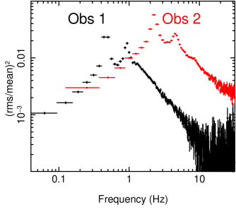
Figure 1: White noise subtracted power spectra, plotted in units of frequency $\times$ power, for observations 1 (black) and 2 (red). Both display strong QPOs with at least two harmonics.

2.2 Data

We consider two RXTE observations of GRS 1915+105 with observational IDs 60701-01-28-00 (hereafter observation 1) and 20402-01-15-00 (hereafter observation 2), both in the $\chi$ variability class as defined by Belloni et al. (2000). The white noise subtracted power spectra of the full band light curves of both observations are shown in Figure 1. Both clearly show QPOs with strong contributions from the first two harmonics, which we fit with Lorentzian functions in order to measure the centroid $\nu_{0}$ and half width at half maximum (HWHM) for each component. For the fundamental we measure $\nu_{0}=0.46$ Hz and HWHM$=0.0275$ Hz for observation 1 and $\nu_{0}=2.26$ Hz and HWHM$=0.14$ Hz for observation 2. These two observations have been selected since they both have a high count rate, a strong QPO and a (comparatively) long exposure. Observation 1 was taken on March 6^th 2002 and observation 2 was taken on February 9^th 1997. The time averaged spectra for these observations can be well modelled by an absorbed Comptonisation model with a soft power law ($\Gamma\sim 2.3$ and $\Gamma\sim 2$ for observations 1 and 2 respectively), in addition to a strong contribution from a broad iron $K_{\alpha}$ emission line. Neither spectra require a direct disc component, but this is simply due to the large absorption column around GRS 1915+105, plus the hard response of the PCA. Whereas observation 2 was observed to be radio faint (Muno et al. 2001), there are no radio data taken simultaneous with observation 1 (Prat et al. 2010). However, Yan et al. (2013) define two branches for GRS 1915+105 on a plot of hardness ratio ($7-60$ keV flux / $2-7$ keV flux) against QPO frequency and find that branch 1 and 2 approximately correspond respectively to radio loud and quiet intervals (Figure 1 therein). Since observation 1 falls in branch 1, it is likely the source was radio loud at this time.

We selected times when 3 and 5 Proportional Counter Units (PCUs) were on for observations 1 and 2 respectively, in addition to applying standard RXTE good time selections (elevation greater than $10$ degrees and offset less than $0.02$ degrees) using ftools from the heasoft 6.15 package. After this screening, observations 1 and 2 contain 9.680 ks and 10.272 ks of good time respectively, and we measure mean count rates of 1744 c/s/PCU and 816 c/s/PCU. We extract light curves using saextrct. Both observations were taken in the ‘binned’ mode “B_8ms_16A_0-35_H”, which has a timing resolution of $dt=1/128$ s and provides 16 energy channels sensitive to the energy range $\sim 2-15$ keV. For the purposes of spectral fitting, we generate response matrices using pcarsp and background spectra using runpcabackest. We also apply $0.5\%$ systematic errors using grppha to account for uncertainties in the response of the PCA and ignore the poorly calibrated lowest energy channel.

2.3 Measuring the harmonic amplitudes and phase differences

We split both light curves into $M$ segments, with each segment containing $N$ time bins of duration $dt=1/128$ s. We may expect the QPO to stay roughly coherent (i.e. periodic to a good approximation) for $Q$ cycles, where $Q=\nu_{0}/{\rm FWHM}$ is the quality factor (${\rm FWHM}=2~{}{\rm HWHM}$). We therefore choose $N$ to ensure that each segment contains $\sim Q$ cycles of the fundamental, whilst also requiring $N$ to be an integer power of two in order to use the Fast Fourier Transform algorithm. Thus $N\sim 1/({\rm FWHM}~{}dt)$, giving $N=2048$, $M=605$ for observation 1 and $N=512$, $M=2548$ for observation 2.

We first investigate the relative strength of each harmonic. We measure the average rms in each harmonic using our multi-Lorentzian fit to the power spectrum: the integral from zero to infinity of a Lorentzian component gives the squared rms in that component. This gives $\langle\sigma_{1}\rangle=(9.6\pm 0.2)\%$, $\langle\sigma_{2}\rangle=(6.7\pm 0.2)\%$ for observation 1 and $\langle\sigma_{1}\rangle=(12.7\pm 0.1)\%$, $\langle\sigma_{2}\rangle=(7.6\pm 0.1)\%$ for observation 2. We now wish to measure $\sigma_{1}$ and $\sigma_{2}$ for each segment. Since the power spectrum calculated for only one segment is very noisy, we cannot reliably fit a multi-Lorentzian model for each segment. Instead, we use the centroids and widths from our existing fit and calculate the power in the range $\nu=\nu_{0}\pm{\rm HWHM}$ for each segment. We then calculate the normalisation of a Lorentzian function which has this integral in this narrow range (i.e. similar to a bolometric correction). In Figure 2, we plot a histogram of the harmonic ratio calculated for each segment, $\sigma_{1}/\sigma_{2}$, normalised by the number of segments in each observation. We see that, consistent with previous work (Heil et al. 2011), the harmonic ratio appears to vary around a well defined mean, although the distribution is more narrowly peaked for observation 1.

If the phase difference between the harmonics, $\psi$, also has some preferred value, we can conclude that the QPO does indeed have a well defined mean waveform. For each segment, we calculate $\psi$ from the phase offsets of the $1^{\rm st}$ and $2^{\rm nd}$ QPO harmonics, $\Phi_{1}$ and $\Phi_{2}$ respectively, using the formula

$$\psi=[\Phi_{2}/2-\Phi_{1}]_{\rm mod\pi},$$ (3)

where the ‘${\rm mod\pi}$’ signifies that each $\psi$ value is defined on the interval from $0$ to $\pi$. The phase offset for the $j^{\rm th}$ Fourier frequency, which is simply the argument of the DFT $X_{j}$, is given by

$$\tan\varphi_{j}=\frac{\Im[X_{j}]}{\Re[X_{j}]}.$$ (4)

We define $\Phi_{j}=\varphi_{jq}$, where $\nu_{q}$ is the nearest Fourier frequency to the centroid of the fundamental. Since the width of each Fourier frequency bin is $d\nu=1/(N~{}dt)$, this means that $d\nu\sim{\rm FWHM}$. Thus, by defining the QPO phase offsets in this way, we are effectively averaging across the width of the fundamental.

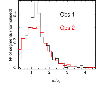
Figure 2: Histogram of measured harmonic ratios for observations 1 (black) and 2 (red).

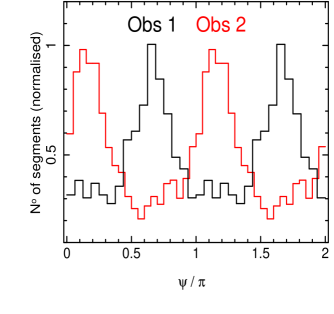
Figure 3: Histogram of measured values of the phase difference between harmonics, $\psi$, for observations 1 (black) and 2 (red). The distributions each show two peaks purely because $\psi$ is defined on the interval $0\rightarrow\pi$ and we have shown two intervals by repeating the pattern.

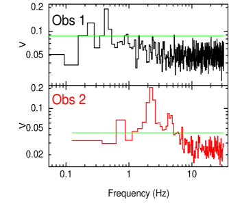
Figure 4: We measure the phase difference between the Fourier component at each frequency, $\nu_{j}$, and twice that frequency, $2\nu_{j}$, for many segments. $V$ is Kuiper’s statistic, which assess the likelihood that the phase differences are compatible with being drawn from a random distribution. Values of $V$ above the green line are not compatible with a random distribution ($>99.7\%$ confidence). Both observations show a very strong peak at the fundamental QPO frequency, and the higher signal-to-noise observation 2 also shows significant peaks at higher harmonics (see text for details).

Figure 3 shows a histogram of the $\psi$ values measured for each segment. Here, we have defined phase bins on the interval $0\leq\psi<\pi$ but we plot values up to $2\pi$ by repeating the pattern. We see that for both observations, the phase difference $\psi$ is clearly distributed around a mean value, indicating that $\Phi_{1}$ and $\Phi_{2}$ do indeed correlate. Note that the distribution only has one true peak: the second peak results because we have repeated the pattern to account for the cyclical nature of $\psi$. We formally confirm that the data are incompatible with a random distribution using Kuiper’s statistic (see e.g. Press et al. 1992). This is similar to a KS-test, only adapted to also be appropriate for a cyclical quantity such as the one we are considering. It involves calculating the cumulative distribution function of the data and measuring its maximum distance above, $D_{+}$, and below, $D_{-}$, a theoretical cumulative distribution function. The probability that the data belongs to the theoretical distribution can be calculated from Kuiper’s statistic, $V=D_{+}+D_{-}$, and the number of data points in the observed distribution. As expected, this confirms the distributions shown in Figure 3 are not random with a significance $>>5\sigma$.

To compare the QPO with the broad band noise, we calculate Kuiper’s statistic for the series of phase differences between each Fourier component ($\nu_{j}$) and the component with twice its frequency ($2\nu_{j}$). In Figure 4 we plot $V$ against $\nu_{j}$ for all $1\leq j<N/4$ (since $2\nu_{N/4}$ is the Nyquist frequency). The green lines indicate $3\sigma$ confidence intervals: if $V$ is above the green line for a frequency $\nu_{j}$, the phase difference between the components at $\nu_{j}$ and $2\nu_{j}$ are not randomly distributed (at least with confidence $>99.7\%$). For both observations, all pairs of broadband noise frequencies are consistent with a random phase difference, in sharp contrast to the phase difference between $1^{\rm st}$ and $2^{\rm nd}$ QPO harmonics. We also see evidence of an interaction between a sub-harmonic and the fundamental. Observation 2 additionally shows a deviation from random phase differences between the $2^{\rm nd}$ and $4^{\rm th}$ and even the $3^{\rm rd}$ and $6^{\rm th}$ harmonics. This may provide a sensitive method for detecting previously undetectable QPO harmonics. In this paper, however, we concentrate on the interaction between $1^{\rm st}$ and $2^{\rm nd}$ harmonics, which contain the bulk of the variability power.

To measure the mean phase difference between $1^{\rm st}$ and $2^{\rm nd}$ QPO harmonics, $\langle\psi\rangle$, we must account for the cyclical nature of $\psi$. For a particular trial value of $\langle\psi\rangle$, the distance between $\psi_{m}$ and $\langle\psi\rangle$ (in the $m^{\rm th}$ segment) is

$$d_{m}=\begin{cases}\delta&\text{if $\delta<\pi/2$,}\\ \pi-\delta&\text{otherwise,}\end{cases}$$ (5)

where $\delta=|\psi_{m}-\langle\psi\rangle|$. This can be understood by picturing all the $\psi_{m}$ values on a circle (with only $\pi$ radians around its circumference): there are always two paths around the circle to any point; $d_{m}$ is the shortest of these two paths. We find the $\langle\psi\rangle$ value which minimises $\chi^{2}=\sum_{m=1}^{M}d_{m}^{2}$ using Brent’s method (e.g. Press et al. 1992), and calculate the standard deviation on the mean as $\chi_{\rm min}/M$. This gives $\langle\psi\rangle/\pi=0.667\pm 9.9\times 10^{-3}$ and $\langle\psi\rangle/\pi=0.133\pm 4.6\times 10^{-3}$ for observations 1 and 2 respectively. The fact that the phase difference is different between observations indicates that the underlying QPO waveform has changed. In future, we will study how $\langle\psi\rangle$ depends on QPO frequency for many observations.

3 Reconstruction of the QPO waveform

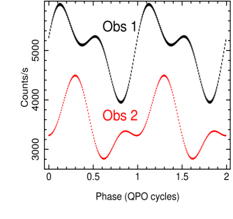
Figure 5: Reconstructed QPO waveform for both observations. The shape of the waveform differs dramatically between observations 1 (black) and 2 (red).

Since we are able to measure average values for the amplitudes of, and phase difference between, the first two QPO harmonics, we can reconstruct an average underlying waveform. That is, we can define a periodic function of QPO phase, $\phi$, given by

$$w(\phi)=\mu\left[1+\sqrt{2}\sum_{j=1}^{J}\langle\sigma_{j}\rangle\cos(j\phi-\Phi_{j})\right],$$ (6)

where $\langle\sigma_{j}\rangle$ is the measured fractional rms in the $j^{\rm th}$ harmonic and $\Phi_{j}$ is the phase offset of the $j^{\rm th}$ harmonic. Here, the phase offset of the first harmonic is arbitrary: we are interested in the shape of the waveform rather than the starting point. We set $\Phi_{1}=\pi/2$. The phase difference between each harmonic and the first, in contrast, is important. Here we only consider $J=2$ harmonics since these contain the bulk of the power.

It is simple to measure the mean count rate $\mu$, and we use our measurement of the phase difference between the first two harmonics, $\langle\psi\rangle$, from the previous section. We also use our measurements of $\langle\sigma_{1}\rangle$ and $\langle\sigma_{2}\rangle$ from the previous section. We then use equation 6 to obtain an estimate of the average underlying QPO waveform. How exactly this relates to the physical QPO mechanism depends, in general, on the details of the processes generating the waveform and those de-cohering it (Ingram & van der Klis 2013). If the decohering process is highly non-linear, this may introduce a bias in our estimate of the true underlying waveform, or indeed may make such a true waveform difficult to define. In the absence of a full understanding of all the processes de-cohering the QPO, we define our waveform as a periodic function with the average QPO properties.

To obtain an error estimate, we use our measurements of $\sigma_{j}$ and $\psi$ for each segment (see the previous section), along with a measurement of the mean count rate for each segment, in order to calculate a waveform (using equation 6) for each segment. This gives $M$ functions $w_{m}(\phi)$, in addition to our estimate for the average waveform, $w(\phi)$. For each discrete value of $\phi$ considered, we calculate the standard deviation on the mean of the $w_{m}(\phi)$ points around the average $w(\phi)$. Figure 5 shows the resulting waveforms for both observations, evaluated for 128 QPO phases. Our reconstructed waveforms have small errors since we can measure each of the five parameters in equation 6 accurately, and there are correlations between these parameters. Note that different phase values in Figure 5 are not statistically independent of one another, and so we do not expect to see a scatter in the data consistent with the size of the error bars, nor will we be able to reduce the size of the errors by binning on phase. The errors determined here are errors on the function $w(\phi)$ and the phase values are instances rather than intervals.

We note that this is not the first derivation of a QPO waveform. Tomsick & Kaaret (2001) used a folding method to estimate the QPO waveform in observations of GRS 1915+105. This method, as expected, yields similar results to ours but crucially, it implicitly assumes that the phase difference between QPO harmonics is constant, which we find to only be approximately true.

4 Phase resolving method

Now that we can reconstruct a waveform for the full band, we can reconstruct a waveform for each energy channel by generalising equation 6 to

$$w(E,\phi)=\mu(E)\left\{1+\sqrt{2}\sum_{j=1}^{J}\langle\sigma_{j}(E)\rangle\cos[j\phi-\Phi_{j}(E)]\right\}.$$ (7)

For each energy channel, we extract a light curve for which it is again simple to measure the mean. We fit a multi-Lorentzian model to the power spectrum of each light curve and define the rms in the $1^{\rm st}$ and $2^{\rm nd}$ QPO harmonics as the integral of the corresponding Lorentzian function (following e.g. Axelsson et al. 2014). Figure 6 shows the measured fractional rms in the $1^{\rm st}$ (circles) and $2^{\rm nd}$ (points) harmonics as a function of channel energy.

The most obvious way of measuring the phase offsets would perhaps be to measure $\langle\psi\rangle$ for each energy channel using the method described in section 2.3. We would then need to measure the phase difference between energy bands of the first harmonic. Instead, we maximise signal to noise by measuring the phase lag at each harmonic, $\Delta_{j}(E)$, between each energy band, $E$, and the full band. With our measure of $\langle\psi\rangle$ for the full band, we can calculate the phase offsets using the formulae

$$\Phi_{1}(E) = \pi/2+\Delta_{1}(E)$$

$$\Phi_{2}(E) = 2(\Phi_{1}(E)+\langle\psi\rangle)+\Delta_{2}(E).$$ (8)

We calculate the lags in the usual way by taking the cross spectrum between each subject band, $s(E,t)$, and the reference band $r(t)$ (e.g. van der Klis et al. 1987), which we define as the full band with the subject band subtracted to avoid correlating $s(E,t)$ with itself (Uttley et al. 2014). For each harmonic, we evaluate the complex cross spectrum, $C_{j}(E)$, at the nearest Fourier frequency to the centroid frequency of that harmonic. The phase lag is then

$$\tan\Delta_{j}(E)=\frac{\Im C_{j}(E)}{\Re C_{j}(E)}.$$ (9)

Figure 7 shows the lags as a function of energy for the $1^{\rm st}$ (circles) and $2^{\rm nd}$ (points) harmonics.

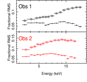
Figure 6: Fractional rms for the $1^{\rm st}$ (circled points) and $2^{\rm nd}$ (no marker) QPO harmonics as a function of energy for both observations.

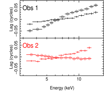
Figure 7: Phase lags between a given energy channel and the full band for the $1^{\rm st}$ (circled points) and $2^{\rm nd}$ (no marker) QPO harmonics.

We now have all the information required to reconstruct a waveform for each energy channel using equation 7. Note from equations 8 that, even though we have only measured the phase difference between harmonics, $\langle\psi\rangle$, in the full band, the waveforms in different channels are free to have different shapes. This is because their phase offsets depend on the phase lags between energy bands which in general can be different for different harmonics. Light curves for three channels (with the energy at the centre of the channel labeled) are shown in Figure 8. We see that the waveform shape changes with energy channel for both observations considered here. We note that, much like the case of the full band considered in the previous section, the relation between the waveform measured for each energy channel and the physical QPO mechanism can potentially be biased by highly non-linear decohering effects. If the nature of these effects is strongly energy dependent, this could bias the energy dependence of the measured waveforms. Again, in the absence of a full understanding of the de-cohering mechanism, we define the waveform in each energy channel as a periodic function with the average QPO properties.

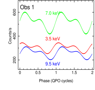
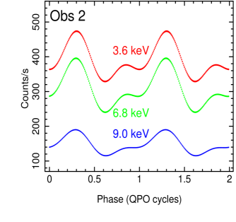
Figure 8: Waveforms reconstructed using Equation 7 for three different energy channels. The energy at the centre of the channel is labeled.

We calculate an error estimate for the waveform in each channel in the same way as we did for the full band: we calculate a waveform for each segment and measure the dispersion around $w(E,\phi)$. This involves the additional step of calculating the phase lags $\Delta_{j}(E)$ for each segment. We can now plot the count rate as a function of energy for any given number of QPO phases: i.e. we can plot and analyse QPO phase resolved spectra. In Figure 9, we plot spectra for 4 QPO phases, represented as a ratio to the phase averaged spectrum. For both observations, we see strong spectral pivoting. Even though different values of QPO phase are not statistically independent, it is important to note that different energy channels are statistically independent. This means that we can use $\chi^{2}$ statistics in order to fit models to the spectrum for each phase and study how spectral parameters vary with QPO phase. We note that Miller & Homan (2005) studied the phase resolved behaviour of ‘Type-C’ QPOs in GRS 1915+105 (in fact, they studied our observation 2) by selecting spectra from high and low flux intervals. Our technique takes this further, allowing us to study the evolution of spectral parameters with QPO phase rather than for just two phases. Phase resolved spectroscopy has also been used to investigate the ‘Heartbeat’ state of GRS 1915+105 (Neilsen et al. 2011) and also the QPO in the Active Galactic Nucleus RE J1034+396 (Maitra & Miller 2010), although we note that all previous analyses have assumed the phase difference between harmonics to be constant, in contrast to this Paper.

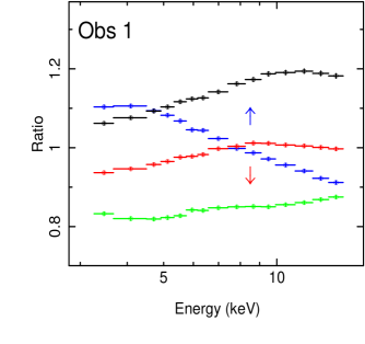
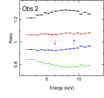
Figure 9: The spectrum corresponding to 4 QPO phases, plotted as a ratio to the mean spectrum. Phases are selected to be representative of rising (blue), peak (black), falling (red) and trough (green) intervals. For observation 1, these phases are $\phi=$ 0, 0.1875, 0.625 and 0.75 QPO cycles respectively. For observation 2, they are $\phi=$ 0, 0.3125, 0.4375 and 0.625 cycles. For both observations, we clearly see spectral pivoting.

5 Spectral Modelling

We use xspec version 12.8 to fit the spectral model

$$\textsc{phabs}~{}*~{}\textsc{smedge}~{}*~{}(\textsc{ewgaus}~{}*~{}\textsc{nthComp}),$$ (10)

for 16 QPO phases. Here, phabs accounts for interstellar absorption for a given hydrogen column density $N_{h}$ and a given set of elemental abundances. We fix $N_{h}$ to a reasonable value consistent with previous analyses of these observations (e.g. Miller & Homan 2005) and assume the solar abundances of Wilms et al. (2000). The model nthComp (Zdziarski et al. 1996; Życki et al. 1999) calculates a Comptonisation spectrum consisting of a power law (photon index $\Gamma$) between low and high energy breaks, governed respectively by the seed photon and electron temperature, $kT_{bb}$ and $kT_{e}$. Since the data do not extend beyond $15$ keV, we cannot constrain the electron temperature so arbitrarily fix $kT_{e}=100$ keV. In contrast, we allow $\Gamma$ and $kT_{bb}$ to go free in the fit. The model smedge mimics the shape of a smeared reflection edge in the PCA bandpass and has input parameters $E_{\rm Edge}$, $f$ and $W$, which govern the position, depth and width of the reflection edge. In our fits, we fix these parameters to reasonable values. We find that the data do not statistically require a disc component due to the high column density surrounding GRS 1915+105 and the hard response of the PCA.

Since the equivalent width (EW) of the iron line is of interest, we define a new xspec model ewgaus, which is simply a Gaussian function with three parameters: centroid energy in keV ($E_{c}$) width in keV ($\sigma$) and EW in eV. Thus, the only difference to the standard xspec Gaussian function is that the EW is an input parameter rather than the line flux. We define this as a convolution model, since we must determine from the continuum the normalisation required to give the line the specified EW, for which we use Brent’s method. Note that, even though this is defined as a convolution model, this is not the mathematical operation: we simply add the Gaussian to the continuum, we define a convolution model purely to allow the continuum to be input to the model.

In the following subsection we present the results of our spectral fits for both observations. We allow 5 parameters of physical interest to be free in the fit as a function of QPO phase: the continuum parameters $\Gamma$ and $kT_{bb}$, plus the iron line parameters $E_{c}$, $\sigma$ and EW. For each of these parameters, we use an f-test comparing a fit with the parameter held constant to the best fit model to asses if it varies with QPO phase, and with what statistical significance.

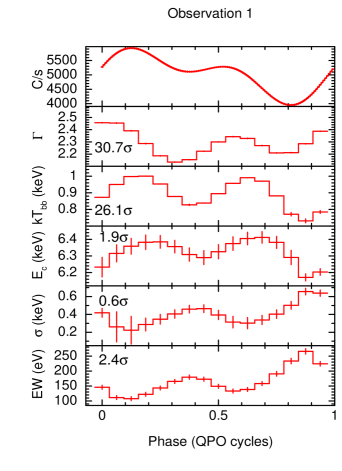
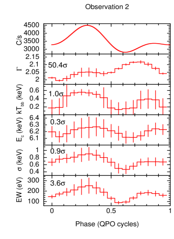
Figure 10: Best fit parameters of our spectral fit plotted as a function of QPO phase. Both observations show highly significant spectral pivoting and we see a modulation in the relative strength of the iron line. The statistical significance of each modulation is quoted in the corresponding plot.

5.1 Results

5.1.1 Observation 1

We achieve a good fit with $\chi^{2}_{\nu}=158.07/144$ by freezing the hydrogen column density to $N_{\rm h}=5.2\times 10^{22}~{}{\rm cm}^{-2}$ and the smedge parameters to $E_{\rm Edge}=8.25$ keV, $f=0.3$ and $W=5$ keV. Figure 10 (left) shows the evolution of the 5 physically interesting parameters across 16 phases, with the full band waveform also reproduced at the top for reference (error bars are all $1\sigma$). We quote with what statistical significance each spectral parameter varies with QPO phase in the top-left corner of each panel. We see that $\Gamma$ and $kT_{bb}$ vary with a very high significance and both contain a strong $2^{\rm nd}$ harmonic. We also see that the iron line parameters vary, also with a strong $2^{\rm nd}$ harmonic, but non above the 3$\sigma$ level. Clearly, the points as plotted are incompatible with a constant but, when each iron line parameter is held constant for an alternative fit, changes in other parameters can, to some extent compensate. Note that the systematic nature of these modulations does not alone indicate they are real. A random $1\sigma$ fluctuation in, say, the measured rms can potentially result in a systematic looking modulation in the phase resolved spectrum. We must therefore use the f-tests to asses significance.

5.1.2 Observation 2

We again achieve a good fit with $\chi^{2}_{\nu}=144.06/144$, this time by freezing the hydrogen column density to $N_{\rm h}=5.4\times 10^{22}~{}{\rm cm}^{-2}$ and the smedge parameters to $E_{\rm Edge}=8.5$ keV, $f=0.3$ and $W=5$ keV. We plot the QPO phase evolution of the best fit parameters on the right of Figure 10. We again see a highly significant modulation of $\Gamma$ but this time $kT_{bb}$ only varies with $1\sigma$ confidence. The modulations in the iron line centroid and width are not statistically significant, but the EW varies with $3.6\sigma$ confidence. Our results are consistent with those of Miller & Homan (2005), who analysed spectra for this observation selected for high and low flux intervals.

5.2 Interpretation

We can conclude with high statistical confidence that the spectral index varies with QPO phase for both observations and also that the parameter $kT_{bb}$ varies with phase in observation 1. We also find a $>3\sigma$ modulation in the iron line EW for observation 2. Here, we discuss possible interpretations of these modulations as well as speculating about what modulations we may expect to see in the iron line shape for higher quality data sets.

5.2.1 Continuum parameters

We can picture the observed spectral variability, on the simplest level, as a power law with changing index and normalisation. If the total flux in a broad energy band lags the power law index, hard photons will lag soft photons. This is because $\Gamma$ is a proxy for spectral softness, and thus this means the peak flux lags the softest spectrum, or in other words the hardest spectrum lags the peak flux. This corresponds to a positive gradient in the lag vs energy spectrum. For observation 1, we do indeed find that the total PCA count rate lags $\Gamma$ by $\approx 0.29$ cycles for the fundamental and $\approx 0.06$ cycles for the $2^{\rm nd}$ harmonic, which is consistent with the positive gradient seen in Figure 7 for the lag spectrum of both harmonics. For observation 2, we instead find that the total count rate leads $\Gamma$ by $\approx 0.42$ cycles for the fundamental and lags $\Gamma$ by $\approx 0.12$ cycles, which is consistent with the negative gradient of the lag spectrum of the fundamental and the positive gradient for the $2^{\rm nd}$ harmonic. It is this spectral pivoting which is at the heart of the generic models for alternating phase lags recently proposed by Misra & Mandal (2013) and Shaposhnikov (2012).

Physically, this spectral pivoting can either be attributed to changes in Comptonisation or perhaps changes in the reflection hump, which we do not model here. If the pivoting were exclusively down to a changing flux in the reflection hump, the spectral hardness would track the reflection fraction. We would therefore expect an anti-correlation between $\Gamma$ and the iron line EW - i.e. a phase difference of 0.5 cycles for each harmonic. Since the phase difference for the strong $2^{\rm nd}$ harmonic is $\sim 0.24$ and $\sim 0.23$ cycles for observation 1 and 2 respectively, it seems likely that there is at least some pivoting of the Comptonised spectrum itself. This can result from modulations in the temperature, $kT_{e}$, and/or optical depth, $\tau$, of the corona. The simple formula $\Gamma-1\propto 1/[\tau kT_{\rm e}]$ approximates the case of thermal Compton scattering (Pietrini & Krolik 1995). Although we cannot discern between these two interpretations here, we note that it should be possible to measure both the electron temperature and the shape of the reflection hump as a function of QPO phase by carrying out a similar analysis with the Nuclear Spectroscopic Telescope ARray (NuStar; Harrison 2013), which has a high spectral resolution and reasonable throughput up to $\sim 70$ keV.

The fits for observation 1 also clearly require $kT_{bb}$ to change with QPO phase with very high significance. Since we do not detect a direct disc component, it is difficult to interpret exactly what this means. This could really be a measure of the seed photon temperature. Alternatively, the nthComp component could be mimicking a combination of weak direct disc emission plus Comptonised emission. If the true disc flux were to increase in this scenario, the low energy cut-off of the nthComp component would move to a lower energy in order to find a fit. Thus a minimum in $kT_{bb}$ could, counter-intuitively, correspond to a maximum in direct disc flux. We are unable to determine if this is the case with these data, but will investigate for less absorbed sources with a visible direct disc component in future.

5.2.2 Iron line parameters

Although we see a systematic variation in iron line EW with QPO phase for both observations, the modulation is only statistically significant ($3.6\sigma$) for observation 2. For both observations, $EW(\phi)$ has a strong $2^{\rm nd}$ harmonic. The ratio of the amplitude in the $2^{\rm nd}$ harmonic relative to the $1^{\rm st}$ is $\sigma_{2}/\sigma_{1}\approx 1.5$ and $\sigma_{2}/\sigma_{1}\approx 1.0$ for observations 1 and 2 respectively, in contrast to $\sigma_{2}/\sigma_{1}\approx 0.70$ and $\sigma_{2}/\sigma_{1}\approx 0.59$ for the total flux. Modulations in the iron line EW indicate that the reflection fraction changes throughout the QPO cycle. This could be because the accretion geometry is changing over the cycle (i.e. geometric origin) and thus the solid angle of the emitter as seen by the reflector and/or the solid angle of the reflector as seen by the observer is changing. Alternatively, the geometry may remain constant and the reflection fraction changes purely because an increase in illuminating flux ionises the disc further, thus increasing the reflection albedo of the reflector (e.g. Matt et al. 1993). In the latter case, the change in ionisation will be very fast compared with the QPO period and thus the modulation in EW can be modelled as

$$EW(\phi)\propto C(\phi)^{\delta},$$ (11)

where $C(\phi)$ is the continuum flux and $\delta>1$ is a constant. This non-linear response model can explain why $EW(\phi)$ has a stronger $2^{\rm nd}$ harmonic than the total flux [assuming this is a proxy for $C(\phi)$]. It cannot, however, explain any phase lag between $EW(\phi)$ and the total flux. In observation 1, the iron line EW leads the total flux by $\sim 0.45$ cycles for both the $1^{\rm st}$ two harmonics - although we caution that the EW modulation is only $2.4\sigma$ significant. In observation 2, the EW leads the total flux by $\sim 0.044$ and $\sim 0.013$ cycles for the $1^{\rm st}$ and $2^{\rm nd}$ harmonics respectively. Since this is compatible with zero lag on the $10\%$ level, our results do not fully rule out the EW modulation in observation 2 resulting purely from changes in disc ionisation, although they strongly hint that a change in geometry is required. Clearly, much information about the system can be learned by carrying out this analysis on many more observations. In particular, a significant EW modulation with a large phase lag relative to the total count rate would provide confirmation of a geometric QPO origin.

In addition, we see very tentative hints of modulations in the centroid and width of the iron line, which are not significant enough to make conclusions. Nonetheless, the prospect of detecting shifts in the iron line shape in future is exciting since the line profile is heavily influenced by Doppler shifts from rapid Keplerian rotation close to the BH, as well as general relativistic effects (e.g. Fabian et al. 1989). In the model of Ingram et al. (2009), the QPO results from Lense-Thirring precession of the entire inner accretion flow. This model predicts that the iron line should rock between red and blue shift as the inner flow preferentially illuminates respectively the receding and approaching sides of the disc (Ingram & Done 2012b). Although we do not have the statistics to test this prediction here, we note that the observed iron line centroid and width can only realistically be influenced by dynamical smearing (i.e. variable Doppler and gravitational shifts) or ionisation. As discussed above, increased illuminating flux will further ionise the disc material. In addition to changing the albedo, this will also increase the rest frame energy and width of the iron K_α line (e.g. Matt et al. 1993). Thus the geometry may be fixed but varying degrees of ionisation cause modulations in $E_{c}$ and $\sigma$. In this case, however, $E_{c}$ and $\sigma$ must both be in phase with the illuminating flux. Thus, observing the centroid to vary out of phase with the width would provide strong evidence of a non-azimuthally symmetric QPO mechanism.

6 Discussion & Conclusions

We present a QPO phase resolved spectral analysis for 2 observations of GRS 1915+105. In order to do this, we have developed a method to reconstruct QPO waveforms in each energy channel from the average properties of the first two QPO harmonics. We note that our method does not a priory assume that there is a well defined average underlying waveform, rather we independently verify that this is the case for the two observations considered. We determine the distribution of phase differences, $\psi$, between QPO harmonics over many short segments of time and formally demonstrate that $\psi$ varies tightly around some mean value, $\langle\psi\rangle$. This indicates that the QPO is not simply an uncorrelated noise process with excess variability at harmonically related frequencies, but instead has a well defined underlying waveform. This conclusion can be inferred a posteriori from the bicoherence measurements of Maccarone et al. (2011). We measure the mean phase difference to be $\langle\psi\rangle/\pi=0.667\pm 9.9\times 10^{-3}$ and $\langle\psi\rangle/\pi=0.133\pm 4.6\times 10^{-3}$ for observations 1 ($\nu_{\rm qpo}=0.46$ Hz) and 2 ($\nu_{\rm qpo}=2.26$ Hz) respectively. Clearly, the phase difference evolved between these two observations. Since these observations display very different QPO frequencies, it is possible that $\langle\psi\rangle$ correlates in some way with QPO frequency. To test this in upcoming work, we will measure $\langle\psi\rangle$ for many more observations.

We reconstruct an estimate for the underlying waveform from these measurements of $\langle\psi\rangle$ and the rms variability in each harmonic. This now opens up the possibility of using waveform fitting to test theoretical QPO models (e.g. Veledina et al. 2013), in direct analogy to the pulse profile modelling technique routinely used for coherent NS pulses (e.g. Poutanen & Gierliński 2003). Reconstructing a waveform in each energy channel allows us to constrain spectra for 16 QPO phases which we fit with a model including Comptonisation and reflection, with the latter accounted for simply by Gaussian and smeared edge components. We find that the photon index of Comptonisation varies with very high significance for both observations but the modulation in best-fit seed photon temperature is only statistically significant for observation 1. We conclude that the former could be due to some combination of changes in the electron temperature or optical depth of the corona and changes in the amplitude of the reflection hump in the spectrum. This degeneracy can be broken by carrying out a similar analysis up to high energies, as is now possible with NuSTAR. As for the seed photon temperature, this is difficult to interpret since we do not include a direct disc component in our model due to the high absorption column around GRS 1915+105 and the hard response of the PCA. More light can be shed on this result by studying sources with a lower absorption column in states with more prominent direct disc emission, preferably with XMM Newton which has a softer response than RXTE.

Our best fit model shows a modulation in the EW of the Gaussian representing the iron line, which has a significance of $2.4\sigma$ and $3.6\sigma$ for observations 1 and 2 respectively. This indicates that the reflection fraction varies over the QPO cycle, which in turn implies that the accretion geometry is changing over the QPO cycle. We note, however, that our results can possibly be explained with a constant accretion geometry with the iron line EW variations given by changes in ionisation state of the disc material. This interpretation seems fairly unlikely however, especially since the QPO amplitude appears to correlate with the source inclination angle (Heil et al. 2014; Motta 2014). Phase resolved spectral analysis of more observations may well soon provide the required body of evidence to conclude that the QPO does indeed have a geometric origin.

We also see tentative hints that the iron line shape may change with QPO phase, but do not achieve the required statistics to make a conclusion. Modulations in the iron line shape have been predicted for a few QPO models (Karas et al. 2001; Tsang & Butsky 2013; Ingram & Done 2012b), all due to variable Doppler shifts. In the precessing inner flow model, the iron line is predicted to rock between red and blue shift as the inner flow illuminates respectively the receding and approaching sides of the accretion disc (Ingram & Done 2012b). This model predicts an anti-correlation between the line centroid and width, since the line is dominated by the narrow blue horn when approaching disc material is illuminated but includes strong contributions from both the red wing and the blue horn when the receding disc material is illuminated. In contrast, variable disc ionisation would cause a correlation between iron line centroid and width. These predictions can perhaps be tested by analysing more observations, however it is clear that high quality observations with good spectral resolution are required, as would be provided by, for example, XMM Newton, NuSTAR or, best of all, the Large Observatory For x-ray Timing (Feroci et al. 2012), should it fly.

References

- Axelsson et al. (2014) Axelsson M., Done C., Hjalmarsdotter L., 2014, MNRAS, 438, 657
- Axelsson et al. (2013) Axelsson M., Hjalmarsdotter L., Done C., 2013, MNRAS, 431, 1987
- Belloni et al. (2000) Belloni T., Klein-Wolt M., Méndez M., van der Klis M., van Paradijs J., 2000, A&A, 355, 271
- Cabanac et al. (2010) Cabanac C., Henri G., Petrucci P.-O., Malzac J., Ferreira J., Belloni T. M., 2010, MNRAS, 404, 738
- Done et al. (2007) Done C., Gierlinski M., Kubota A., 2007, A&A, 15, 1
- Esin et al. (1997) Esin A. A., McClintock J. E., Narayan R., 1997, ApJ, 489, 865
- Fabian et al. (1989) Fabian A. C., Rees M. J., Stella L., White N. E., 1989, MNRAS, 238, 729
- Fabian et al. (2012) Fabian A. C., Wilkins D. R., Miller J. M., Reis R. C., Reynolds C. S., Cackett E. M., Nowak M. A., Pooley G. G., Pottschmidt K., Sanders J. S., Ross R. R., Wilms J., 2012, MNRAS, 424, 217
- Feroci et al. (2012) Feroci M., den Herder J. W., Bozzo E., Barret D., Brandt S., Hernanz M., van der Klis M., Pohl M., Santangelo A., Stella L., et al. 2012, in Society of Photo-Optical Instrumentation Engineers (SPIE) Conference Series Vol. 8443 of Society of Photo-Optical Instrumentation Engineers (SPIE) Conference Series, LOFT: the Large Observatory For X-ray Timing
- Gierliński et al. (2002) Gierliński M., Done C., Barret D., 2002, MNRAS, 331, 141
- Gilfanov (2010) Gilfanov M., 2010, The Jet Paradigm, Lecture Notes in Physics, Springer-Verlag Berlin Heidelberg, Volume 794, p. 17. ISBN 978-3-540-76936-1., 794, 17
- Harrison (2013) Harrison F. A. e. a., 2013, ApJ, 770, 103
- Heil et al. (2014) Heil L. M., Uttley P., Klein-Wolt M., 2014, ArXiv e-prints
- Heil et al. (2011) Heil L. M., Vaughan S., Uttley P., 2011, MNRAS, 411, L66
- Ingram & Done (2011) Ingram A., Done C., 2011, MNRAS, 415, 2323
- Ingram & Done (2012a) Ingram A., Done C., 2012a, MNRAS, 419, 2369
- Ingram & Done (2012b) Ingram A., Done C., 2012b, MNRAS, 427, 934
- Ingram et al. (2009) Ingram A., Done C., Fragile P. C., 2009, MNRAS, 397, L101
- Ingram & van der Klis (2013) Ingram A., van der Klis M. v. d., 2013, MNRAS, 434, 1476
- Karas et al. (2001) Karas V., Martocchia A., Subr L., 2001, PASJ, 53, 189
- Maccarone et al. (2011) Maccarone T. J., Uttley P., van der Klis M., Wijnands R. A. D., Coppi P. S., 2011, MNRAS, 413, 1819
- Maitra & Miller (2010) Maitra D., Miller J. M., 2010, ApJ, 718, 551
- Markoff et al. (2005) Markoff S., Nowak M. A., Wilms J., 2005, ApJ, 635, 1203
- Matt et al. (1993) Matt G., Fabian A. C., Ross R. R., 1993, MNRAS, 262, 179
- Miller & Homan (2005) Miller J. M., Homan J., 2005, ApJ, 618, L107
- Misra & Mandal (2013) Misra R., Mandal S., 2013, ApJ, 779, 71
- Morgan et al. (1997) Morgan E. H., Remillard R. A., Greiner J., 1997, ApJ, 482, 993
- Motta (2014) Motta S., 2014, in The X-ray Universe 2014, edited by Jan-Uwe Ness. Online at ¡A href=”http://xmm.esac.esa.int/external/xmm_science/workshops/2014symposium/”¿http://xmm.esac.esa.int/external/xmm_science/workshops/2014symposium/¡/A¿, id.289 Geometrical constraints on the origin of timing signals from black holes
- Muno et al. (2001) Muno M. P., Remillard R. A., Morgan E. H., Waltman E. B., Dhawan V., Hjellming R. M., Pooley G., 2001, ApJ, 556, 515
- Neilsen et al. (2011) Neilsen J., Remillard R. A., Lee J. C., 2011, ApJ, 737, 69
- Novikov & Thorne (1973) Novikov I. D., Thorne K. S., 1973, in Dewitt C., Dewitt B. S., eds, Black Holes (Les Astres Occlus) Astrophysics of black holes.. pp 343–450
- Pietrini & Krolik (1995) Pietrini P., Krolik J. H., 1995, ApJ, 447, 526
- Poutanen & Gierliński (2003) Poutanen J., Gierliński M., 2003, MNRAS, 343, 1301
- Prat et al. (2010) Prat L., Rodriguez J., Pooley G. G., 2010, ApJ, 717, 1222
- Press et al. (1992) Press W. H., Teukolsky S. A., Vetterling W. T., Flannery B. P., 1992, Numerical recipes in FORTRAN. The art of scientific computing. Cambridge: University Press, —c1992, 2nd ed.
- Schnittman et al. (2006) Schnittman J. D., Homan J., Miller J. M., 2006, ApJ, 642, 420
- Shakura & Sunyaev (1973) Shakura N. I., Sunyaev R. A., 1973, A&A, 24, 337
- Shaposhnikov (2012) Shaposhnikov N., 2012, ApJ, 752, L25
- Sobolewska & Życki (2006) Sobolewska M. A., Życki P. T., 2006, MNRAS, 370, 405
- Stella & Vietri (1998) Stella L., Vietri M., 1998, ApJ, 492, L59+
- Sunyaev & Truemper (1979) Sunyaev R. A., Truemper J., 1979, Nature, 279, 506
- Tagger & Pellat (1999) Tagger M., Pellat R., 1999, A&A, 349, 1003
- Thorne & Price (1975) Thorne K. S., Price R. H., 1975, ApJ, 195, L101
- Timmer & Koenig (1995) Timmer J., Koenig M., 1995, A&A, 300, 707
- Tomsick & Kaaret (2001) Tomsick J. A., Kaaret P., 2001, ApJ, 548, 401
- Tsang & Butsky (2013) Tsang D., Butsky I., 2013, MNRAS, 435, 749
- Uttley et al. (2014) Uttley P., Cackett E. M., Fabian A. C., Kara E., Wilkins D. R., 2014, ArXiv e-prints
- van der Klis (2006) van der Klis M., 2006, Advances in Space Research, 38, 2675
- van der Klis et al. (1987) van der Klis M., Hasinger G., Stella L., Langmeier A., van Paradijs J., Lewin W. H. G., 1987, ApJ, 319, L13
- Veledina et al. (2013) Veledina A., Poutanen J., Ingram A., 2013, ApJ, 778, 165
- Wagoner et al. (2001) Wagoner R. V., Silbergleit A. S., Ortega-Rodríguez M., 2001, ApJ, 559, L25
- Wijnands & van der Klis (1999) Wijnands R., van der Klis M., 1999, ApJ, 514, 939
- Wilkinson et al. (2011) Wilkinson T., Patruno A., Watts A., Uttley P., 2011, MNRAS, 410, 1513
- Wilms et al. (2000) Wilms J., Allen A., McCray R., 2000, ApJ, 542, 914
- Yan et al. (2013) Yan S.-P., Ding G.-Q., Wang N., Qu J.-L., Song L.-M., 2013, MNRAS, 434, 59
- Zdziarski et al. (1996) Zdziarski A. A., Johnson W. N., Magdziarz P., 1996, MNRAS, 283, 193
- Życki et al. (1999) Życki P. T., Done C., Smith D. A., 1999, MNRAS, 309, 561