Testing Order Constraints: Qualitative Differences Between Bayes Factors and Normalized Maximum Likelihood

Abstract

We compared Bayes factors to normalized maximum likelihood for the simple case of selecting between an order-constrained versus a full binomial model. This comparison revealed two qualitative differences in testing order constraints regarding data dependence and model preference.

1 Model Selection with Bayes Factors and Normalized Maximum Likelihood

Although all model selection methods address the inevitable trade-off between goodness-of-fit and complexity, the manner in which they measure and penalize model complexity can differ substantially. In popular information criteria such as AIC or BIC, model complexity is measured solely by the number of free parameters. Alternative approaches reflect a more subtle view on model complexity and consider –explicitly or implicitly– not only the dimensionality of a model, but also order constraints on parameters and their functional form. Here we compare two model comparison methods that are based on very different statistical philosophies: Bayes factors for belief revision and normalized maximum likelihood for data compression.

The first method under consideration, the Bayes factor, is defined as the ratio of two marginal likelihoods (Kass and Raftery, 1995):

$$\text{B}_{01}=\frac{p(y\mid{\mathcal{M}}_{0})}{p(y\mid{\mathcal{M}}_{1})},$$ (1)

where the marginalization occurs over the prior distribution, $p(y\mid\mathcal{M}_{i})=\int_{\Theta}p(y\mid\theta,\mathcal{M}_{i})p(\theta\mid\mathcal{M}_{i})\,\text{d}\theta$. Complex models make many predictions; by averaging the adequacy of these predictions for the observed data over the prior, the Bayes factor automatically and implicitly penalizes for model complexity. An order constraint results in a larger marginal probability if it reduces the parameter space to areas of high likelihood. From the perspective of belief revision, Bayes factors measure the extent to which the data mandate a change from prior to posterior model odds. As such, Bayes factors represent “the standard Bayesian solution to the hypothesis testing and model selection problems” (Lewis and Raftery, 1997, p. 648).

The second method under consideration, normalized maximum likelihood, is an instantiation of the minimum description length (MDL) principle (Rissanen, 1978; Grünwald, 2007). According to MDL, a statistical model may be interpreted as a method to compress data. If a model captures structural patterns in a data set, it can be used for compressing that data set, resulting in a shorter code length. However, the model itself also has to be encoded, thereby inducing a premium on parsimony. The solution to the problem of finding the optimal encoding is to select the model with the largest normalized maximum likelihood (NML; Rissanen, 2001),

$$\text{NML}_{i}=\frac{p(y\mid\hat{\theta}_{y,i})}{\int_{\mathcal{X}}p(x\mid\hat{\theta}_{x,i})\,\text{d}x},$$ (2)

where $\hat{\theta}_{y,i}$ is the maximum likelihood (ML) estimator for data $y$ and model $\mathcal{M}_{i}$. The normalizing integral in (2) ranges over the entire sample space $\mathcal{X}$; hence, NML measures complexity explicitly, by integrating over the sample space, and models are punished to the extent that they are able to provide a good fit to a wide range of possible observations. Adding order constraints to a model reduces the fit in some areas of the data space and thereby results in a smaller penalty term.

Often, the normalizing integral in (2) is not defined. As a solution, the more general luckiness NML (LNML; Grünwald, 2007, p. 309) was developed, in which the likelihood function $p(y\mid\theta)$ in (2) is replaced by the weighted likelihood

$$p^{L}(y\mid\theta)=p(y\mid\theta)e^{-a(\theta)},$$ (3)

where $a(\theta)$ is a continuous luckiness function. This function specifies subspaces of the parameter space where model selection by means of LNML will be more efficient (i.e., one might ‘get lucky’ in compressing the data). Note that LNML reduces to the standard NML if a constant, nonzero luckiness function $a(\theta)=c$ is used.

Model selection by NML is asymptotically indistinguishable from model selection by Bayes factors with Jeffreys’ prior (Rissanen, 1996). Moreover, with the introduction of LNML, it is possible to define luckiness functions for LNML that match the priors of Bayes factors and will yield identical asymptotic results (Grünwald, 2007, p. 313). For some statistical models such as one-dimensional Gamma or Gaussian models, multiple regression, and Gaussian process models, the two methods yield identical results for all sample sizes (Bartlett et al., 2013; Kakade et al., 2006).

However, the philosophy that underlies the two approaches is markedly different. Whereas MDL aims at data compression, the Bayes factor is concerned with belief revision. Moreover, in LNML, the complexity of a model is defined as an explicit value (as an integral over the sample space), independent of the data set under consideration. In contrast, Bayes factors consider complexity implicitly by integrating the adequacy of a model’s predictions for the observed data across the parameter space, weighted by the prior.

Here, we show how these general differences between Bayes factors and NML are reflected in two specific qualitative differences when testing order constraints. Insights about the way how both methods account for order constraints are important because many information criteria cannot be used for this kind of problem. Specifically, we provide an existence proof by considering a simple test for an order constraint on a binomial rate parameter.

2 Example: Evaluating an Order Constraint for a Binomial Rate Parameter

Under the full model $\mathcal{M}_{1}$, $N$ binary observations are assumed to be binomially distributed with rate parameter $\theta$, that is, $y\sim\text{Bin}(N,\theta)$. The competing model $\mathcal{M}_{0}$ has the additional order constraint $\theta\leq z$ for a fixed value $z\in(0,1)$. Note that both models feature a single free parameter, necessitating the use of a model comparison approach that measures complexity by more than just the number of free parameters.

2.1 Bayes Factor

We assign $\theta$ a uniform prior under both models $\mathcal{M}_{0}$ and $\mathcal{M}_{1}$. Because the priors for $\theta$ under both models are proportional for $\theta\leq z$, the Bayes factor in favor of the constraint can be computed as the ratio of posterior to prior mass of the full model $\mathcal{M}_{1}$ over the range $\theta\in[0,z]$ (Klugkist and Hoijtink, 2007):

$$\text{B}_{01} = \frac{\int_{0}^{z}p(\theta\mid y,{\mathcal{M}}_{1})\,\text{d}\theta}{\int_{0}^{z}p(\theta\mid{\mathcal{M}}_{1})\,\text{d}\theta}$$ (4)

$$= \frac{1}{z\text{Be}(y+1,N-y+1)}\int_{0}^{z}\theta^{y}(1-\theta)^{N-y}\,\text{d}\theta,$$ (5)

where Be(a,b) denotes the beta function. With equal prior odds, the posterior model probability in favor of the constrained model is

$$w_{0}^{\text{B}}=\frac{\text{B}_{01}}{1+\text{B}_{01}}.$$ (6)

2.2 Luckiness Normalized Maximum Likelihood

According to Grünwald (2007, p. 313), LNML with the luckiness function $a(\theta)$ is asymptotically identical to the Bayes factor with prior $p(\theta\mid\mathcal{M})$ if

$$p(\theta\mid\mathcal{M})\propto\sqrt{\det\mathcal{I}(\theta)}e^{-a(\theta)},$$ (7)

where $\mathcal{I}(\theta)$ is the Fisher information. For the two binomial models under scrutiny, $\mathcal{I}(\theta)=\theta^{-1}(1-\theta)^{-1}$ and hence the luckiness function

$$a(\theta)=-\ln\theta^{1/2}(1-\theta)^{1/2}$$ (8)

matches the uniform prior in (5) for both models.

For our simple scenario, the discrete sample space $\mathcal{X}$ can easily be enumerated to compute the LNML normalizing integral

$$\int_{\mathcal{X}}p(x\mid\hat{\theta}^{L}_{x,i})\exp({-a(\hat{\theta}^{L}_{x,i})})\,\text{d}x.$$ (9)

Specifically, the LNML normalizing integral equals the sum of the weighted likelihood values for all possible data sets in $\mathcal{X}$. The estimator $\hat{\theta}^{L}_{y,1}$ of the full model maximizes the luckiness-weighted likelihood $p^{L}(y\mid\theta)$,

$$\hat{\theta}^{L}_{y,1} =\arg\max_{\theta}[\theta^{y+1/2}(1-\theta)^{n-y+1/2}]$$

$$=\frac{y+1/2}{n+1},$$ (10)

and is identical to that of the constrained model if $\hat{\theta}^{L}_{y,1}\leq z$. Otherwise, the order constraint is violated and $\hat{\theta}^{L}_{y,0}=z$.

As a measure of the degree to which LNML prefers a model over its competitors, the probability of model $i$ being the best model at hand can be computed using LNML model weights,

$$w_{i}^{\text{L}}=\frac{\text{LNML}_{i}}{\sum_{j}\text{LNML}_{j}}.$$ (11)

The model weights $w_{i}^{\text{L}}$ are conditional on the data and are analogous to posterior model probabilities. Therefore, they provide a way to directly compare model preference between Bayes factors and LNML. Note that the two qualitative differences emerge for both LNML and standard NML.

3 Results: Qualitative Differences Between Bayes Factors and LNML

3.1 Data Dependence

Figure 1: In contrast to the Bayes factor, LNML model selection is independent of the observed data if the order constraint is satisfied, as shown by constant model weights $w_{0}$ in the range of $\hat{\theta}_{y,1}\leq z$. The boundary $z$ is shown as a vertical, dashed line. For $N=20$, dots for discrete observations are omitted. Weights that exceed the horizontal line ($w_{0}=0.5$) indicate a preference for the constrained model.

If the estimator of the full model $\mathcal{M}_{1}$ satisfies the order constraint of $\mathcal{M}_{0}$ (i.e., $\hat{\theta}^{L}_{y,1}\leq z$), the numerator $p^{L}(y\mid\hat{\theta}^{L}_{y,i})$ of LNML in (2) is identical for both models. In this situation, LNML model selection no longer depends on the observed data $y$, since

$$w_{0}^{\text{L}}=\frac{\int_{\mathcal{X}}p^{L}(x\mid\hat{\theta}^{L}_{x,1},{\mathcal{M}}_{1})\,\text{d}x}{\int_{\mathcal{X}}p^{L}(x\mid\hat{\theta}^{L}_{x,0},{\mathcal{M}}_{0})\,\text{d}x+\int_{\mathcal{X}}p^{L}(x\mid\hat{\theta}^{L}_{x,1},{\mathcal{M}}_{1})\,\text{d}x}.$$ (12)

Note that this result holds for testing order constraints in general and is not restricted to the binomial model. Figure 1 shows how the model weight $w_{0}^{\text{L}}$ changes depending on the observed data. The data independence of LNML results in a constant model weight whenever $\hat{\theta}^{L}_{y,1}\leq z$. In contrast, model selection by the Bayes factor is always sensitive to the observed data, including data with $\hat{\theta}^{L}_{y,1}\leq z$. In such cases, the more the constraint is satisfied, the larger the Bayes factor in favor of the restriction becomes.

The data dependence of the Bayes factor results in different convergence rates to the maximum possible weight in favor of the order constraint. For the Bayes factor, it follows from (4) that under uniform priors on $\theta$,

$$z\text{B}_{01}=\int_{0}^{z}p(\theta\mid y,{\mathcal{M}}_{1})\,\text{d}\theta<1,$$ (13)

and thus, that $B_{01}<1/z$. Accordingly, the maximum posterior probability in favor of the order constraint is $w_{0}^{\text{B}}=1/(1+z)$. Given that the constraint holds, the Bayes factor will converge to this model weight. However, Figure 2 shows that the speed of convergence to this maximum depends on the exact data. For instance, if $\hat{\theta}_{y,1}=.9z$, larger samples are required to obtain evidence in favor of the order constraint compared to less ambiguous data with $\hat{\theta}_{y,1}=.6z$. Because of the matching luckiness function $a(\theta)$ in (8), LNML converges to the same maximum model weight. However, if the order constraint is satisfied, the speed of convergence does not depend on the exact data. For unambiguous data, LNML might therefore require larger samples to support the order constraint than the Bayes factor.

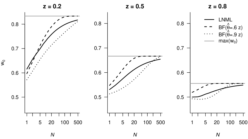
Figure 2: In contrast to LNML, the convergence rate of the Bayes factor to the maximum model weight in favor of the order constraint depends on the exact data if $\hat{\theta}_{y,1}\leq z$. The two Bayes factors shown correspond to data resulting in ML estimates of $\hat{\theta}_{y,1}=0.6z$ and $\hat{\theta}_{y,1}=0.9z$ for all $N$.

In sum, whenever the estimator for the constrained model equals that of the full model (i.e., the order constraint is satisfied), LNML no longer depends on the observed data. In contrast, the Bayes factor remains sensitive to the observed data.

3.2 Model Preference

Figure 3 shows data for which the Bayes factor and LNML prefer a different model. In these cases, LNML selects the constrained model, whereas the Bayes factor based on uniform priors prefers the full model. For a boundary of $z=0.8$, for instance, the Bayes factor sometimes prefers the full model even though the ML estimator satisfies the order constraint. This occurs when the posterior for $\theta$ under $\mathcal{M}_{1}$ has less mass over the range $\theta\leq.8$ than the prior for $\theta$ under $\mathcal{M}_{1}$ (cf. Eq. 5). Figure 4 illustrates this counterintuitive result.

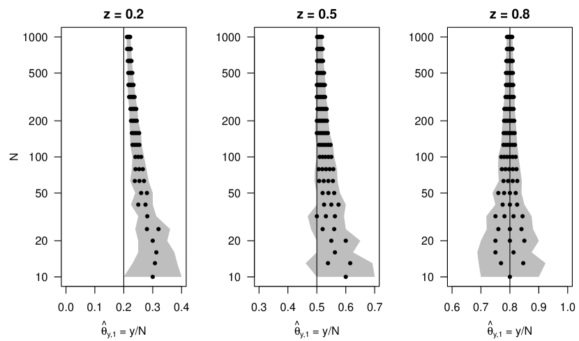
Figure 3: Black dots represent possible data for which LNML prefers the order-constrained model, whereas the Bayes factor favors the full binomial model. The gray area shows divergence in model preference and is bounded to the left and the right by data for which the Bayes factor and LNML agree which model to prefer.

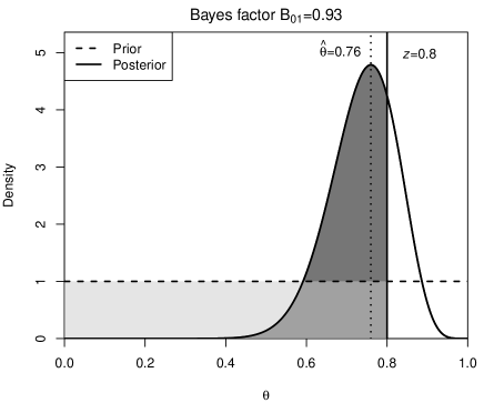
Figure 4: The Bayes factor can prefer the unconstrained model even though the order constraint $\theta\leq z$ is satisfied by the ML estimator ($N=25$, $y=19$). $\text{B}_{01}$ is computed as the ratio of posterior mass (dark gray) to prior mass (light gray) on the order-restricted range $[0,z]$.

The proportion of possible data sets with diverging results increases with $z$. For example, with $N=20$ and $z=0.2$, only $5$% of possible data sets lead to diverging model preferences, increasing to $10$% for $z=0.5$ and $15$% for $z=0.8$. However, for larger sample sizes, the differences in model preference between Bayes factors and LNML decrease; for example, when $N=1000$, the proportions of critical data sets fall to $1.2$%, $1.8$%, and $1.9$%, respectively. Note that in all of these critical cases, the model weights of both methods only show weak preferences for or against the order constraint (i.e., all $w_{0}^{L}<0.77$ and all $w_{0}^{B}>0.16$). Therefore, this qualitative difference might only have minor consequences for model selection in practice.

In sum, for most data sets both LNML and the Bayes factor will prefer the same model even in small samples. However, for ambiguous data where the ML estimator is near the order constraint, LNML and the Bayes factor may prefer different models.

4 Discussion

We identified two qualitative differences between Bayes factors and LNML in testing order constraints, which also apply to standard NML as a special case. First, if the order constraint is satisfied, LNML is independent of the observed data, whereas the Bayes factor remains dependent on the observed data. This implies that the speed of evidence accumulation in favor of an order constraint is constant for LNML, but depends on how well the constraint is satisfied for the Bayes factor. Second, in some cases, the Bayes factor may favor the full model while LNML prefers the constrained model. Whereas the data independence of LNML holds for tests of order constraints in general (cf. Eq. 12), differences in model preference might depend on the exact model. However, we expect that preferences are more likely to differ close to the boundary and decrease for larger samples, similarly as for the binomial model.

One common advantage of Bayes factors and NML concerns their ability to take order constraints into consideration, contrary to model selection tools such as AIC or BIC. Although several authors have stressed the similarities between Bayes factors and NML (e.g., Grünwald, 2007; Bartlett et al., 2013; Kakade et al., 2006), a detailed study of order-constrained inference shows that what is good for belief revision (Bayes) is not necessarily good for data compression (NML).

References

- Bartlett et al. (2013) Bartlett, P., Grünwald, P., Harremoës, P., Hedayati, F., Kotlowski, W., 2013. Horizon-independent optimal prediction with log-loss in exponential families. JMLR: Workshop and Conference Proceedings 30, 639–661.
- Grünwald (2007) Grünwald, P., 2007. The Minimum Description Length Principle. MIT Press, Cambridge, MA.
- Kakade et al. (2006) Kakade, S. M., Seeger, M. W., Foster, D. P., 2006. Worst-case bounds for Gaussian process models. In: Weiss, Y., Schölkopf, B., Platt, J. (Eds.), Advances in Neural Information Processing Systems 18. MIT Press, Cambridge, MA, pp. 619–626.
- Kass and Raftery (1995) Kass, R. E., Raftery, A. E., 1995. Bayes factors. Journal of the American Statistical Association 90, 773–795.
- Klugkist and Hoijtink (2007) Klugkist, I., Hoijtink, H., 2007. The Bayes factor for inequality and about equality constrained models. Computational Statistics & Data Analysis 51, 6367–6379.
- Lewis and Raftery (1997) Lewis, S. M., Raftery, A. E., 1997. Estimating Bayes factors via posterior simulation with the Laplace–Metropolis estimator. Journal of the American Statistical Association 92, 648–655.
- Rissanen (1978) Rissanen, J., 1978. Modeling by shortest data description. Automatica 14, 465–471.
- Rissanen (1996) Rissanen, J., 1996. Fisher information and stochastic complexity. IEEE Transactions on Information Theory 42, 40–47.
- Rissanen (2001) Rissanen, J., 2001. Strong optimality of the normalized ML models as universal codes and information in data. IEEE Transactions on Information Theory 47, 1712–1717.