Getting information via a quantum measurement: the role of decoherence

Abstract

In this work we investigate the relation between quantum measurements and decoherence, in order to formally express the necessity of the latter for obtaining an informative output from the former. To this aim, we analyse the dynamical behaviour of a particular model, which is often adopted in the literature for describing projector valued measures of discrete observables. The analysis is developed by a recently introduced method for studying open quantum systems, namely the parametric representation with environmental coherent states: this method allows us to determine a necessary condition that the evolved quantum state of the apparatus must fulfil in order to have the properties that a measurement scheme requests it to feature. We find that this condition strictly implies decoherence in the system object of the measurement, with respect to the eigenstates of the hermitian operator that represents the measured observable. The relevance of dynamical entanglement generation is highlighted, and consequences of the possible macroscopic structure of the measurement apparatus are also commented upon.

1 Introduction

The profound relation between the quantum measurement process and decoherence is nowadays recognised as a key feature of quantum mechanics, not only from a foundational viewpoint but also when designing theoretical models or experimental setups aimed at capturing genuinely quantum behaviours of physical systems BuschLM96 ; NamikiPascazioNakazato1997 ; Zurek2003 ; Schlosshauer . However, in the formal construction of such relations there are still unclear points, that enforce the introduction of otherwise unnecessary concepts or even of additional axioms. It is not too stretched to say that these unclear points tend to nest where the crossover towards a macroscopic measurement apparatus comes into play and the quantum-to-classical transition consequently bursts into the descriptionBuschLM96 ; Schlosshauer ; GhirardiRW85 ; GhirardiRW86 ; NakazatoP93pra ; Mermin98 . What makes it particularly problematic the formal treatment of such transition, in the specific case of the measurement process, is the fact that it must exclusively concern the apparatus without affecting the object of the measurement, hereafter dubbed principal system, whose quantum character is not at issue. The aim of this work is that of giving a formal content to the role played by decoherence in the way we effectively probe the quantum world.

In the approach to which we will essentially refer, the measurement process is represented as an inherently dynamical one, entailing the definition of what is

-before (the principal system in the state about which we want to acquire information, and the apparatus initialised in some dumb configuration),

-during (the evolution ruled by the measurement coupling that generates entanglement between principal system and apparatus),

- and after (the principal system in some final state and the apparatus in an informative and readable output configuration).

Notice that the above splitting implies the possibility of switching on/off the measurement coupling, a task which is most often accomplished by reducing/increasing, respectively, the distance between systems, with the implicit assumption that only short range interactions are relevant. Consistently, in this work we will not consider long range interactions, such as the Coulomb or gravitational ones.

Collecting clues from the above reflections we propose a description of a specific case of quantum measurement process in terms of the dynamical evolution of an Open Quantum System (OQS)Kraus83 ; Breuer2002 ; Holevo12 ; Rivas2012 whose environment is the measuring apparatus. We resort to a recently introduced methodCalvaniEtal2013b for studying OQS, namely the Parametric Representation with Environmental Coherent States (PRECS), which is specifically tailored to follow the environmental quantum-to-classical crossover. Indeed one of the main feature of the PRECS is that of allowing an exact, and yet essentially asymmetric description of principal system and environment, with the former given in terms of parametrised pure states, and the latter strongly characterised by the use of generalised coherent states.

The structure of the paper is as follows: In Sec.2 we define the specific type of quantum measurement that will be considered, and introduce the model adopted for describing the process in the framework of the OQS dynamics. The resulting evolution is studied in Sec.3 by the PRECS, which is briefly reviewed and commented upon in this same section. The crucial point of how information about the principal system becomes available through the apparatus is finally tackled in Sec.4, where decoherence appears as a necessary phenomenon in order for the measurement process to produce an informative output. Results are commented upon and conclusions drawn in Sec.5.

2 Standard model for unitary pre-measurements of discrete sharp observables

Providing a formal description of the quantum measurement process is a challenge that, despite having been extensively taken on in the last century, cannot yet be considered definitively overcome. Different approaches have been proposed but no general consensus in favour of any of them has been reached (see Refs.BuschLM96 and Schlosshauer for discussions and bibliographies on the subject). Aim of this Section is that of sketching the formalism we will refer toBuschLM96 , and define the specific case we will explicitly study.

Be $\Gamma$ the principal system, object of the measurement, and $\Xi$ its environment, acting as measuring apparatus: both systems are described as quantum ones, with separable Hilbert spaces ${\cal H}_{\Gamma}$ and ${\cal H}_{\Xi}$, respectively. The composite system $\Psi=\Gamma+\Xi$, with separable Hilbert space ${\cal H}_{\Psi}={\cal H}_{\Gamma}\otimes{\cal H}_{\Xi}$, is assumed isolated: its state is therefore pure at any time, $\rho_{\Psi}(t)=|{\Psi(t)}\rangle\langle{\Psi(t)}|~{}\forall t$, and further presumed separable before the measurement starts

$$|{\Psi(t\leq 0)}\rangle=|{\Gamma}\rangle\otimes|{\Xi}\rangle~{};$$ (1)

notice that the validity of these assumptions should not be taken for granted, as extensively discussed, for instance, in Refs.BuschLM96 ; Schlosshauer . The subsystems $\Gamma$ and $\Xi$ are certainly not isolated for $t>0$, and their respective state is $\rho_{\Gamma}(t)={\rm Tr}_{\Xi}[|{\Psi(t)}\rangle\langle{\Psi(t)}|]$, $\rho_{\Xi}(t)={\rm Tr}_{\Gamma}[|{\Psi(t)}\rangle\langle{\Psi(t)}|]$, where ${\rm Tr}_{\Gamma(\Xi)}$ indicates the partial trace over ${\cal H}_{\Gamma(\Xi)}$.

An observable $O_{\Gamma}$ of $\Gamma$ is most generally defined as - and identified with - a positive operator valued measure (POVM) on some measurable space that describes the possible measurement outcome of the observable itself. Multiplicative POVMs can be shown to coincide with projection operator valued measures and, when acting on the real Borel space or a subset of it, define observables that will be hereafter dubbed sharp observablesBuschLM96 . Any such measure determines a unique Hermitian operator ${\hat{O}}_{\Gamma}$ acting on ${\cal H}_{\Gamma}$, and viceversa. If $O_{\Gamma}$ is a discrete sharp observable, the spectral decomposition of the related operator reads

$$\hat{O}_{\Gamma}=\sum_{\gamma,i}\omega_{\gamma}|{\gamma i}\rangle\langle{\gamma i}|~{},$$ (2)

where $\{\omega_{\gamma}\}$ is the set of different $\hat{O}_{\Gamma}$-eigenvalues, with respective degeneracy ${\rm d}_{\gamma}$, the multiple index $\gamma i$ runs from $\gamma 1$ to $\gamma{\rm d}_{\gamma}$, and the $\hat{O}_{\Gamma}$-eigenvectors $\{|{\gamma i}\rangle\}$ form an orthonormal basis for ${\cal H}_{\Gamma}$.

Further ingredients of a scheme designed for describing the measure of $O_{\Gamma}$ are i) a pointer observable $O_{\Xi}$ of $\Xi$, to be correlated with $O_{\Gamma}$, ii) a pointer function $f$ correlating the value sets of $O_{\Xi}$ and $O_{\Gamma}$, iii) a measurement coupling $V$ between $\Gamma$ and $\Xi$, ultimately responsible for the $\Psi$-state transformation $\rho_{\Psi}(0)\xrightarrow{V}\rho_{\Psi}(t)$ occurring during the preliminary stage of the process, i.e. before the actual production of a specific outcome is obtained. In order to define a measurement scheme, a state transformation must feature some specific properties; most importantly it must guarantee that the probability reproducibility condition holds, i.e. that

$${\rm p}^{O_{\Gamma}}_{\rho_{\Gamma}(0)}(\omega_{\gamma}) = {\rm p}^{O_{\Xi}}_{\rho_{\Xi}(t)}(f^{-1}(\omega_{\gamma}))$$ (3)

$$\forall\omega_{\gamma}~{}{\rm in~{}the~{}set}~{}\{\omega_{\gamma}\} {\rm and} {\rm for~{}all~{}possible~{}}\rho_{\Gamma}(0)~{},$$

where p${}^{O_{\Gamma}}_{\rho_{\Gamma}(0)}(\omega_{\gamma})$ is the probability measure for the value $\omega_{\gamma}$ of $O_{\Gamma}$ when $\Gamma$ is in the state $\rho_{\Gamma}(0)$, and p${}^{O_{\Xi}}_{\rho_{\Xi}(t)}(f^{-1}(\omega_{\gamma}))$ is that for the value $f^{-1}(\omega_{\gamma})$ of $O_{\Xi}$ when $\Xi$ is in the state $\rho_{\Xi}(t)={\rm Tr}_{\Gamma}[V[\rho_{\Psi}(0)]]$. Although discussing the meaning and relevance of condition (3) goes beyond the purpose of this work, we notice the following: The Shannon entropy associated to the distribution of probability measures p${}^{O_{\Gamma}}_{\rho_{\Gamma}(0)}$ on the discrete set $\{\omega_{\gamma}\}$ is interpreted, from an information-theoretical viewpoint, as the average deficiency of information on the observable $O_{\Gamma}$ of $\Gamma$ before the measurement starts $(t=0)$. On the other hand, requiring that equality (3) hold, ensures that the above deficiency equals the potential information gain upon measuring the observable $O_{\Xi}$ of $\Xi$, which corresponds to the naive notion that measuring implies information gain. In fact Eq. (3), with its left- and right-hand side referring to $\Gamma$ and $\Xi$, respectively, formally represents an information flow from the principal system to the apparatus: however, despite this information transfer occur whenever $V$ generates entanglement between $\Gamma$ and $\Xi$, in Sec. 4 we will show that decoherence has an essential role in guaranteeing that $t$ be such that the amount of information actually transferred, quantified by the above Shannon entropy, be different from zero. Notice that the distribution of probability measures p${}^{O_{\Xi}}_{\rho_{\Xi}(t)}$ on the set $\{f^{-1}(\omega_{\gamma})\}$ can be obtained by reconstructing the state $\rho_{\Xi}(t)$ by quantum tomographyDarianoL-P01 ; DarianoMP00 , i.e. by determining the expectation values ${\rm Tr}[\hat{Z}^{I}_{\Xi}\rho_{\Gamma}(t)]$ of an appropriate set $\{Z^{I}_{\Xi}\}$ of observables on $\Xi$.

Getting back to the measurement scheme, it can be shown that a sufficient condition for a state transformation to qualify as a proper pre-measurement, by this meaning that it fulfils Eq. (3), is that $V$ be a trace-preserving linear mapping. When $V$ is further assumed to be unitary, the process coincides with the one first described by von NeumannNeumann1996 , later generalised by several authorsLondonB39 ; Wigner52 ; ArakiY60 ; Yanase61 ; ShimonyS71 ; ShimonyS79 ; Busch87 ; BuschS89 and characterised in Ref. Ozawa84 under the name of conventional measuring process.

The pre-measurement step of this type of process is defined by a unitary operator ${\hat{U}}$ on ${\cal H}_{\Psi}$ satisfying

$$\hat{U}(|{\gamma i}\rangle\otimes|{\Xi}\rangle)=\sum_{j}|{\gamma j}\rangle\otimes|{\Xi^{\gamma}}\rangle~{},$$ (4)

for any $\gamma,i$. Notice that, as we are not measuring the degeneracy parameter $i$, Eq. (4) allows the possibility that $\Gamma$ remain in any state of the $\hat{O}_{\Gamma}$-invariant subspace of ${\cal H}_{\Gamma}$ corresponding to the eigenvalue $\omega_{\gamma}$. If $O_{\Xi}$ is a sharp observable, with $\hat{O}_{\Xi}$ the corresponding hermitian operator, the propagator

$$\hat{U}_{\tau}\equiv e^{-i\frac{\tau}{\hbar}\hat{H}_{\Psi}}$$ (5)

with

$$\hat{H}_{\Psi}=g\hat{O}_{\gamma}\otimes\hat{O}_{\Xi}+\hat{\mathbf{1}}_{\Gamma}\otimes\hat{H}_{\Xi}~{},$$ (6)

where $\hat{H}_{\Xi}$ acts on ${\cal H}_{\Xi}$ and $\hat{\mathbf{1}}_{\Gamma}$ is the identity operator on ${\cal H}_{\Gamma}$, defines a model, referred to as the standard model BuschLM96 , for properly describing unitary pre-measurements as dynamical processes.

In what follows we will specifically study the standard model for the unitary pre-measurement of a discrete sharp observable and, for the sake of simplicity, we will further assume such observable to be non-degenerate. As for the parameter $\tau$ in Eq.(5), we identify it with the time $t$.

Writing $|{\Gamma}\rangle$ in Eq. (1) on the basis of the $\hat{O}_{\Gamma}$-eigenstates, from Eqs. (5-6) it follows

$$|{\Psi(t)}\rangle=\sum_{\gamma}c_{\gamma}|{\gamma}\rangle\otimes|{\Xi^{\gamma}(t)}\rangle~{}$$ (7)

at any time during the pre-measurement process, with

$$|{\Xi^{\gamma}(t)}\rangle\equiv e^{-i\frac{t}{\hbar}\hat{H}^{\gamma}}|{\Xi}\rangle~{},$$ (8)

and $\hat{H}^{\gamma}\equiv g\omega_{\gamma}\hat{O}_{\Xi}+\hat{H}_{\Xi}$. The density operator for $\Gamma$ consequently reads

$$\rho_{\Gamma}(t)=\sum_{\gamma}|c_{\gamma}|^{2}|{\gamma}\rangle\langle{\gamma}|+\sum_{\gamma\neq\gamma^{\prime}}c_{\gamma}c^{*}_{\gamma^{\prime}}\langle{\Xi^{\gamma^{\prime}}(t)|\Xi^{\gamma}(t)}\rangle|{\gamma}\rangle\langle{\gamma^{\prime}}|~{},$$ (9)

showing that, due to the structure of $\hat{H}_{\Psi}$, only the off-diagonal elements of the above representation of $\rho_{\Gamma}$ evolve in time (which is why this type of evolution has been recently dubbed ”off-diagonal dynamics”Calvani2013 ). It is of absolute relevance, as it will further result in Sec.3, that the evolution of $\rho_{\Gamma}$ is exclusively ruled by the time dependence of the overlaps $\langle{\Xi^{\gamma^{\prime}}(t)|\Xi^{\gamma}(t)}\rangle$.

3 Off-diagonal dynamics by the PRECS

Our next step is that of obtaining an expression for $\rho_{\Gamma}(t)$ that allow us to go beyond the pre-measurement stage. To this aim we resort to the parametric representation with environmental coherent states (PRECS): the method has been recently introducedCalvaniEtal2013b as a tool for studying OQS with an environment that needs being considered quantum, but yet may have an extremely large Hilbert space. It is based on the construction of generalised coherent statesZhangFG1990 ; Perelomov1972 for the environment, or environmental coherent states (ECS), relative to the group, usually referred to as ”dynamical group”, in terms of whose generators one can write the operators $\hat{O}_{\Xi}$ and $\hat{H}_{\Xi}$ in $\hat{H}_{\Psi}$. Without entering into the details of their construction and propertiesComberscue2012 , we recall that ECS, hereafter indicated by $|{\Omega}\rangle$, form an overcomplete set on ${\cal H}_{\Xi}$ and are in one-to-one correspondence with points $\Omega$ on a differentiable manifold ${\cal M}$. This correspondence is strictly local, but coherent states are not orthogonal due to their overcompleteness, which suggests that they can be used also for studying pre-measurements where $O_{\Xi}$ is a POVM. On the other hand, and this is just one of the many ECS properties that make them the ideal tool for investigating the quantum to classical transition, their overlaps exponentially vanish as dim${\cal H}_{\Xi}$ grows, and the manifold ${\cal M}$ is demonstrated to be a proper phase-space in the classical limitYaffe1982 .

The construction of ECS requires the (arbitrary) choice of a reference state $|{R}\rangle\in{\cal H}_{\Xi}$, whose representative point will define the origin of the reference frame on ${\cal M}$; the procedure entails the definition of an invariant (with respect to the dynamical group) measure $d\mu(\Omega)$ on ${\cal M}$, as well as a metric tensor ${\bf m}$. ECS provide an identity resolution on ${\cal H}_{\Xi}$ in the form

$$\hat{\mathbf{1}}_{\mathcal{H}_{\Xi}}=\int_{\cal M}\,d\mu(\Omega)|{\Omega}\rangle\langle{\Omega}|~{}.$$ (10)

Due to their being constructed in relation to the dynamical group, coherent states have peculiar dynamical properties, which are often summarised by the motto ”once a coherent state, always a coherent state”ZhangFG1990 . Referring to our specific setup, if the initial state of the apparatus is a coherent state, from Eq. (8) it follows

$$|{\Xi^{\gamma}(t)}\rangle=e^{i\varphi^{\gamma}_{t}}|{\Omega^{\gamma}_{t}}\rangle~{},$$ (11)

with

• $|{\Omega^{\gamma}_{t}}\rangle$ the coherent state corresponding to the point $\Omega(t)$ on the trajectory on ${\cal M}$ defined by the solution of the classical-like equations of motion

  $$i{\bf m}\frac{d\Omega}{dt}=\frac{\partial}{\partial\Omega^{*}}H^{\gamma}(\Omega)~{}~{}~{}{\rm and~{}c.c.}~{},\$$ (12)

  with $H^{\gamma}(\Omega)=\langle{\Omega|\hat{H}^{\gamma}|\Omega}\rangle$,

• and

  $$\varphi^{\gamma}_{t}=\int_{0}^{t}~{}dy\langle{\Omega^{\gamma}_{y}|\left(i\frac{\partial}{\partial y}-\hat{H}^{\gamma}\right)|\Omega^{\gamma}_{y}}\rangle~{}.$$ (13)

Getting back to our composite system $\Psi$, once ECS are constructed, its subsystems $\Gamma$ and $\Xi$ can be formally split by inserting ${\mathbf{1}}_{{\cal H}_{\Xi}}$ as from Eq. (10) into any state $|{\Psi}\rangle$, including one written in the form (7). In particular, choosing the initial state of the measuring apparatus as the reference state for the ECS construction, $|{R}\rangle=|{\Xi}\rangle$, and exploiting the fact that $d\mu(\Omega)$ is group-invariant, we can write

$$|{\Psi(t)}\rangle=\int_{\cal M}~{}d\mu(\Omega)\chi_{t}(\Omega)|{\phi_{t}(\Omega)}\rangle|{\Omega}\rangle~{},$$ (14)

with

$$|\phi_{t}(\Omega)\rangle = \frac{1}{\chi_{t}(\Omega)}\sum_{\gamma}c_{\gamma}\langle{\Omega|R^{\gamma}_{t}}\rangle|{\gamma}\rangle~{},$$ (15)

$$\chi_{t}(\Omega) = \sqrt{\sum_{\gamma}|c_{\gamma}|^{2}h^{\gamma}_{t}(\Omega)}~{},$$ (16)

$$h^{\gamma}_{t}(\Omega) = |\langle{\Omega|R^{\gamma}_{t}}\rangle|^{2}~{},$$ (17)

where $|{R^{\gamma}_{t}}\rangle$ is the coherent state corresponding to the point $R^{\gamma}(t)$ on the trajectory defined by the solution of Eq. (12) with initial condition $\Omega(0)=0$, and we have set $\chi_{t}(\Omega)$ in ${R}^{+}$ by choosing its arbitrary phase equal to $0$. Due to $\langle{\Psi(t)|\Psi(t)}\rangle=1$ at any time, it is

$$\int_{\cal M}d\mu(\Omega)\chi^{2}_{t}(\Omega)=1~{}~{}~{}\forall t~{}.$$ (18)

The above Eqs.(14-17) define the parametric representation with environmental coherent states of $|{\Psi(t)}\rangle$. It can be shownZhangFG1990 ; CalvaniEtal2013b that corresponding form for $\rho_{\Gamma}(t)$ is

$$\rho_{\Gamma}(t)=\int_{\cal M}d\mu(\Omega)\chi^{2}_{t}(\Omega)|{\phi_{t}(\Omega)}\rangle\langle{\phi_{t}(\Omega)}|~{},$$ (19)

suggesting that $\chi^{2}_{t}(\Omega)$ can be interpreted, consistently with Eq. (18), as the density distribution of ECS on ${\cal M}$. To this respect it is worth noticing that $\chi^{2}_{t}(\Omega)=\langle{\Omega|\rho_{\Xi}(t)|\Omega}\rangle$.

4 Extracting information from the apparatus: emergence of decoherence

The description of the standard model for unitary pre-measurements of discrete, non degenerate, sharp observables by the PRECS essentially amounts to express $\rho_{\Gamma}(t)$, as from Eq. (9), in the form (19), with $\chi^{2}_{t}(\Omega)=\sum_{\gamma}|c_{\gamma}|^{2}h_{t}^{\gamma}(\Omega)$ and the initial state of the measuring apparatus chosen as reference state for constructing ECS. In fact, by comparing Eqs. (9) and (19), it might seem that we ended up with having overturned the dependencies with respect to the scheme (4), as Eq. (19) shows that $|\phi_{t}(\Omega)\rangle$ depends on the environmental parameter $\Omega$, while the coherent state $|{\Omega}\rangle$ of the measuring apparatus is not marked by the label “$\gamma$”. This is because the signature of the interaction with $\Gamma$ is not in the ECS, that are defined independently of $O_{\Gamma}$, but rather in their density distribution $\chi_{t}^{2}(\Omega)$, which is where one should therefore look into, in order to extract information on $\Gamma$ via $\Xi$.

Let us now leave the pre-measurement process and consider the actual production of an outcome. Distinct coherent states, corresponding to distinct states of the measurement apparatus, will produce different outcomes, whose distribution will thus be associated with $\chi^{2}_{t}(\Omega)$. On the other hand, in order for this setup to produce an outcome with some informational content, it is necessary that the $\gamma-$components entering $\chi^{2}_{t}(\Omega)$, i.e. the terms $|c_{\gamma}|^{2}h_{t}^{\gamma}(\Omega)$, be sufficiently separated from each other to be distinguishable. Aiming at formally expressing this condition, let us consider the functions $h^{\gamma}_{t}(\Omega)$ in Eq. (17): They are normalised distributions on ${\cal M}$ whose $\varepsilon$-support, defined as the region $S^{\gamma}_{t}\in{\cal M}$ such that $h^{\gamma}_{t}(\Omega)>\varepsilon~{}\forall\Omega\in S^{\gamma}_{t}$ (with $\varepsilon$ a reasonably small number in ${\mathbf{R}}^{+}$), moves on such manifold with time. If, after some time, we have

$$S^{\gamma}_{t}\cap S^{\gamma^{\prime}}_{t}=\emptyset~{},~{}\forall\gamma\neq\gamma^{\prime}~{},$$ (20)

then each distribution $h^{\gamma}_{t}$ can be individually located, and a one-to-one correspondence between the label $\gamma$ and the region $S^{\gamma}_{t}$ on ${\cal M}$ is established. Notice that a weaker condition $(\cup_{i\in{\cal I}}S^{\gamma_{i}}_{t})\cap(\cup_{j\in{\cal J}}S^{\gamma^{\prime}_{j}}_{t})=\emptyset$ would also establish a correspondence, although of a many-to-one type. However, for the sake of clarity, in what follows we will concentrate upon the strong distinguishability condition (20), identifying it with that guaranteeing that an informative output can be extracted from the apparatus. This finally brings us to the question we aimed at answering: how and why this condition, that somehow regards $\Xi$ only, is related with the occurrence of decoherence in the principal system $\Gamma$? In order to take this last step forward, consider Eq. (9): If condition (20) holds, we have

$$\rho_{\Gamma}(t) {\approx} \sum_{\gamma}|c_{\gamma}|^{2}\int_{S^{\gamma}_{t}}~{}d\mu(\Omega)h^{\gamma}_{t}(\Omega)|{\phi(\Omega,t)}\rangle\langle{\phi(\Omega,t)}|$$ (21)

$${=} \sum_{\gamma}|c_{\gamma}|^{2}|{\gamma}\rangle\langle{\gamma}|~{},$$

that exactly expresses the vanishing of the off-diagonal elements of $\rho_{\Gamma}$ on the $\{|{\gamma}\rangle\}$ basis, i.e. the formal definition of decoherence for the principal system $\Gamma$. This makes finally evident that decoherence is not one of the many byproducts of the measurement process, but rather a necessary condition for the configuration of the apparatus to embody some usable information on $\Gamma$.

In order to better understand the construction that brought us to the above result, let us consider a simple example. Take $\Gamma$ as a quantum system with ${\rm dim}{\cal H}_{\Gamma}=2$ (usually referred to as qubit), and $\Xi$ as a single-mode bosonic field. Be the Hamiltonian

$$\hat{H}=g\sqrt{\hbar}\sigma^{z}(b+b^{\dagger})+\nu b^{\dagger}b~{},$$ (22)

with $[b,b^{\dagger}]=\hbar$, $[\sigma^{\alpha},\sigma^{\beta}]=i\varepsilon^{\alpha\beta\delta}{\sigma}^{\delta}$, $\alpha(\beta,\delta)=x,y,z$, and ${\vec{\sigma}}$ the Pauli operator. The above Hamiltonian is in the form (6) and the corresponding ECS, taking the reference state $|{R}\rangle$ such that $b|{R}\rangle=0$, are the usual field coherent states, with ${\cal M}$ the complex plane, ${\rm d}\mu=d\Omega d\Omega^{*}/(\pi\hbar)$ the invariant measure, and ${\bf m}=\hbar^{-1}$ the (diagonal) metric tensor. Being ${\rm dim}{\cal{H}}_{\Gamma}=2$, the label $\gamma$ can only take two values, hereafter indicated by $\pm$, and the initial state $\Gamma$ can be written as $(c_{+}|{+}\rangle+c_{-}|{-}\rangle)$, where $|{\pm}\rangle$ are the eigenstates of $\sigma^{z}$. Solutions of Eq. (12) are two circles $R^{\pm}_{t}(\Omega)$ on the ${\rm Re}(\Omega)-{\rm Im}(\Omega)$ plane, passing through $(0,0)$, centred in $(\mp g/\nu,0)$, and gone through clockwise.

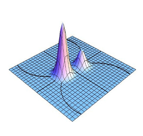
Figure 1: Distribution $\chi^{2}_{t}(\Omega)$ at $t=\pi/30$ for the qubit-boson model, Eq. (22), with $g\sqrt{\hbar}=2$ and $\nu=1$. In the initial state of the qubit it is $|c_{+}|^{2}=1/4$ and $|c_{-}|^{2}=3/4$

A snapshot of the ECS density distribution $\chi^{2}_{t}(\Omega)$ on the complex plane is shown in Fig. 1, together with part of the orbits $R^{\pm}_{t}(\Omega)$: the two components $|c_{\pm}|^{2}h^{\pm}_{t}(\Omega)$ are already distinguishable, with the respective $\varepsilon$-supports $S^{\pm}_{t}$ quite well separated. Notice that, despite this image portrays the environment $\Xi$, it also mirrors the structure of the principal system state, $\rho_{\Gamma}$, due to the relation between condition (20) and Eq. (21). Although we have never mentioned it so far, it is worth noticing that the above relation between distinguishability of different $h^{\gamma}_{t}$ and diagonal form of $\rho_{\Gamma}(t)$ is established by the entanglement generation entailed by a non-trivial dynamical evolution of $\Psi$, such as that resulting from the interaction (6).

The idea that the ECS distribution $\chi^{2}_{t}(\Omega)$ be the “image” from which we can extract information on $\Gamma$ can be made more precise by introducing the differential entropy for $\chi^{2}_{t}(\Omega)$

$$\mathcal{E}(t) = -\int_{\cal M}d\mu(\Omega)\chi^{2}_{t}(\Omega)\log\chi^{2}_{t}(\Omega)=$$ (23)

$$= -\sum_{\gamma}\int_{\cal M}d\mu(\Omega)|c_{\gamma}|^{2}h_{t}^{\gamma}(\Omega)\log\left(\sum_{\gamma}|c_{\gamma}|^{2}h_{t}^{\gamma}(\Omega)\right)~{}.$$ (24)

Referring to our example Eq. (22), the explicit form of the distributions $h^{\pm}_{t}(\Omega)$ is

$$h_{t}^{\pm}(\Omega)=\frac{1}{\pi\hbar}|\langle\Omega|R_{t}^{\pm}\rangle|^{2}=\frac{1}{\pi\hbar}e^{-\frac{1}{\hbar}|\Omega-R_{t}^{\pm}|^{2}}~{},$$ (25)

corresponding to gaussians centred in $R^{\pm}_{t}$ with constant variance $\hbar$. As the orbits $R^{\pm}_{t}$ initially coincide, it exists an early stage of the process, no matter the coefficients $c_{\pm}$, during which $\chi^{2}_{t}(\Omega)$ keeps being an essentially uni-modal distribution, centred in the origin of the complex plane, which implies $\mathcal{E}\sim\mbox{const}$, with no dependence on $c_{\pm}$, whatsoever. On the other hand, the trajectories $R^{\pm}_{t}$ dynamically separate from each other and, after a certain time, condition (20) starts holding, and the entropy

$$\mathcal{E}\sim-\sum_{\gamma=\pm}|c_{\gamma}|^{2}\int_{S^{\gamma}_{t}}d\Omega d\Omega^{*}h_{t}^{\gamma}(\Omega)\log\left(|c_{\gamma}|^{2}h_{t}^{\gamma}(\Omega)\right)$$ (26)

is seen to depend on the coefficients $|c_{\pm}|^{2}$, and to quantify the amount of information on the state $\Gamma$ that we can obtain adopting a measurement scheme based on the coupling (22). Fig.2 offers a visual rendering of the above result via the contour plot of $\chi^{2}_{t}(\Omega)$ on the complex plane at different times: it is evident that the information content of the initial plot has nothing to do with the state of the principal system $\Gamma$, while the later emergence of two distinct fuzzy spots can be used to extract data on $c_{+}$ and $c_{-}$.

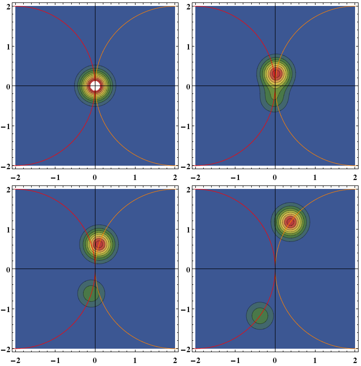
Figure 2: Contour-plot of $\chi^{2}_{t}(\Omega)$ at $t=0,~{}\pi/20,~{}\pi/10,~{}\pi/5$, (panels $A,~{}B,~{}C,~{}D$, resp.), with other parameters as in Fig.1 . Different colours refer to different values of $\chi^{2}_{t}(\Omega)$, increasing from blue ($\chi^{2}_{t}(\Omega)\sim 0$) to white.

5 Conclusions

The analysis presented in this work formally shows that the reason why decoherence of the principal system is a necessary ingredient of a significant measurement process is that the information content of the apparatus would be otherwise null. To this respect it is important to recall that decoherence is defined as the dynamical process causing the vanishing of the off-diagonal elements of the system’s density matrix, with respect to a precise basis on its Hilbert space. When considering the measurement process of a sharp observable, the relevant decoherence phenomenon is just that relative to the basis of eigenstates for the hermitian operator describing the observable itself. In fact, such basis explicitly comes into play when designing the interaction between principal system and apparatus, which is ultimately responsible for the information flow between the twos. Indeed, what does not depend on the specific observable to be measured, is the essential role of the dynamical entanglement generation, without which there would be no correlation between $\Gamma$ and $\Xi$ capable of leaving on the latter any trace of the quantum state of the former. This is an essential feature of quantum measurement, that accounts for the inability of approaches based on classical-like treatments of $\Xi$ to describe quantum measurements, as there cannot be entanglement between a quantum system to be observed and a classical apparatus that makes the measuring.

The necessary condition that both $\Gamma$ and $\Xi$ be quantum systems, on the other hand, raises another question worth being considered, namely whether one should expect coherence to be restored after a certain time or not. In fact, being $\Psi$ a quantum system, and its dynamics unitary, the evolution of both $\Gamma$ and $\Xi$ are superpositions of periodic motions, so that the time interval during which the apparatus is capable of conveying information is in principle finite. However, it can be shownYaffe1982 ; Lieb1973 that when the dimension of the environmental Hilbert space grows, reflecting the fact that the apparatus is macroscopic, the environmental distributions $h^{\gamma}_{t}(\Omega)$ tend to Dirac $\delta$-functions and the recurrence time, i.e. the period of the unitary dynamics, diverges: as a consequence, decoherence occurs after an infinitesimally small time $\tau$, and coherence is never restored. To this respect, we underline that we have not considered the very last stage of the measurement process, where the Born’s rule and the ”wave-function collapse” come into play, and the unitarity of dynamics is lost. However, we believe the PRECS formalism, can give original clues also with respect to these fundamental issues, but we postpone their possible analysis to future works. Moreover, although we have restricted ourselves to a particular model that describes only a specific type of measurement, the present analysis might be useful also for treating more general situations.

6 Acknowledgements

This work has been done in the framework of the Convenzione operativa between the Institute for Complex Systems of the italian National Research Council, and the Physics and Astronomy Department of the Univeristy of Florence.

References

- (1) P. Busch, J.P. Lathi, P. Mittelstaedt, The quantum theory of measurement (Springer-Verlag, Berlin, 1996).
- (2) M. Namiki, S. Pascazio, H. Nakazato, Decoherence and Quantum Measurements (World Scientific, 1997).
- (3) W.H. Zurek, Rev. Mod. Phys. 75, 715 (2003).
- (4) M. Schlosshauer, Decoherence and the Quantum-To-Classical Transition. The Frontiers Collection (Springer, 2007).
- (5) G. Ghirardi, A. Rimini, T. Weber, in Quantum Probability and Applications, L. Accardi et al. (eds) (1985).
- (6) G. Ghirardi, A. Rimini, T. Weber, Phys. Rev. D 34, 470 (1986).
- (7) H. Nakazato, S. Pascazio, Phys. Rev. A 48, 1066 (1993).
- (8) D. Mermin, American Journal of Physics 66, 753 (1998).
- (9) K. Kraus, States, Effects, and Operations (Springer-Verlag, Berlin, 1983).
- (10) H.P. Breuer, F. Petruccione, The theory of open quantum systems (Oxford University Press, 2002).
- (11) A.S. Holevo, Quantum systems, channels, information: a mathematical introduction, vol. 16 (Walter de Gruyter, 2012).
- (12) A. Rivas, S.F. Huelga, Open Quantum Systems: An Introduction (Springer Berlin Heidelberg, 2012).
- (13) D. Calvani, A. Cuccoli, N.I. Gidopoulos, P. Verrucchi, Proceedings of the National Academy of Sciences 110(17), 6748 (2013).
- (14) G.M. D’Ariano, P. Lo Presti, Phys. Rev. Lett. 86, 4195 (2001).
- (15) G.M. D’Ariano, L. Maccone, M.G.A. Paris, Phys. Lett. A 276, 25 (2000)
- (16) J. von Neumann, Mathematical Foundations of Quantum Mechanics (Princeton University Press, 1996) Translation from German.
- (17) F. London, E. Bauer, La teorie de l’observation en mecanique quantique (Herman et cie, 1939).
- (18) E. Wigner, Z. Phys. 133, 101 (1952).
- (19) H. Araki, M.M. Yanase, Phys. Rev. 120, 622 (1960).
- (20) M.M. Yanase, Phys. Rev. 123, 666 (1961).
- (21) A. Shimony, H. Stein, in Foundations of Quantum Mechanics, pp. 56–76 , ed. by B. D’Espagnat (Acad. Press., N. Y., 1971).
- (22) A. Shimony, H. Stein, Am. Math. Mon. 86, 292 (1979).
- (23) P. Busch, Foundations of Physics 17(9), 905 (1987).
- (24) P. Busch, J. Schroeck, Foundations of Physics 19(7), 807 (1989).
- (25) M. Ozawa, J. Math. Phys. 25, 292 (1984)
- (26) D. Calvani, A. Cuccoli, N.I. Gidopoulos, P. Verrucchi, Open Syst. Inform. Dynam. 20(3) (2013)
- (27) W.M. Zhang, D.H. Feng, R. Gilmore, Rev. Mod. Phys. 62, 867 (1990).
- (28) A. Perelomov, Communications in Mathematical Physics 26(3), 222 (1972).
- (29) M. Comberscue, D. Robert, Coherent States and Application in Mathematical Physics (Springer Berlin Heidelberg, 2012).
- (30) L.G. Yaffe, Rev. Mod. Phys. 54, 407 (1982).
- (31) E.H. Lieb, Communications in Mathematical Physics 31(4), 327 (1973).