Searching for tidal tails around $\omega$ Centauri using RR Lyrae Stars

We present a survey for RR Lyrae stars in an area of 50 deg² around the globular cluster $\omega$ Centauri, aimed to detect debris material from the alleged progenitor galaxy of the cluster. We detected 48 RR Lyrae stars of which only 11 have been previously reported. Ten among the eleven previously known stars were found inside the tidal radius of the cluster. The rest were located outside the tidal radius up to distances of $\sim 6$ degrees from the center of the cluster. Several of those stars are located at distances similar to that of $\omega$ Centauri. We investigated the probability that those stars may have been stripped off the cluster by studying their properties (mean periods), calculating the expected halo/thick disk population of RR Lyrae stars in this part of the sky, analyzing the radial velocity of a sub-sample of the RR Lyrae stars, and finally, studying the probable orbits of this sub-sample around the Galaxy. None of these investigations support the scenario that there is significant tidal debris around $\omega$ Centauri, confirming previous studies in the region. It is puzzling that tidal debris have been found elsewhere but not near the cluster itself.

1 Introduction

The globular cluster $\omega$ Centauri is the most massive (Meylan 1987; Meylan et al. 1995; Merritt et al. 1997) among the 157 globular clusters known around the Milky Way. It has several unusual properties that have led to the proposal that the cluster is the remaining core of a dwarf galaxy destroyed due to gravitational interaction with the Milky Way (Bekki & Freeman 2003; Mizutani et al. 2003; Ideta & Makino 2004; Tsuchiya et al. 2004; Majewski et al. 2012). Some of these unusual properties are: (i) a retrograde, low inclination orbit around the Milky Way (Dinescu et al. 1999), (ii) an overall rapid rotation of 7.9 km s^-1(Merritt et al. 1997), making it one of the most flattened galactic globular clusters (White & Shawl 1987), (iii) a color-magnitude diagram showing a complex stellar population, with a wide range of metallicities, two main sequences (Bedin et al. 2004; Sollima et al. 2007), three red giant branches, and an age spread of $\sim$3-6 Gyr between the metal-poor and the most metal-rich populations (Hilker et al. 2004; Sollima et al. 2005), (iv) a complex chemical pattern (King et al. 2012; Gratton et al. 2011; Marino et al. 2012), and (v) a high velocity dispersion measured toward the center of the cluster, which has been interpreted as an indication of having an intermediate mass black hole (Noyola et al. 2010; Anderson & van der Marel 2010; Miocchi 2010; Jalali et al. 2012). It has been proposed that $\omega$ Centauri may be the equivalent to the M54 $+$ Sagittarius dwarf system but, in the case of $\omega$ Centauri, the progenitor galaxy must have been already completely destroyed by now (Carretta et al. 2010). Bekki & Freeman (2003) proposed a self-consistent dynamical model in which $\omega$ Centauri is the nucleus of a nucleated dwarf galaxy that was tidally destroyed when it merged with the first generation of the Galactic thin disk.

The search for remains of the alleged progenitor has not been without controversy. Although Leon et al. (2000) found significant tidal tails coming out of the globular cluster $\omega$ Centauri, other work give opposite results. Leon et al. (2000) used wide-field multi-color images to do star counts around the cluster. They found $\sim 7000$ stars localized outside of the tidal radius of $r_{t}=45$ arcmin (Trager et al. 1995) located along two tidal tails coming from the cluster from opposite directions, and aligned with the tidal field gradient, suggesting they are the result of a collision with the Galactic disk. Their results, however, may have been affected by reddening which may be high and variable around the cluster (Law et al. 2003).

On the other hand, Da Costa & Coleman (2008) made an extensive spectroscopic survey of 4105 stars of the lower red giant branch in the vicinity of the cluster (a region of 2.4 $\times$ 3.9 deg²). Only six of those red giant branch candidates had a velocity consistent with the radial velocity of cluster of ($+$232.2$\pm$0.7) km s^-1 (Dinescu et al. 1999). Da Costa & Coleman (2008) concluded that these stars represent less than 1% of the mass present in the cluster and hence, they do not provide a significant evidence of an extra-tidal population associated with $\omega$ Centauri. This would have been expected if most of the tidal stripping in the progenitor galaxy occurred a long time ago, which is the interpretation given by those authors to their results.

Interestingly, the search for $\omega$ Centauri debris seems to have been more successful in the solar neighborhood by the recognition that stars in the Kapteyn group have kinematics and chemical abundance patterns similar to $\omega$ Centauri (Wylie-de Boer et al. 2010). The chemical pattern was also key for the association of several red giants with retrograde orbits studied by Majewski et al. (2012). Indeed, these authors suggest that $\omega$ Centauri is responsible for most of the red giants in retrograde orbits in the inner halo.

Besides these successful identification of debris, one would like to, ideally, trace debris along other parts of the orbit as well, and most especially near the cluster itself in order to understand better the origin of $\omega$ Centauri. Since $\omega$ Centauri has a rich population of RR Lyrae stars (Kaluzny et al. 2004; Del Principe et al. 2006; Cacciari et al. 2006; Weldrake et al. 2007), as all satellite galaxies of the Milky Way do (see for example, Vivas & Zinn 2006), it is expected that any tidal debris from $\omega$ Centauri would also contain this type of star. The use of RR Lyrae stars as tracers of debris around the cluster has several advantages. They are bright stars which are relatively easy to spot at different distances because of their variability properties. They are standard candles and hence we can identify possible debris as stars at the same distance as the cluster. Finally, they are an old population and hence we expect no contamination by the thin disk (although we still have to deal with thick disk contamination). Extensive previous work have demonstrated that RR Lyrae stars are excellent tracers of substructures in the Halo (Vivas & Zinn 2006; Watkins et al. 2009; Drake et al. 2013, among others). We present here a survey for RR Lyrae stars in a region of $\sim 50$ deg² around $\omega$ Centauri. Preliminary results of this survey were presented in Fernández Trincado et al. (2013).

In Section 2, we describe the observations. The methods for selecting variable stars of the RR Lyrae type are presented in Section 3. The properties, distances and spatial distribution of the RR Lyrae stars detected in this work are discussed in the Section 4. Section 5 analyzes the likelihood that these RR Lyrae stars are part of debris from the destroyed progenitor galaxy of $\omega$ Cen. Finally, conclusions are presented in Section 6.

2 Observations

The techniques used for this survey are similar to the ones used extensively by our group in studies of RR Lyrae stars in the galactic halo and the Canis Major over-density with the QUEST camera (Vivas et al. 2004; Mateu et al. 2009). The photometric survey was carried out using the QUEST camera at the 1.0m Jürgen Stock telescope (1.5m Schmidt Camera) at the National Astronomical Observatory of Llano del Hato, Venezuela. The QUEST camera is a mosaic of 16 CCDs, with a field of view of 2.3$\times$2.5 deg². Each detector has 2048$\times$2048 pixel of 15 $\mu$m, resulting in an angular resolution of 1 arcsec/pix (Baltay et al. 2002).

For the present survey, half of the camera (8 CCDs) was covered with V filters and the other half with I filters. Although the QUEST camera was designed to work more efficiently in drift scan mode near the equator, the high declination of $\omega$ Centauri required to work in a classical point-and-stare mode. An inconvenience of this method is that it is not possible to cover the whole focal plane with the same filter. Hence, appropriate offsets have to be made in order to have uniform covering of the same area of the sky in more than one filter (at any pointing, half of the camera is observing through one filter and the other half with another). Due to adverse weather conditions not all of the survey area was observed in both bands.

Multi-epoch observations were obtained for fields around $\omega$ Centauri during 18 nights between the years 2010 and 2011. Some nights fields were observed more than once, separated by at least 1 hour. The total area covered with multi-epoch observations (either in only one photometric band or both) was $\sim 50$ deg². We used exposure times of 60s and 90s. Observations of $\omega$ Centauri from Llano del Hato (at a latitude of $+8\textordmasculine 47\arcmin$) are challenging since the cluster never gets high in the sky. We, however, avoided observations with airmass $>2$. Average seeing was around 3 arcsec which was partly a consequence of observing at very high airmasses. Figure  1 shows the density of the observations in each band in the area of the survey. The fields were chosen to cover a section of the orbit of $\omega$ Centauri, in the opposite direction to the movement of the cluster, according to its proper motion (Dinescu et al. 1999).

For the data processing we used the standard IRAF tasks for overscan, bias and flat fielding corrections. Flat Fielding was made by constructing synthetic flats from a large number of sky observations since this procedure gave significantly better results that using dome flats. Aperture photometry was performed using the APPHOT task of IRAF. The use of aperture photometry is justified because our main interest is the region around the cluster and not the cluster itself. Away from the center of the cluster, the density of stars is low ($\sim 4,500$ stars per CCD).

Astrometry was done using the program CM1 (Stock 1981) which calculates the transformation matrix based on coordinates from the UCAC4 catalog (Zacharias et al. 2013). The precision of the astrometric solutions was of the order of 0.2 arcsec.

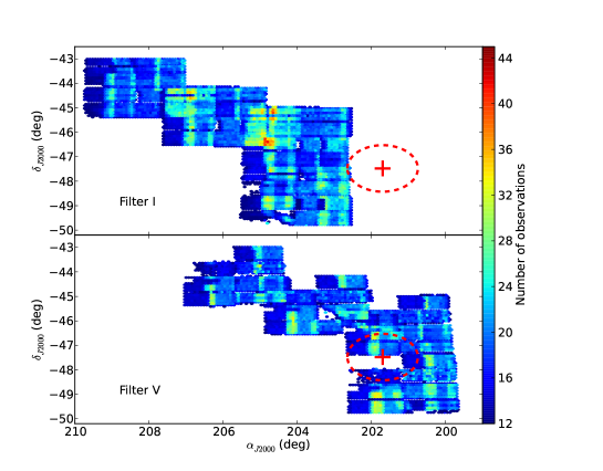
Figure 1: Density of observations around of $\omega$ Centauri in the V (bottom) and I (top) band: the color scale is proportional to the number of observations in each band. The large ’+’ symbol and dashed ellipse represent the center and tidal radius ($r_{t}=57$ arcmin) of the cluster, respectively.

All magnitudes were normalized to a reference catalog following the methodology used by Vivas et al. (2004). The normalization was performed independently in each CCD by using 500 to 1000 stars in each image. An ensemble clipped mean of the differences between magnitudes in each image and the reference image was calculated and added to all individual magnitudes in that image. The error added due to this zero point normalization was typically $<0.07$ mag.

Then, instrumental magnitudes in the reference images were calibrated using zero point corrections estimated by matching stars with two different catalogs: APASS (Henden et al. 2012), and DENIS (Epchtein et al. 1997), for stars observed in the V and I bands, respectively.

Saturation and limiting magnitudes in our catalog are respectively 11 and 19 mag in I, and 12.5 and 20 mag in V. Our final catalog has 456,539 stars.

$\omega$ Centauri is located at a galactic latitude of $b=14.97\textordmasculine$ (Harris 1996) which is low enough to expect large variations in extinction across the region. Dust maps from Schlegel et al. (1998), with the re-calibration proposed by Schlafly & Finkbeiner (2011), were used for correcting by interstellar extinction each individual star. The standard deviation of the interstellar extinction along all the region is $\sigma_{A_{V}}=0.07$ mag and $\sigma_{A_{I}}=0.04$ mag. A map of the color excess, E(B-V), over the survey region is shown in the Figure  2.

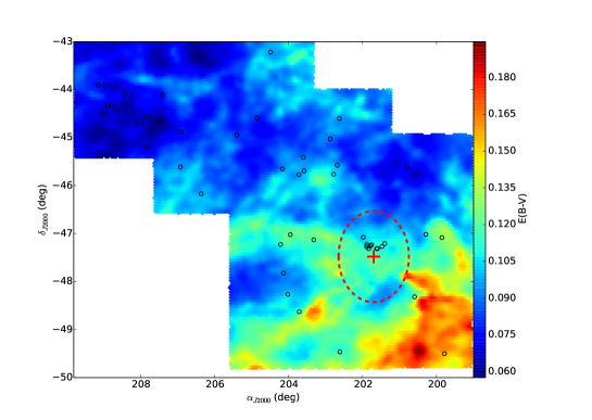
Figure 2: Reddening ($E{(B-V)}$) map around $\omega$ Centauri from Schlafly & Finkbeiner (2011). RR Lyrae stars detected in this work are represented by open circles. The center of the cluster and its tidal radius are represented by the red ’+’ symbol and dashed ellipse, respectively.

3 Search of RR Lyrae stars around $\omega$ Centauri

3.1 Selection of variable stars in the Color-Magnitude Diagram

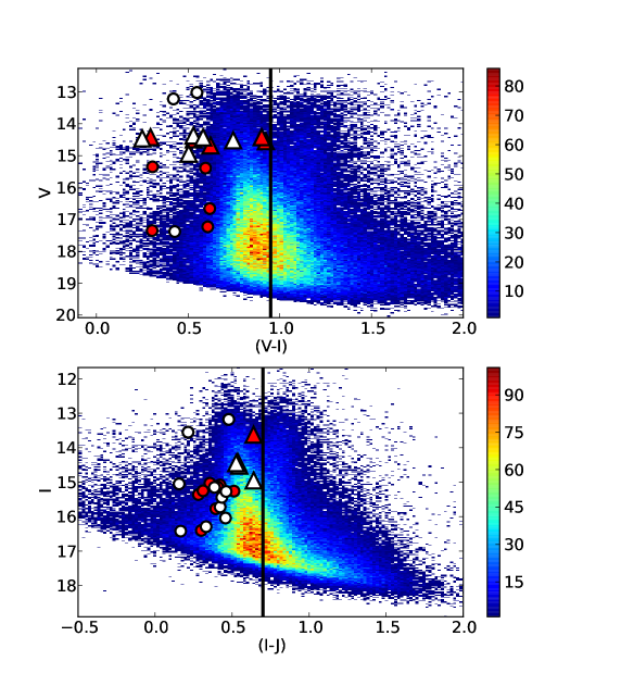
Figure 3: Hess diagrams for two different regions of the survey. The top panel shows a region which was observed in both V and I bands in our survey. The region shown in the bottom panel was observed only in I and we used 2MASS J-band to construct a color-magnitude diagram. Black vertical lines indicate the color cut for selecting RR Lyrae star candidates (however, the most interesting region was explored with no color cut). The triangle symbols indicate the confirmed RR Lyrae stars having a brightness similar to the Horizontal Branch of $\omega$ Centauri (see §4.2). Circles correspond to other RR Lyrae stars in the field of view (stars in the foreground or background of the cluster). RR Lyrae stars of the type $ab$ and $c$ are presented as red and white symbols, respectively. The color scale is proportional to the number of stars in each bin.

RR Lyrae stars are horizontal branch stars with spectral types A and F. A simple color cut would allow to significantly reduce the number of candidates to RR Lyrae stars. However, as explained in the last section not all of the survey area was observed in two photometric bands. To overcome this difficulty, we cross-matched our catalog with 2MASS (Skrutskie et al. 2006) to obtain either the $(V-J)$ or $(I-J)$ color in those regions observed in only one band. Magnitudes from 2MASS are single-epoch and RR Lyrae stars are expected to change color (change $T_{\rm eff}$) during the pulsation cycle. In addition, mean magnitudes may not be accurate if the lightcurves are poorly sampled. Thus, we searched for RR Lyrae stars with no color cut at all in the range of magnitudes of most interest for this work, $13.0<V<16.5$ (that is, around the magnitude of the horizontal branch of $\omega$ Cen). For the rest of the sample we applied the following color cut: $(V-I)\leq 0.95$ or $(I-J)\leq 0.70$ (Figure 3).

The next step toward identifying RR Lyraes was to detect variable stars in our time-series catalog. We calculated the Pearson distribution $\chi^{2}$ (Eq. 1) for all stars that passed our color cut and selected those ones whose probability is $P(\chi^{2})<0.01$, which corresponds to a 1% probability of the magnitude distribution being due to the observational errors:

$$\chi^{2}=\sum^{N}_{i=1}\frac{(m_{i}-\langle m\rangle)^{2}}{\nu\sigma^{2}_{i}}$$ (1)

where, $m_{i}$ …., $m_{N}$ are the individual magnitudes with observational errors $\sigma_{i}$, $\langle m\rangle$ is the mean magnitude, and $\nu=N-1$ is the degrees of freedom ($N$ is the number of observations by star).

Before calculating the $\chi^{2}$ probability we eliminated measurements that were potentially affected by cosmic rays or bad pixels by deleting any point whose magnitude was more than 4$\sigma$ away from the average magnitude of the star. This step helps to eliminate spurious variability.

3.2 Selection of RR Lyrae stars

Best possible periods in the range 0.2-1.2 days were determined for all variable candidates using the Lafler & Kinman (1965) algorithm (see also Vivas et al. 2004). Phased lightcurves were visually examined. RR Lyrae stars were finally identified based on their amplitude, period and the shape of the light curves. Forty-seven RR Lyrae stars (25 RRab and 23 RRc) were detected, 37 of which are new discoveries. Periods, amplitudes and ephemerids were refined by fitting templates of lightcurves of RR Lyrae stars to the data points, following the procedure described in Vivas et al. (2008). Lightcurves are shown in Figure 4.

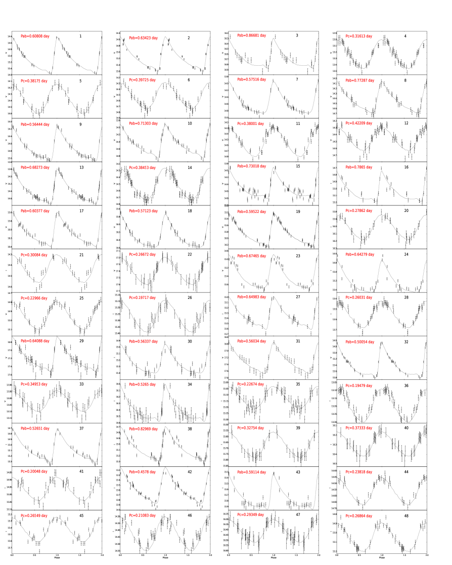
Figure 4: Light curves for RR Lyrae stars. Solid lines are the best template fitted to each light curve.

Distances were calculated by assuming the absolute magnitude relationships given by Catelan et al. (2004):

$$M_{I}=0.47-1.132logP+0.205logZ,\\$$ (2)

$$M_{V}=2.288+0.882logZ+0.108logZ^{2},\\$$ (3)

where

$$logZ=[Fe/H]+log(0.638\times 10^{[\alpha/Fe]}+0.362)-1.765,\\$$ (4)

Sollima et al. (2006) measured the metal abundance of 74 RR Lyrae stars in $\omega$ Cen, obtaining a mean value of [Fe/H]$=-1.7$ dex. On the other hand, following Del Principe et al. (2006), we adopted a value of $0.477$ for the $\alpha$-element abundance. Table 1 contains all the relevant information for the 48 RR Lyrae stars: column 1 indicates the star ID; columns 2 and 3 correspond to the right ascension and declination, respectively, whereas column 4 shows the number of times each star was observed. Columns 5-8 list the type of RR Lyrae star, our derived period and amplitude, and the heliocentric Julian day at maximum light. Columns 9 and 10 show the mean V and I magnitudes. The average E(B-V) in an area with 15 arcmin radius around each star are given in column 11. The heliocentric distance and the angular distance (in degrees) from the center of $\omega$ Centauri are shown in columns 12 and 13, respectively. Radial velocities for a sub-sample of the stars are reported in column 14. Finally, the ID number in the May 2014 version of the catalog of variable stars in globular clusters by Clement et al. (2001, C01) is given in column 15.

For several type c stars we found that one of 1-day aliases produced phased light curves as good as the one with the main period found for those stars. Based in our data there is no way to determine which one is the true period and which one is the spurious period. Table 1 contains double entries for the periods in those cases.

We estimated our completeness by producing a set of simulated light curves of RR Lyrae stars with the same temporal sampling and photometric errors as our data. The artificial light curves were then analyzed with the same tools we used for our data. At the typical magnitude range of RR Lyrae stars in $\omega$ Centauri, we were able to successfully recover the periods of type ab stars in $\gtrsim 90\%$ of the cases if the number of epochs (N) was larger than 20. The completeness drops to 85% for N=17 and 56% for N=12. The completeness of type c stars is lower; it is around 70% for the best sampled regions ($N>17$), dropping to 40% for N=12.

Table 1: RR Lyrae Stars

ID	$\alpha_{2000}$	$\delta_{2000}$	$N_{obs}$	Type	P	Amp	HJD	$\langle V\rangle$	$\langle I\rangle$	E(B-V)	$D$	$\theta$	RV	ID(C01)
	(deg)	(deg)			(day)	(mag)	(day)	(mag)	(mag)	mag	(kpc)	(deg)	(km s-1)
1	199.787506	-49.50225	22	ab	0.60808	1.15	2455706.66692	15.06$\pm$0.02	-	0.155	6.3 $\pm$1.0	2.4	114$\pm$19	-
2	199.855804	-47.08439	24	ab	0.63423	1.10	2455309.71655	15.11$\pm$0.02	-	0.130	6.6 $\pm$1.0	1.3	293$\pm$20	-
3	200.289261	-47.016312	17	ab	0.86681	0.58	2455309.73527	16.66$\pm$0.16	-	0.107	14.0 $\pm$3.0	1.1	-	-
4	200.595367	-48.31789	40	c	0.31613	0.46	2455324.63072	13.22$\pm$0.03	-	0.130	2.8 $\pm$0.4	1.1	-	175
5	200.793121	-45.59691	21	c	0.38175	0.46	2455597.8221	14.37$\pm$0.04	-	0.074	5.1 $\pm$0.8	2.0	123$\pm$ 10	-
6	201.40033	-47.20893	25	c	0.39725	0.46	2455324.68931	14.52$\pm$0.03	-	0.109	5.2 $\pm$0.8	0.3	-	160
7	201.473541	-47.2696	25	ab	0.57516	0.94	2455655.76307	14.49$\pm$0.03	-	0.111	5.1 $\pm$0.8	0.3	280$\pm$53	73
8	201.597946	-47.31337	25	ab	0.77287	0.63	2455655.76505	14.42$\pm$0.03	-	0.111	5.0 $\pm$0.8	0.2	-	54
9	201.619019	-47.31311	25	ab	0.56444	0.95	2455706.66799	14.68$\pm$0.03	-	0.111	5.6 $\pm$0.8	0.2	-	67
10	201.754318	-47.233349	25	ab	0.71303	0.95	2455596.91557	14.42$\pm$0.27	-	0.109	5.0 $\pm$1.3	0.2	-	7
11	201.792587	-47.258259	35	c	0.38001	0.52	2455706.69839	14.46$\pm$0.17	-	0.108	5.1 $\pm$1.1	0.2	-	36
12	201.832062	-47.313049	37	c	0.42209	0.35	2455597.79094	14.43$\pm$0.14	-	0.111	5.0 $\pm$1.0	0.2	-	75
13	201.886887	-47.22865	41	ab	0.68273	0.97	2455309.74263	14.33$\pm$0.03	-	0.106	4.8 $\pm$0.7	0.3	216$\pm$ 19	149
14	201.887589	-47.27296	41	c	0.38453	0.48	2455596.84259	14.50$\pm$0.03	-	0.109	5.2 $\pm$0.8	0.2	-	72
15	201.97934	-47.07737	38	ab	0.73018	0.91	2455597.88609	14.60$\pm$0.19	-	0.102	5.5 $\pm$1.2	0.4	-	172
16	202.612198	-49.46468	17	ab	0.7865	0.45	2455323.76461	-	15.03$\pm$0.03	0.114	9.6 $\pm$0.4	2.1	-	-
17	202.62558	-44.60067	25	ab	0.60377	0.80	2455309.68646	16.05$\pm$0.03	-	0.095	10.8 $\pm$1.6	3.0	-	-
18	202.68248	-45.576481	27	ab	0.57123	0.85	2455706.63748	16.26$\pm$0.04	-	0.097	11.8 $\pm$1.8	2.0	-	-
19	202.775803	-45.764069	41	ab	0.59522	1.04	2455321.75328	15.76$\pm$0.03	-	0.103	9.3 $\pm$1.4	2.0	-	-
20	202.869476	-45.028179	21	c	0.27862	0.34	2455596.85697	-	16.04$\pm$0.14	0.088	12.2 $\pm$1.1	2.6	-	-
21	203.317429	-47.12904	16	c	0.30084	0.26	2455655.75493	-	14.45$\pm$0.10	0.120	5.9 $\pm$0.4	1.2	-	-
22	203.579575	-45.693771	25	c	0.26672	0.41	2455323.70735	17.38$\pm$0.15	-	0.097	19.8 $\pm$4.1	2.2	-	-
23	203.595047	-45.412022	25	ab	0.67465	0.80	2455597.82386	15.39$\pm$0.02	-	0.092	8.0 $\pm$1.2	2.4	-	-
24	203.707916	-48.628139	21	ab	0.64279	0.72	2455309.67323	-	15.25$\pm$0.23	0.114	10.1 $\pm$1.3	1.8	-	-
25	203.715485	-45.770672	27	c	0.22966	0.31	2455706.68115	14.94$\pm$0.02	-	0.096	6.5 $\pm$0.9	2.2	-55$\pm$10	-
$26^{a}$	203.950912	-47.023251	21	c	0.19717	0.19	2455309.76025	-	15.27$\pm$0.08	0.122	7.8 $\pm$0.5	1.6	-	-
					0.24183
27	204.017181	-48.265869	19	ab	0.64983	0.63	2455324.68881	-	15.36$\pm$0.17	0.104	10.7 $\pm$1.1	1.7	-	-
28	204.134323	-47.82508	35	c	0.26031	0.26	2455321.70224	-	13.55$\pm$0.02	0.094	3.8 $\pm$0.1	1.7	-	-
29	204.164261	-45.651611	32	ab	0.64088	0.86	2455597.7796	17.23$\pm$0.23	-	0.091	18.6 $\pm$4.5	2.5	-	-
30	204.212128	-47.2262	25	ab	0.56337	0.45	2455309.69697	-	15.26$\pm$0.16	0.115	9.8 $\pm$1.0	1.7	-	-
31	204.482224	-43.218788	17	ab	0.56034	0.92	2455324.67663	17.35$\pm$0.29	-	0.097	19.5 $\pm$5.3	4.7	-	-
32	204.84198	-44.595249	24	ab	0.50054	1.16	2455596.91508	15.35$\pm$0.25	-	0.079	8.0 $\pm$2.0	3.6	-	-
33	205.394684	-44.94603	24	c	0.34953	0.16	2455655.74781	13.02$\pm$0.06	-	0.082	2.7 $\pm$0.4	3.6	-	-
34	206.357758	-46.170818	31	ab	0.5265	0.58	2455309.72722	-	16.40$\pm$0.15	0.097	16.6 $\pm$1.6	3.4	-	-
35	206.900879	-44.87455	40	c	0.22674	0.18	2455706.62415	-	15.15$\pm$0.07	0.078	7.8 $\pm$0.4	4.4	-	-
$36^{a}$	206.92006	-45.61159	37	c	0.19479	0.21	2455324.70204	-	13.18$\pm$0.07	0.094	3.0 $\pm$0.2	4.0	-	-
					0.24209
37	207.397919	-44.10767	21	ab	0.52651	0.60	2455323.71549	-	15.14$\pm$0.18	0.077	9.4 $\pm$1.0	5.2	-	-
38	207.469147	-44.640949	39	ab	0.82969	0.60	2455596.91604	-	15.08$\pm$0.19	0.059	10.3 $\pm$1.1	4.9	-	-
39	207.786301	-44.555771	21	c	0.32754	0.22	2455309.76984	-	15.72$\pm$0.08	0.066	11.1 $\pm$0.7	5.1	-	-
40	207.820847	-45.19574	23	c	0.37333	0.26	2455309.79996	-	16.29$\pm$0.10	0.068	14.9 $\pm$1.0	4.8	-	-
41	208.065308	-44.707298	22	c	0.20048	0.16	2455309.75057	-	14.95$\pm$0.06	0.066	7.0 $\pm$0.4	5.2	-	-
42	208.413483	-44.092201	36	ab	0.4578	0.73	2455655.76003	-	13.62$\pm$0.20	0.070	4.6 $\pm$0.5	5.8	-	-
43	208.628021	-44.437511	23	ab	0.59114	0.63	2455309.72658	-	15.77$\pm$0.18	0.066	13.0 $\pm$1.4	5.7	-	-
44	208.780243	-44.331718	24	c	0.23818	0.22	2455593.84126	-	14.52$\pm$0.08	0.069	6.0 $\pm$0.4	5.8	-	-
45	208.886917	-44.338421	23	c	0.26549	0.37	2455590.83373	-	15.44$\pm$0.15	0.069	9.3 $\pm$0.9	5.9	-	-
$46^{a}$	208.95462	-43.91272	36	c	0.21083	0.17	2455597.80525	-	14.41$\pm$0.07	0.072	5.5 $\pm$0.3	6.2	-	-
					0.26712
47	209.022217	-44.495121	34	c	0.29349	0.22	2455597.81265	-	16.42$\pm$0.08	0.068	15.0 $\pm$0.9	5.9	-	-
48	209.140732	-43.90432	30	c	0.26864	0.31	2455593.83375	-	15.05$\pm$0.12	0.077	7.8 $\pm$0.6	6.3	-	-

4 Properties of the RR Lyrae Stars

4.1 Previously known stars

Eleven out of the 48 RR Lyrae stars detected in our survey were already reported in the literature, all of them as members of $\omega$ Centauri (Clement et al. 2001). Ten of those stars are located between 10 and 25 arcmin from the center of $\omega$ Centauri; that is, well inside the tidal radius of the cluster (57 arcmin). There is no doubt these are cluster members which were recovered by our survey. The remaining star, #4 (or V175 in Clement et al. 2001), is in the outskirts of the cluster, at 66 arcmin from its center. The original source for this star goes back to Wilkens (1965) and no period or type of variable is reported. From our data, this star seems to be a real periodic star with a period of 0.316 d and a sinusoidal light curve. Although it resembles the properties of an RR Lyrae star of the type $c$, its mean magnitude is more than one magnitude brighter than the horizontal branch of the cluster. Bright variables such as Anomalous Cepheids and Population II Cepheids (BL Her) have been found in $\omega$ Cen (Kaluzny et al. 1997). However, those stars have periods ranging from 0.5 to 2.3d which are significantly larger than the period of V175. This seems to indicate that V175 is actually a foreground variable and not a real member of the cluster, although a measurement of the radial velocity would be needed to confirm it.

Our classification, periods and amplitudes for the 10 stars (6 of the type $ab$ and 4 of the type $c$) in the cluster agree quite well with the values reported in the list of variable stars in $\omega$ Centauri catalog (Clement et al. 2001, May 2014 version) The average of the absolute value of the differences between our periods and the published ones is only $8\times 10^{-4}$ days. Reassuringly, also the mean V magnitudes agree within 0.03 mags. These good agreements validate our methods for the photometry and detection of variables.

We found no new variables within the tidal radius of the cluster. On the other hand, we did not recover all known variables in the cluster but this is due to the fact that we intentionally left out of the survey most of the central part of the cluster. The reason is twofold: our objective is to study tidal debris around the cluster and then there is no special interest in the cluster itself, and, on the other hand, the resolution and median seeing of our data ($\sim$3 arcsec) is not adequate for crowded field photometry.

4.2 Distances and Spatial Distribution

The distance to $\omega$ Centauri based on the average of the 10 RR Lyrae stars inside its tidal radius is ($5.15\pm 0.23$) kpc. This value agrees very well with the distance of $5.4\pm 0.7$ derived by Weldrake et al. (2007) using (optical) observations of 69 RR Lyrae stars in the cluster, although it is somewhat short if compared with the value of $5.57\pm 0.08$ kpc recently derived by Navarrete (2015, in prep) from IR lightcurves of a similar number of RR Lyrae stars.

A histogram of the distribution of distances from the Sun for all the stars found in our survey can be seen in Figure 5. The histogram shows a pronounced peak at about $D=$ 5.2 kpc which naturally corresponds to the 10 cluster RR Lyrae stars discussed above. We used this diagram to select other stars around the cluster having a similar distance. Those stars may have been tidally disrupted from the cluster. The shaded region in the histogram encloses the region ($3.5\leq D\leq 9$ kpc) of our candidates for tidal debris. Within these limits we found 15 RR Lyrae stars outside the tidal radius of the cluster (that is, not counting the 10 cluster RR Lyrae stars).

Figure  6 shows the spatial distribution of the RR Lyrae stars detected in this work and the 25 stars within the distance limits above are marked with distinctive symbols. The distribution of those stars roughly along a line, as seen in this Figure, should not be immediately interpreted as a tidal tail since it is just a reflection of the shape of the survey?s footprint (see Figure 1). Anyway, there are candidate stars to debris up to $\gtrsim 6$ degrees from the center of the cluster.

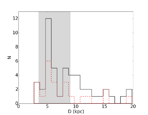
Figure 5: Distribution of distances of the RR Lyrae stars (solid line histogram). The distribution of the type-c RR Lyrae stars is shown with a red dashed histogram. The shaded region encloses the region of stars selected as candidates to tidal debris from the cluster.

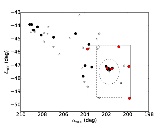
Figure 6: Spatial distribution of the RR Lyrae stars found in this survey. RR Lyrae stars in the range of distances of $\omega$ Centauri are indicated with either black or red dots. For the later we have measured radial velocities. Other RR Lyrae stars in the field (in either the foreground or background) are plotted with small star symbols. The black dashed circle corresponds to the tidal radius of $r_{t}=57$ arcmin of $\omega$ Centauri. The solid square and dashed rectangle show the regions explored by Leon et al. (2000) and Da Costa & Coleman (2008) respectively.

5 Analysis

In the last section we identified a group of 15 RR Lyrae stars that are located in the same distance range as $\omega$ Centauri and hence, are potentially tidal debris from the cluster. In this section we analyze this scenario from different perspectives.

5.1 Comparison with the properties of the cluster RR Lyrae stars

The sample of 15 candidates to debris is composed of 5 stars of the type $ab$ and 10 of the type $c$. It is somewhat surprising that the number of type c star candidates is larger than the number of type ab (a ratio of 2), since in general, type c stars are more rare. In $\omega$ Centauri itself there are 76 RR$ab$ and 59 RR$c$ (Clement et al. 2001), a ratio of 0.77. Thus, the sample of the candidates to cluster debris do not hold the same ratio. Miss-classification of the type c stars is a non-negligible possibility since, in the case of relatively few epochs in the light curves, eclipsing binaries of the type W UMa may mimic the shape of type $c$ RR Lyrae stars. The contamination due to this type of stars is higher at lower galactic latitude, like in this case, where the disk population is important (see Vivas et al. 2004; Mateu et al. 2009, for a complete discussion). High amplitude $\delta$ Scuti stars, which are also more common in the disk population, may have periods as long as type c stars and hence, they constitute an additional source of contamination. Hence, the true number of candidates to debris is likely lower than 15.

On the other hand, the mean period of the 5 type ab among the candidates to debris is 0.58 day. This is significantly different to the mean values of the periods of type ab stars found by Kaluzny et al. (2004, 86 stars, 0.656 days) and Weldrake et al. (2007, 40 stars, 0.647 days) in $\omega$ Centauri. The cluster has been given an Oosterhoff II classification. Figure 7 shows the distribution in the Bailey (period-amplitude) diagram for all debris candidates. For comparison, the diagram also contains the sample of RR Lyrae identified by Kaluzny et al. (1997) in $\omega$ Cen. For the RR Lyrae stars in this work having only I magnitude, we used the relationship ${\rm Amp}_{V}=0.075+1.497\times{}{\rm Amp}_{I}$ derived by Dorfi & Feuchtinger (1999). Out of the 5 type ab candidates to debris (red triangles in Figure 7), only 3 stars have periods $>0.6$ day and lie within the OoII population locus. The cluster RR Lyrae stars (star symbols) do show some dispersion in the Bailey’s diagram and thus, the distribution of our candidates is not inconsistent with the properties of the RR Lyrae stars in this diagram.

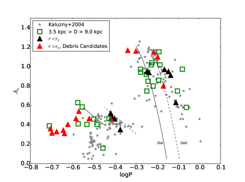
Figure 7: Distribution of the RR Lyrae stars in the range of distances from 3.5 to 9 kpc in the Bailey (period-amplitude) diagram. Stars within the tidal radius of the cluster are marked with black triangles while the ones outside the tidal radius (the candidates to debris) are indicated with red triangles. For reference, RR Lyrae stars in $\omega$ Centauri from Kaluzny et al. (2004) are shown with star symbols. Solid and dashed lines represent the typical locus of OoI and OoII clusters, respectively Cacciari et al. (2005).

5.2 Number of RR Lyrae stars expected in our survey

Does this group of 15 RR Lyrae stars constitute an overdensity of stars over the expected population of the halo/disk? In order to investigate this point, we calculated the expected number of RR Lyrae stars for the thick disc and halo over the survey area and in the range of distance of our debris candidates (3.5 kpc $<D<$9 kpc). For these calculations, we used the density profiles of type ab RR Lyrae stars in the Galactic thick disc and halo compiled in Table 4 in Mateu et al. (2009), which we reproduce here:

For the Halo, we used the Preston et al. (1991) model which has variable flattening density contours:

$$\rho_{halo}=\rho_{\odot}^{RR}\left(\frac{1}{R}\sqrt{x^{2}+y^{2}+\left(\frac{z}{c/a}\right)^{2}}\right)^{n}$$ (5)

where $(c/a)=0.5+(1-0.5(a/20))$ (a and c in kpc, Preston et al. 1991). The values for the slope and local density were taken from Vivas & Zinn (2006), are $n=-3.1\pm 0.1$ and $\rho_{\odot}^{RR}=4.2^{+0.5}_{-0.4}$ kpc^-3.

For the Thick Disk the number density is given by

$$\rho_{disc}=\rho_{\odot}^{RR}exp\left(-\frac{R_{gal}-R_{\odot}}{h_{R}}\right)exp\left(-\frac{\mid z\mid}{h_{z}}\right)$$ (6)

where $h_{R}=0.51$ kpc, $h_{z}=2.20$ kpc (Carollo et al. 2010). The local density of the thick disk ($\rho_{\odot}^{RR}=10$ kpc^-3) was taken from Layden (1995).

For the equations above we assumed the distance from the Sun to the galactic center as $R_{\odot}=8$ kpc (Reid 1993). The total number of RR Lyrae stars in each galactic component is given by integrating the above equations over the area of our survey and in the distance range of our candidates to debris:

$$N_{RRLS}^{halo}=\int_{3.5\mbox{ }kpc}^{9.0\mbox{ }kpc}\int_{b}\int_{l}\rho_{halo}(D,l,b)D^{2}\mbox{ }dD\mbox{ }cos(b)\mbox{ }db\mbox{ }dl$$ (7)

$$N_{RRLS}^{disc}=\int_{3.5\mbox{ }kpc}^{9.0\mbox{ }kpc}\int_{b}\int_{l}\rho_{disc}(D,l,b)D^{2}\mbox{ }dD\mbox{ }cos(b)\mbox{ }db\mbox{ }dl$$ (8)

Finally, the expected number of RR Lyrae stars ($ab$ type) in our survey area is:

$$N_{RRLS}^{survey}=N_{RRLS}^{halo}+N_{RRLS}^{disc}$$ (9)

Following the same method described in Mateu et al. (2009) to integrate those equations, we found $N_{RRLS}^{halo}=(14.2\pm 3.8)$ and $N_{RRLS}^{disc}=(3.7\pm 1.9)$, for a total of $N_{RRLS}^{survey}=(17.9\pm 4.2)$. If we assume a ratio $N_{ab+c}/N_{ab}=1.29$ (Layden 1995), there should be $(23.1\pm 4.8)$ RR Lyrae stars in the area of our survey. Taking into account the different completeness level of our survey (which depend on the number of epochs, see §3.2), we should expect ($22.2\pm 4.7$) RR Lyrae stars in the survey. The cited errors are Poisson statistics.

We also explored the expected number of RR Lyrae stars using the recent characterization of the thick disk and halo by Robin et al. (2014). These models predict $N_{RRLS}^{halo}=(18.5\pm 4.3)$ and $N_{RRLS}^{disc}=(4.9\pm 2.2)$ RR Lyrae stars (after completeness correction) depending on the thick disk model assumed (Eq. 1 and 2 in Robin et al. 2014), in agreement with the previous estimates.

It is clear that the expected number of RR Lyrae stars in the galactic components is of the same order (or even slightly higher) to what we actually found in our survey. Again, this does not favor the scenario of a significant amount of debris around the cluster since no overdensity of RR Lyrae stars has been observed.

5.3 Radial Velocities

Any recent debris from the cluster would be expected to have a similar radial velocity to that of the cluster. In order to investigate this issue we were able to obtain eight low resolution spectra of stars in our survey. Although the number is small, it can give us an idea if there is a preferential velocity among the candidates to debris.

The spectra was obtained with the R-C Spectrograph at the 1.5m Telescope operated by the SMARTS consortium at Cerro Tololo Interamerican Observatory (CTIO), Chile, and were reduced using standard IRAF routines. We obtained a signal to noise ratio $S/N>30$ with exposure times of 900s for each of the 8 observed stars (Figure 8). Some of the stars were observed at two different epochs (different nights). Although we took spectra of 8 stars, 2 of them, which were initially classified as type c, showed spectra that were too cool for this type of stars. Type c stars are in the bluest end of the instability strip region and hence have spectral types of A stars. The spectra of these 2 stars were late F/early G (see stars #49 and #50 in Figure 8). This finding supports our claim (§ 5.1) that the sample of type c stars may be contaminated by other types of variables. Coordinates and other data for these two stars are given in Table 2.

Table 2: Photometric Parameters for Stars #49 and #50

ID	$\alpha_{2000}$	$\delta_{2000}$	$N_{obs}$	P	Amp	$\langle V\rangle$	$\langle I\rangle$
	(deg)	(deg)		(day)	(mag)	(mag)	(mag)
49	202.643875	-45.994461	17	0.41530	0.25	14.02$\pm$0.04	-
50	206.151932	-44.192210	22	0.32759	0.19	-	14.18$\pm$0.02

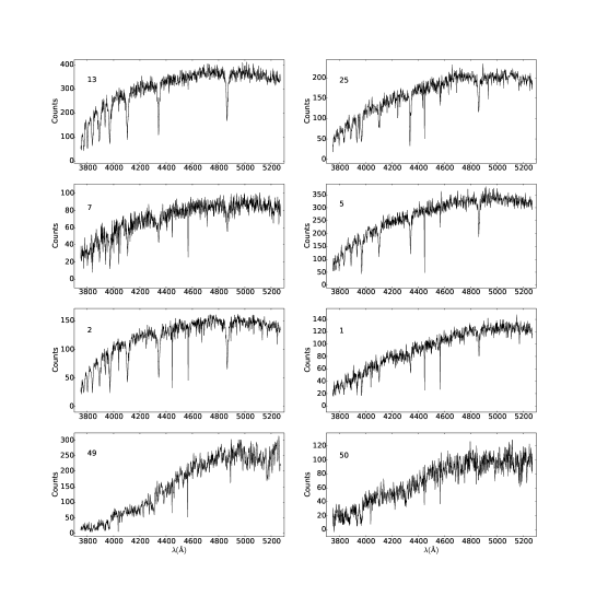
Figure 8: Spectra of the 8 variable stars observed with the SMARTS R-C spectrograph.

Radial velocities were then measured for 6 RR Lyrae stars via cross-correlation techniques using the IRAF routine $fxcor$. The templates for the correlation were five bright radial velocity standards from a list compiled originally by Layden (1994), which were observed with the same instrumental setup as the RR Lyrae stars. The correlation was carried out over the wavelength range $\lambda\lambda$3700-5300 Å, a spectral region that encompasses a number of strong features such as the Ca II K-line and H-line, and the H_δ, H_γ and H_β hydrogen lines. Heliocentric corrections were then applied to correct for the Earth’s motion. Systemic velocities were calculated by means of fitting a radial velocity curve template (see Vivas et al. 2008, for details). Figure  9 shows the templates used for obtaining the systemic velocities together with the radial velocities measured for each star. Typical errors for the radial velocities are of the order of 20 km/s. For star #7, the template of the radial velocity curve does not agree well with the data. We are quoting an error for this star which is the average difference between the observational points and the template.

In Figure 10 a histogram of the expected distribution of halo and thick disk stars in this part of the sky is plotted with a dashed and solid histogram, respectively. These distributions were obtained by extracting simulated data out of the Besan¸con Galaxy model (Robin et al. 2003) in this part of the sky (using a simple selection function of stars with $(V-I)\leq 0.95$ mag in colors and 14 mag $<V<16$ mag). The red histogram shows the location of the six RR Lyrae stars with radial velocity. Of those six objects, stars #7 and #13 are both located within the tidal radius. As expected they both have, within errors, similar radial velocity as the cluster (232.5 km/s, Dinescu et al. 1999). There are however no other stars that share the same velocity. Thus, radial velocities do not provide any indication for debris around the cluster. The RR Lyrae stars have velocities consistent with them belonging to the halo or thick disk population.

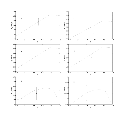
Figure 9: Two top rows: Radial velocity curve template of X Ari (dashed line) for RR Lyrae star $ab$-type. Bottom row: Radial velocity template T Sex and DH Peg (dashed line) for RR Lyrae star c-type (from Duffau et al. (2006, 2014)). The filled circles are the measured radial velocities.

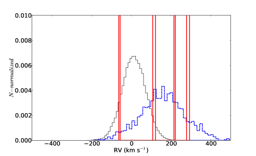
Figure 10: Radial velocity distributions of the halo (blue dashed histogram) and thick disk (black solid histogram) populations from the Besan¸con Galaxy Model (Robin et al. 2003) in the area of the sky covered by our survey. The red histogram correspond to the radial velocities of the six RR Lyrae stars for which we obtained spectroscopic observations.

5.4 Orbits

As a final test, we calculated the probability that each one of these 4 stars had a close encounter with the cluster sometime in the past. If that is the case, it may be argued that the stars were stripped off the cluster a long time ago. To do this, we calculated $10^{5}$ pairs of simulated orbits (for the cluster and each one of the RR Lyrae stars) using an axisymmetric Milky Way-like galactic model, following the one by Allen & Santillan (1991), scaled with the values $R_{0}=8.3$ kpc and $\Theta_{0}=239$ km s^-1 (see Brunthaler et al. 2011) and the methodology described in Pichardo et al. (2012). The axisymmetric background potential model consists of three components, a Miyamoto-Nagai spherical bulge and disk and a supermassive spherical halo. In addition to the position, distance and radial velocity given in Table 1, the orbit calculation requires proper motions. These were obtained from the UCAC4 catalog (Zacharias et al. 2013) and are given in Table  3. For $\omega$ Centauri itself, we used the proper motions measured by Dinescu et al. (1999): $\mu_{\alpha}=-5.08\pm 0.35$ mas; $\mu_{\delta}\cos(\delta)=-3.57\pm 0.34$ mas.

We calculated the probability of a close encounter between the cluster and the stars, which was defined as having a minimum approach $d_{min}\leq 100$ pc, or about the size of the tidal radius of the cluster. Orbits were integrated up to 1 Gyr in the past. We found low probabilities for such close encounters between the stars and the cluster. Even more, a closer examination of the circumstances of the few possible encounters casts doubts over the scenario of these stars to have been tidally stripped from the cluster. Figure 11 shows the details of the close encounters for the 4 stars investigated here. Each panel shows the distance of minimum approach ($d_{min}$) as a function of the relative velocity between the star and cluster ($V_{rel}$) at the moment of the encounter. In all 4 cases $V_{rel}$ peaks at $\sim 400$ km/s. That implies the stars have a much higher velocity than the escape velocity at the cluster center and at the cluster half-mass radius ($V_{0}=60.4$ km s^-1 and $V_{h}=44$ km s^-1, Gnedin et al. 2002). It is possible that a different mechanism such as ejection due to interaction with a binary system may be responsible for this discrepancy in the velocities (see for example Hut 1993; Pichardo et al. 2012). Anyway, the relevant point related to our work is that tidal stripping would not be an adequate mechanism to explain the current position and velocity of those stars.

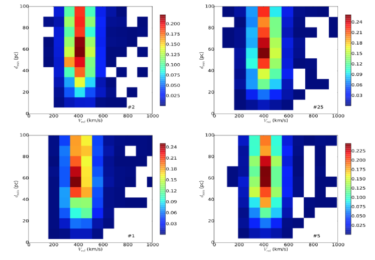
Figure 11: Distance of minimum approach ($d_{min}$) as a function of the relative star-cluster velocity for close encounters within 1 Gyr in the orbit simulations. The color code scales with the probability of a pair of orbits having such $d_{min}$ and $V_{rel}$.

Table 3: Input paramaters for the simulations.

ID	$\alpha_{2000}$	$\delta_{2000}$	$\mu_{\alpha}cos(\delta)$	$\mu_{\delta}$
	(deg)	(deg)	(mas/yr)	(mas/yr)
1	199.787506	-49.50225	8.5$\pm$2.8	-8.4$\pm$2.8
2	199.855804	-47.08439	-18.6$\pm$2.4	3.3$\pm$2.6
5	200.793121	-45.59691	-11.9$\pm$1.6	-0.6$\pm$1.6
25	203.715485	-45.77067	-11.1$\pm$2.9	6.8$\pm$2.9

6 CONCLUSIONS

We searched for tidal debris of the alleged progenitor galaxy of $\omega$ Centauri by using RR Lyrae stars as tracers of its population. We found 48 RR Lyrae variables (25 RR$ab$ and 23 RR$c$) in a region of $\sim 50$ deg². around the cluster.

Although several of those stars have a similar distance as the cluster, we conclude that there are no signs of stellar streams in the neighborhood of the globular cluster $\omega$ Centauri. This conclusion is based on the following:

• The expected number of RR Lyrae stars due to the halo and thick disk population of the Galaxy is consistent with the total number of RR Lyrae stars detected in this work. Thus, there is no overdensity of these stars in this region of the sky that can be linked to stellar debris.
  

• None of the radial velocities we obtained for stars outside the cluster had a radial velocity similar to that of the cluster. The caveat for this is that very few stars were measured spectroscopically. A firmer conclusion would necessarily need a more exhaustive spectroscopic study.
  

• The orbit simulations for the RR Lyrae stars in our survey with radial velocity show a very low probability that the stars were torn off the cluster in the past. The high relative velocity of the few possible close encounters suggests that the stars would have been ejected from the cluster by a different physical process other than tidal stripping.
  

• The ratio of between types $ab$ and $c$ among the stars at similar distance as the cluster is very different to the well known ratio of variables in the cluster. This suggests either it is a different stellar population and/or contamination for other type of stars is present in our survey.
  

This work confirms the results obtained by Da Costa & Coleman (2008), who also did not find a significant amount of tidal debris around the cluster. It is still puzzling that debris material have been found far away from the cluster (e.g. in the solar neighborhood) but not near the cluster itself. Our survey covers a large area of sky, but it is not uniform around the cluster in the sense that we preferentially surveyed along the path of the orbit of the cluster. We plan to pursue a larger and more uniform survey of RR Lyrae stars in the near future and include regions near the cluster not explored in this work.

References

- Allen & Santillan (1991) Allen, C. & Santillan, A. 1991, Rev. Mexicana Astron. Astrofis., 22, 255
- Anderson & van der Marel (2010) Anderson, J. & van der Marel, R. P. 2010, ApJ, 710, 1032
- Baltay et al. (2002) Baltay, C., Snyder, J. A., Andrews, P., et al. 2002, PASP, 114, 780
- Bedin et al. (2004) Bedin, L. R., Piotto, G., Anderson, J., et al. 2004, ApJ, 605, L125
- Bekki & Freeman (2003) Bekki, K. & Freeman, K. C. 2003, MNRAS, 346, L11
- Brunthaler et al. (2011) Brunthaler, A., Reid, M. J., Menten, K. M., et al. 2011, Astronomische Nachrichten, 332, 461
- Cacciari et al. (2005) Cacciari, C., Corwin, T. M., & Carney, B. W. 2005, AJ, 129, 267
- Cacciari et al. (2006) Cacciari, C., Sollima, A., & Ferraro, F. R. 2006, Mem. Soc. Astron. Italiana, 77, 245
- Carollo et al. (2010) Carollo, D., Beers, T. C., Chiba, M., et al. 2010, ApJ, 712, 692
- Carretta et al. (2010) Carretta, E., Bragaglia, A., Gratton, R. G., et al. 2010, ApJ, 714, L7
- Catelan et al. (2004) Catelan, M., Pritzl, B. J., & Smith, H. A. 2004, ApJS, 154, 633
- Clement et al. (2001) Clement, C. M., Muzzin, A., Dufton, Q., et al. 2001, AJ, 122, 2587
- Da Costa & Coleman (2008) Da Costa, G. S. & Coleman, M. G. 2008, AJ, 136, 506
- Del Principe et al. (2006) Del Principe, M., Piersimoni, A. M., Storm, J., et al. 2006, ApJ, 652,362
- Dinescu et al. (1999) Dinescu, D. I., Girard, T. M., & van Altena, W. F. 1999, AJ, 117, 1792
- Dorfi & Feuchtinger (1999) Dorfi, E. A. & Feuchtinger, M. U. 1999, A&A, 348, 815
- Drake et al. (2013) Drake, A. J., Catelan, M., Djorgovski, S. G., et al. 2013, ApJ, 763, 32
- Duffau et al. (2014) Duffau, S., Vivas, A. K., Zinn, R., Méndez, R. A., & Ruiz, M. T. 2014, A&A, 566, A118
- Duffau et al. (2006) Duffau, S., Zinn, R., Vivas, A. K., et al. 2006, ApJ, 636, L97
- Fernández Trincado et al. (2013) Fernández Trincado, J. G., Vivas, A. K., Mateu, C. E., & Zinn, R. 2013, Mem. Soc. Astron. Italiana, 84, 265
- Gnedin et al. (2002) Gnedin, O. Y., Zhao, H., Pringle, J. E., et al. 2002, ApJ, 568, L23
- Gratton et al. (2011) Gratton, R. G., Lucatello, S., Carretta, E., et al. 2011, A&A, 534, A123
- Harris (1996) Harris, W. E. 1996, AJ, 112, 1487
- Hilker et al. (2004) Hilker, M., Kayser, A., Richtler, T., & Willemsen, P. 2004, A&A, 422, L9
- Hut (1993) Hut, P. 1993, ApJ, 403, 256
- Ideta & Makino (2004) Ideta, M. & Makino, J. 2004, ApJ, 616, L107
- Jalali et al. (2012) Jalali, B., Baumgardt, H., Kissler-Patig, M., et al. 2012, A&A, 538, A19
- Kaluzny et al. (1997) Kaluzny, J., Kubiak, M., Szymanski, M., et al. 1997, A&AS, 122, 471
- Kaluzny et al. (2004) Kaluzny, J., Olech, A., Thompson, I. B., et al. 2004, A&A, 424, 1101
- King et al. (2012) King, I. R., Bedin, L. R., Cassisi, S., et al. 2012, AJ, 144, 5
- Lafler & Kinman (1965) Lafler, J. & Kinman, T. D. 1965, ApJS, 11, 216
- Law et al. (2003) Law, D. R., Majewski, S. R., Skrutskie, M. F., Carpenter, J. M., & Ayub, H. F. 2003, AJ, 126, 1871
- Layden (1994) Layden, A. C. 1994, AJ, 108, 1016
- Layden (1995) Layden, A. C. 1995, AJ, 110, 2288
- Leon et al. (2000) Leon, S., Meylan, G., & Combes, F. 2000, A&A, 359, 907
- Majewski et al. (2012) Majewski, S. R., Nidever, D. L., Smith, V. V., et al. 2012, ApJ, 747, L37
- Marino et al. (2012) Marino, A. F., Milone, A. P., Piotto, G., et al. 2012, ApJ, 746, 14
- Mateu et al. (2009) Mateu, C., Vivas, A. K., Zinn, R., Miller, L. R., & Abad, C. 2009, AJ, 137, 4412
- Merritt et al. (1997) Merritt, D., Meylan, G., & Mayor, M. 1997, AJ, 114, 1074
- Meylan (1987) Meylan, G. 1987, A&A, 184, 144
- Meylan et al. (1995) Meylan, G., Mayor, M., Duquennoy, A., & Dubath, P. 1995, A&A, 303, 761
- Miocchi (2010) Miocchi, P. 2010, A&A, 514, A52
- Mizutani et al. (2003) Mizutani, A., Chiba, M., & Sakamoto, T. 2003, ApJ, 589, L89
- Navarrete (2015) Navarrete, C. e. a. 2015, in preparation
- Noyola et al. (2010) Noyola, E., Gebhardt, K., Kissler-Patig, M., et al. 2010, ApJ, 719, L60
- Pichardo et al. (2012) Pichardo, B., Moreno, E., Allen, C., et al. 2012, AJ, 143, 73
- Preston et al. (1991) Preston, G. W., Shectman, S. A., & Beers, T. C. 1991, ApJ, 375, 121
- Reid (1993) Reid, M. J. 1993, ARA&A, 31, 345
- Robin et al. (2003) Robin, A. C., Reylé, C., Derrière, S., & Picaud, S. 2003, A&A, 409, 523
- Robin et al. (2014) Robin, A. C., Reylé, C., Fliri, J., et al. 2014, 1406.5384
- Schlafly & Finkbeiner (2011) Schlafly, E. F. & Finkbeiner, D. P. 2011, ApJ, 737, 103
- Schlegel et al. (1998) Schlegel, D. J., Finkbeiner, D. P., & Davis, M. 1998, ApJ, 500, 525
- Skrutskie et al. (2006) Skrutskie, M. F., Cutri, R. M., Stiening, R., et al. 2006, AJ, 131, 1163
- Sollima et al. (2006) Sollima, A., Borissova, J., Catelan, M., et al. 2006, ApJ, 640, L43
- Sollima et al. (2007) Sollima, A., Ferraro, F. R., Bellazzini, M., et al. 2007, ApJ, 654, 915
- Sollima et al. (2005) Sollima, A., Ferraro, F. R., Pancino, E., & Bellazzini, M. 2005, MNRAS, 357, 265
- Stock (1981) Stock, J. 1981, Rev. Mexicana Astron. Astrofis., 6, 115
- Trager et al. (1995) Trager, S. C., King, I. R., & Djorgovski, S. 1995, AJ, 109, 218
- Tsuchiya et al. (2004) Tsuchiya, T., Korchagin, V. I., & Dinescu, D. I. 2004, MNRAS, 350, 1141
- Vivas et al. (2008) Vivas, A. K., Jaffé, Y. L., Zinn, R., et al. 2008, AJ, 136, 1645
- Vivas & Zinn (2006) Vivas, A. K. & Zinn, R. 2006, AJ, 132, 714
- Vivas et al. (2004) Vivas, A. K., Zinn, R., Abad, C., et al. 2004, AJ, 127, 1158
- Watkins et al. (2009) Watkins, L. L., Evans, N. W., Belokurov, V., et al. 2009, MNRAS, 398, 1757
- Weldrake et al. (2007) Weldrake, D. T. F., Sackett, P. D., & Bridges, T. J. 2007, AJ, 133, 1447
- White & Shawl (1987) White, R. E. & Shawl, S. J. 1987, ApJ, 317, 246
- Wilkens (1965) Wilkens, H. 1965, Boletin de la Asociacion Argentina de Astronomia La Plata Argentina, 10, 66
- Wylie-de Boer et al. (2010) Wylie-de Boer, E., Freeman, K., & Williams, M. 2010, AJ, 139, 636
- Zacharias et al. (2013) Zacharias, N., Finch, C. T., Girard, T. M., et al. 2013, AJ, 145, 44