Acoustic (Ultrasonic) Non-Diffracting Beams: Some theory, and Proposals of Acoustic Antennas for several purposes ${}^{\>({\dagger})}$

Michel Zamboni-Rached^1,2  and  Erasmo Recami^2,3,4

¹ Photonics Group, Electrical & Computer Engineering, University of Toronto, CA

² DECOM, FEEC, Universidade Estadual de Campinas (UNICAMP), Campinas, SP, Brazil

${}^{3\;}$ Facoltà di Ingegneria, Università statale di Bergamo, Bergamo, Italy.

${}^{4\;}$ INFN—Sezione di Milano, Milan, Italy.

Abstract  –   On the basis of a suitable theoretical ground, we study and propose Antennas for the generation, in Acoustics, of Non-Diffracting Beams of ultrasound.  We consider for instance a frequency of about 40 kHz, and foresee fair results even for finite apertures endowed with reasonable diameters (e.g., of 1 m), having in mind various possible applications, including remote sensing.  We then discuss the production in lossy media of ultrasonic beams resisting both diffraction and attenuation.  Everything is afterward investigated for the cases in which high-power acoustic transducers are needed (for instance, for detection at a distance —or even explosion— of buried objects, like Mines).

[Keywords: Acoustic Non-Diffracting Beams; Truncated Beams of Ultrasound; Remote sensing; Diffraction, Attenuation, Annular transducers, Bessel beam superposition, High-power ultrasound emitters, Beams resisting diffraction and attenuation, Acoustic Frozen Waves, Detection of buried objects, Explosion of Mines at a distance].

1 Introduction

In this paper we aim at reporting about work performed by us during the last few years on theory and generation (in Acoustics) of Non-Diffracting Beams[1,2]of ultrasound; having in mind various possible applications, including remote sensing.  In the first part of this paper, we shall not deal, however, with the “(Acoustic) Frozen Waves”, confinig ourselves here to quote other articles, like Refs.[3,4], in which they have been investigated.

Acoustic Non-Diffracting Waves (ANDW) were first studied, generated, and applied by Lu et al., starting with 1992, for the particular, interesting case of the so-called (ultrasonic) X-shaped waves (see, e.g., Refs.[5,6]).  For reviews about Non-Diffracting Waves (NDW), including X-shaped waves (as well as Frozen Waves), one can see for instance Refs.[7,8] besides the initial Chapters in the already quoted [1,2].

The NDWs (including of course the ANDWs) arose interest because of their spatio-temporal localization, unidirectionality, soliton-like nature, and self-healing properties[1,2]: All of them bearing interesting consequences, from theoretical and experimental points of view, in all sectors of physics in which a role is played by a wave equation. The NDWs would keep such properties all along an infinite distance, only in the ideal case implying an infinite energy flux through any transverse plane. Such ideal NDWs cannot be practically generated, of course; and careful work was needed for finding out analytic expressions for realistic NDWs –for example truncated—, and then producing them (see Refs.[9,10] and refs. therein). Any realistic, finite-energy NDW will maintain its good properties only within its depth of field: much longer, however, than the one reached by a diffracting wave like the gaussian ones[1,2].

We are going to consider the problem of the truncated pulses in general (in electromagnetism, say), before passing to Acoustics.

1.1 Analytic Expressions for Truncated
Non-Diffracting Pulses

Let us go go on, therefore, to the problem of constructing in analytic form truncated Non-Diffracting Waves, in order to be able to produce them experimentally. We address here the case of pulses, since the case of beams have been extensively exploited elsewhere (see, e.g., Refs.[9,10] and refs. therein).

When one truncates an ideal non-diffracting pulse (INDP), the resulting wave field cannot be obtained, in general, in analytic form. One has to resort, instead, to the diffraction theory and perform numerical evaluations of the diffraction integrals, such as that, well known, of Rayleigh-Sommerfeld.  And, indeed, one can get important pieces of information about a truncated non-diffracting pulse (TNDP) by performing numerical simulations of its longitudinal evolution, especially when the pulse is axially symmetric.

However, let us mention first of all the possibility of obtaining truncated non-diffracting pulses in analytic form by a heuristic method. Subsequently, we are going to show how the solutions forwarded by our efficient method, expounded in Ref.[9] for beams, can be transformed into closed form expressions for truncated non-diffracting pulses[11].

1.2 A heuristic approach

First of all, let us recall that in Ref.[12] it was developed a preliminary method for describing the on-axis space-time evolution of truncated non-diffracting pulses, be they subluminal, luminal or superluminal.  Within that quite simple method, the on-axis evolution of a TNDP depends only on the frequency spectrum $S(\omega)$ of the corresponding INDP $\Psi_{{\rm INDP}}$; contrarily to the Rayleigh-Sommerfeld formula which depends on the explicit mathematical expression of $\Psi_{{\rm INDP}}$.  Such a heuristic method, due to its simplicity, can yield closed-form expressions which describe the on-axis evolution of innumerable TNDPs. In Ref.[12] one can find the analytic expressions for the truncated versions of several well-known localized pulses: subluminal, luminal, or superluminal. Therein, the theoretical results were compared with those obtained through the numerical evaluations of Rayleigh-Sommerfeld integrals, with excellent agreement. Here, we confine ourselves just to present an example of such noticeable agreements, by Figures 1 and 2.

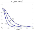
Figure 1: (Color online) Peak intensity evolution of a subluminal TNDP for three choices[12] of the parameters  [(1)  $V=0.995c\;$ and $\;b=1.5\times 10^{15}\;$Hz;  (2)  $V=0.998c\;$ and $\;b=6\times 10^{14}\;$Hz;  (3)  $V=0.9992c\;$ and $\;b=2.4\times 10^{14}\;$Hz]. In all cases the aperture radius is $R=4\;$mm.  Remember the linear relation $\omega=Vk_{z}+b$.  The continuous lines are obtained from the closed-form analytic expression (eq.23 in Ref.[12], while those represented by dotted lines come from the numerical simulation of the Rayleigh-Sommerfeld formula (eq.8 in [12]). The agreement is excellent: Practically, no difference is perceivable.

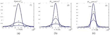
Figure 2: (Color online) On-axis evolution of the same subluminal TNDP considered in Fig.1, at three different instants of time [$t^{\prime}=0.11\;$ns, $t^{\prime\prime}=0.22\;$ns and $t^{\prime\prime\prime}=0.33\;$ns].  Figures a, b and c represent the cases (1),(2) and (3) respectively.  The continuous lines are the results obtained from the closed-form expression, while those represented by dotted lines come from the numerical simulation of the Rayleigh-Sommerfeld formula. Again, the agreement is excellent: No difference is detectable.

The mentioned approach in [12] is actually useful, because in general it furnishes closed-form analytic expressions avoiding the need of time-consuming numerical simulations; and also because those closed-form formulae provide an efficient tool for exploring several properties of the truncated localized pulses: as their depth of field, longitudinal pulse behavior, decaying rates, etc.

However, let us turn to a more rigorous approach.

1.3 Again on closed-forms for Non-Diffracting Pulses, in the Fresnel regime, generated by finite apertures

Let us fix our attention to the method developed in [9], that we shall call for brevity “the MRB method”; it can be found summarized, now, also in [13]. By that method, we got the analytic description of some monochromatic waves: namely, of a few (important) beams generated by finite apertures. The important point is that one can generalize the efficient method MRB, in the paraxial approximation, for the case of pulses.

Since we are going to use superpositions of Bessel-Gauss beams, let us start by recalling the form of the so-called Bessel-Gauss beam[14]:

$$\Psi_{\rm BG}(\rho,z)\;=\;-\frac{ikA}{2zQ}\,e^{ik(z+\frac{\rho^{2}}{2z})}\,J_{0}\left(\frac{ikk_{\rho}\rho}{2zQ}\right)e^{-\frac{1}{4Q}(k_{\rho}^{2}+\frac{k^{2}\rho^{2}}{z^{2}})}\ ,$$ (1)

which appears to be a Bessel beam transversally modulated by the Gaussian function.  Quantity $Q=q-ik/2z$, and $k_{\rho}$ (the transverse wavenumber associated with the modulated Bessel beam) is a constant.  [When $q=0$, the Bessel-Gauss beam results in the well-known Gaussian beam.  The Gaussian beam, and Bessel-Gauss’, Eq.(1), are among the few solutions to the Fresnel diffraction integral that can be obtained analytically].  The situation gets much more complicated, however, when facing beams truncated in space by finite circular apertures: For instance, a Gaussian beam, or a Bessel beam, or a Bessel-Gauss beam, truncated via an aperture with radius $R$. [In this case, the upper limit of the Fresnell integral becomes the aperture radius, and the analytic integration becomes very difficult, requiring recourse, as we were saying, to lengthy numerical calculations].  Afterward, let us also recall that –in the case of beams– we considered the solution given by the following superposition of Bessel-Gauss beams

$$\Psi(\rho,z)\;=\;-\frac{ik}{2\,z}\,\,e^{ik(z+\frac{\rho^{2}}{2\,z})}\displaystyle{\sum_{n=-N}^{N}}\,\frac{A_{n}}{Q_{n}}\,J_{0}\left(\frac{i\,k\,k_{\rho}\,\rho}{2\,z\,Q_{n}}\right)\,e^{-\frac{1}{4Q_{n}}(k_{\rho}^{2}+\frac{k^{2}\rho^{2}}{z^{2}})}\;,$$ (2)

quantities $A_{n}$ being constants, and $Q_{n}$ being given by  $Q_{n}=q_{n}-\frac{ik}{2z}$,  where the $q_{n}$ are constants that can assume complex values. In this superposition all beams possessed the same value of $k_{\rho}$.  In our previous work, we wanted the solution (2) to be able to represent beams truncated by circular apertures, in the case of Bessel beams, gaussian beams, Bessel-Gauss beams, and plane waves.  And, given one of such beams, truncated at $z=0$ by an aperture with radius $R$, we determined the coefficients $A_{n}$ and $q_{n}$ in such a way that Eq.(2) represented with fidelity the resulting beam. More details in the papers of ours quoted above.

Let us recall, before going on, that in previous work we found an equation which could be used for representing, on the plane $z=0$, truncated Gaussian, Bessel, Bessel-Gauss beams and truncated Plane waves; with the consequence that the evolution of such truncated beams was given by Eq.(2).  The interesting question, for us, is now: Is it possible to derive from what precedes also analytic descriptions of pulses truncated by finite apertures?: For instance, for TBP (truncated Bessel pulses), TBGP (truncated Bessel-Gauss pulses), TGP (truncated gaussian pulses), and TPP (truncated plane-wave pulses)? [even if we shall fix our attention only on truncated Bessel pulses].  We shall answer this question within the paraxial approximation; to this aim, consider an envelope $\psi(x,y,z;t)$ obeying the equation of the paraxial waves

$${{{\partial\psi}\over{\partial z}}+{1\over c}{{\partial\psi}\over{\partial t}}-{1\over{2k}}{\nabla_{\perp}}^{2}\psi\;=\;0}\;,$$ (3)

where the time dependence of $\psi$ is essential [and cannot be eliminated as in the case of beams]. When assuming axial symmetry, one can write:

$$\psi(\rho,z,t)\;=\;\int_{0}^{\infty}dk_{\rho}\;\int_{-\infty}^{\infty}du\,S(k_{\rho},u)\,J_{0}(k_{\rho}\rho)\;e^{i{u\over c}z}\;e^{-i{{k_{\rho}^{2}}\over{2k}}z}\;e^{-iut}\;,$$ (4)

where we replaced $\omega$ with the variable $u$ (since $\omega\equiv\omega_{0}$ will mean here the pulse central frequency).  As usual, it is  $k\equiv{\omega\over c}$,  and  $k_{z}\;=\;{u\over c}-{{k_{\rho}^{2}}\over{2k}}$.  If we know $\psi(\rho,z,t)$ on the plane $z=0$ of the aperture, it will be

$$\psi(\rho,0,t)\;=\;\int_{0}^{\infty}dk_{\rho}\,k_{\rho}\;\int_{-\infty}^{\infty}du\,S(k_{\rho},u)\,J_{0}(k_{\rho}\rho)\;e^{-iut}\;,$$ (5)

in terms of one Fourier-Bessel and one Fourier transformation.  By using the corresponding inverse transformations, one succeeds in writing the spectral function $S(k_{\rho},u)$ as a function of the field existing at the aperture!; namely:

$$S(k_{\rho},u)\;=\;{1\over{2\pi}}\;\int_{0}^{\infty}d\rho\,\rho\;\int_{-\infty}^{\infty}dt\,J_{0}(k_{\rho}\rho)\;e^{iut}\;\psi(\rho,0,t)\;.$$ (6)

Inserting Eq.(6) into Eq.(4), and reversing the order of the integrations over $k_{\rho}$ and $u$, one gets

$$\begin{array}[]{clr}&\psi(\rho,z,t)\;=\;\int_{0}^{\infty}d\rho^{\prime}\;\int_{-\infty}^{\infty}dt^{\prime}\\ \\ &\times\left\{\ \rho^{\prime}\psi(\rho^{\prime},0,t^{\prime})\left[\int_{0}^{\infty}dk_{\rho}k_{\rho}\,J_{0}(k_{\rho}\rho)\,J_{0}(k_{\rho}\rho^{\prime})\,e^{-i{{k_{\rho}^{2}}\over{2k}}z}\right]\ \left[\int_{-\infty}^{\infty}du\,e^{i{u\over c}(z-ct)}e^{iut^{\prime}}\right]\right\}\ .\end{array}$$ (7)

The last part in square brackets yields the Dirac delta  $2\pi\,\delta\left(t^{\prime}+{{z-ct}\over c}\right)$.  With some more algebra, one reaches the equation

$$\begin{array}[]{clr}&\psi(\rho,z,t)\;=\;\int_{0}^{\infty}d\rho^{\prime}\;\int_{-\infty}^{\infty}dt^{\prime}\ \{\rho^{\prime}\psi(\rho^{\prime},0,t^{\prime})\\ \\ &\times\left[-i{k\over z}\;\exp\left[i{{k\rho^{2}}\over{2z}}\right]\;\exp\left[i{{k{\rho^{\prime}}^{2}}\over{2z}}\right]\;J_{0}\left({{k\rho\rho^{\prime}}\over z}\right)\right]\ \left[2\pi\;\delta\left(t^{\prime}+{{z-ct}\over c}\right)\right]\ \}\ ,\end{array}$$ (8)

which can be finally integrated over $t^{\prime}$, without difficulties due to the presence of the delta, furnishing for a pulse the solution we were looking for:

$$\begin{array}[]{clr}\psi(\rho,z,t)&=\;\displaystyle{-i{k\over z}\;\exp\left[i{{k\rho^{2}}\over{2z}}\right]}\\ \\ &\times\displaystyle{\int_{0}^{\infty}d\rho^{\prime}\rho^{\prime}\;\psi\left(\rho^{\prime},0,-{{z-ct}\over c}\right)\;\displaystyle{e^{i{{k{\rho^{\prime}}^{2}}\over{2z}}}}\;J_{0}\left({{k\rho\rho^{\prime}}\over z}\right)}\ ,\end{array}$$ (9)

where one can notice that under the integral it now appears quantity $-(z-ct)/c$ instead of $t$.  Equation (9) is the analogous of the one found out by our MRB method for beams.

The integral solution (9) tells us that the pulsed field (envelope) can be obtained by merely knowing its value in the plane $z=0$ of the aperture, as a function of time and of the spatial coordinate.  The result in Eq.(9) is interesting also because it extends the MRB method to pulsed fields: In the sense that one can utilize any solution found by the said method[9] for beams, transforming it into a solution for pulses via a mere multiplication by the function $\exp[-(z-ct^{2})/(c^{2}T^{2})]$. More precisely:

—to get a truncated beam, it is enough to have at the aperture a field of the type  $\psi(\rho,0)\approx J_{0}(k_{\rho}\,\rho)\ {\rm sinc}(\rho/R)$;

—to get a truncated pulse, it will be enough to have at $z=0$ an analogous field of the type  $\psi(\rho,0)\approx J_{0}(k_{\rho}\,\rho)\,\exp(-t^{2}/T^{2})\ {\rm sinc}(\rho/R)$;

where the multiplying function  $\exp[-(z-ct^{2})/(c^{2}T^{2})]$  reduced to  $\exp(-t^{2}/T^{2})$  on supposing that $T>>2\pi/\omega$.  One can also notice that, having recourse to multiplying functions of the type  $\exp[-(t/T)^{2n}]$,  one can get a series of (for instance) step-shaped pulses.

2 Applications for acoustic (ultrasonic) non-diffracting pulses

Let us finally consider ultrasonic (acoustic) pulses, for instance with a central frequency of 40 kHz, generated by a finite aperture with radius $R=0.5$ m.  One may have in mind, for example, remote sensing, and the purpose of obtaining a realistic pulse which keeps its spot-size unvaried for, say, 20 m. We shall apply of course the results of our last subsection, which allow us to describe analytically several truncated pulses without any need, again, of lengthy numerical simulations.

Figure 3: (Color online) As an application of our last method to ultrasonic (acoustic) pulses, let us consider a truncated Bessel pulse with initial spot-radius of 15 cm, generated by a finite antenna with radius $R=0.5$ m. It is here neglected its attenuation (actually strong in the air when its central frequency is assumed to be 40 kHz). If one has in mind, for example, remote sensing, he may want our realistic pulse to keep its spot size unvaried for, say, 20 m.  The present set of figures, representing by colors the actual pulse evolution, does indeed show such a behavior.

Figure 4: This second set of figures shows, in terms of 3D plots, the evolutions of the same truncated Bessel pulse considered in the previous Figure.  In this case, the intensity is given by the height of $|\psi|^{2}$).   From these figures one can easily see the pulse spot (initially with a radius of 15 cm) to keep rather well its size for about 20 m, just with an oscillating intensity due to the edge-effects of the finite antenna.  Afterward, the pulse strongly deteriorates; and, to get better results by a Bessel pulse like this, one ought to use larger antennas.

Figure 5: (Color online) In this further figure we depict the evolution, during propagation, of the intensity peak of the same truncated Bessel pulse; still keeping no account of attenuation.

We shall confine ourselves, however, to just a few example. Let us start with a truncated Bessel pulse with spot-radius of 15 cm. For simplicity, we shall not take here into account the pulse attenuation, quite present for the said frequency in the air, even if one could take account of it without too much difficulty.

Such a Bessel pulse, a priori, can be easily generated. If we think in terms of a simple antenna, constituted by an array of annular transducers, then: (i) transducers do exist working with the mentioned frequency; (ii) amplitudes and phases of the vibrations are given as functions of the chosen pulse; (iii) the pulsed excitation (a modulation of the carrier wave) is the same for all transducers, and we choose precisely a temporal gaussian with $\Delta t=2.5\;$ms, hundred times larger than the period of the 40 kHz wave ($T=2.5x10^{-5}\;$ s). Incidentally, the choice of pulses with duration much longer than the carrier period is requested by the slow-envelope approximation, assumed by us when generalizing the MRB method for pulses.

Let us give an idea of the results by the help of suitable Figures.

The first set of figures, Fig.3, shows the pulse evolution by colors.  By contrast, the second set of figures, Fig.4, shows it in terms of 3D plots (the intensity being represented by te eigth of $|\psi|^{2}$).   From figures 4 one can clearly see the pulse spot (initially with a radius of 15 cm) to keep rather well its size for about 20 m, just with an oscillating intensity due to the edge-effects of the finite antenna. Afterward, the pulse strongly deteriorates; and, to get better results by such a Bessel pulse, one ought to use larger antennas.

By the the last figure, Fig.5, we depict the evolution of its intensity peak while propagating (still keeping no account of the attenuation).

2.1 Further Cases

Second case: Truncated Bessel beam with a spot radius of 23 cm

Suppose we want to get now a spot keeping its size for a larger distance, arriving at about thirty meters; while the ray of the generating antenna remains $R=0.5$ m.

As before, the pulse evolutions is first shown by colors (Fig.6), and then in terms of 3D plots (Fig.7), when the intensity is represented by the height of $|\psi|^{2}$.

One can see that the impulse spot radius (initially of 23 cm) maintains its value for about 30 m, oscillating in intensity due to the edge effects of the finite antenna.  Afterward, the pulse strongly deteriorates; once more, to get better results by a Bessel pulse like this, one ought to use larger antennas.

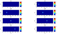
Figure 6: (Color online) As a second application of our method to ultrasonic (acoustic) pulses, let us consider now a truncated Bessel pulse with an initial spot-radius of 23 cm, generated by a finite antenna still with radius $R=0.5$ m. It is again neglected its attenuation (actually strong for a 40 kHz frequency). We wanted our realistic pulse to keep its spot size unvaried for the larger distance of about 30 m.  The present set of figures, representing by colors the actual pulse evolution, does indeed show such a behavior.

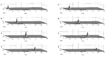
Figure 7: This second set of figures shows, in terms of 3D plots, the evolutions of the same truncated Bessel pulse considered in the previous Figure (its intensity being now the height of $|\psi|^{2}$). From the present figures one can see even better that the pulse spot (initially with a radius of 23 cm) keeps rather well its size for almost 30 m.  Afterward, the pulse strongly deteriorates; and, to get better results by a Bessel pulse like this, one has to use larger antennas.

By the the last figure, Fig.8, we depict the evolution of its intensity peak while propagating (when attenuation is neglected).

Figure 8: (Color online) In this further figure we depict the evolution, during propagation, of the intensity peak of the same truncated Bessel pulse.

Third case: Truncated Plane Wave Pulse

The first set of figures, Fig.9, shows the pulse evolution by colors; the second set, Fig.10, shows it by 3D plots (the pulse intensity being the height of $|psi|^{2}$).

In this case one clearly recognizes the interesting fact that the initial spot-radius, of 0.5 m, changes during propagation diminishing during the first 30 meters till 0.3 m.  After such a distance, however, the pulse starts to open: and its spot-size increases.

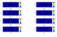
Figure 9: (Color online) As a third application of our method to ultrasonic (acoustic) pulses, let us now consider a Truncated Plane Wave Pulse, with initial spot-radius of 0.5 m.  It is interesting that the spot size does diminish during propagation, till a distance of 30 m. Only afterward, it start increasing, and the pulse opens.  The present set of figures shown such a behavior by colors.

Figure 10: This second set of figures shows, in terms of 3D plots, the evolutions of the Truncated Plane Wave Pulse considered in the previous Figure. From the present figures one can see even better that the pulse spot (initially with a radius of 0.5 m) reduces its size for almost 30 m, reaching the value of 0.3 m.  Only afterward the pulse opens (its spot-size increasing).

By the the last figure, Fig.11, we depict the evolution of its intensity peak while propagating (when attenuation is neglected).

Figure 11: (Color online) In this further figure we depict the evolution, during propagation, of the intensity peak of the same Plane Wave truncated pulse.

Fourth case: Pulse of Plane Wave Truncated and Focalized (at $z=20$ m)

The first set of figures, Fig.12, shows the pulse evolution by colors; the second set, Fig.13, shows it by 3D plots (the pulse intensity being the height of $|psi|^{2}$).

In this case one can clearly see that a focalization takes place at $z=20$ m.  This quite interesting result has been obtained by having recourse to a Plane Wave truncated (and pulsed) at the aperture, and modulated by a phase function similar to the transfer function of a convergent lens with a 20 m focal distance. The pulse leaves the antenna with a spot of 50 cm, which shrinks down (while the intensity increases), till reaching the distance of 20 m where the spot gets its minimum radius, of about 20 cm, and an intensity 20 times larger than the one at the aperture.

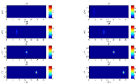
Figure 12: (Color online) As a third application of our method to ultrasonic (acoustic) pulses, let us now consider a Focalized Plane Wave (Truncated) Pulse, with initial spot-radius of 0.5 m.  In this case a focalization takes place at $z=20$ m. Such quite interesting result has been obtained by having recourse to a Plane Wave truncated (and pulsed) at the aperture, and modulated by a phase function similar to the transfer function of a convergent lens with a 20 m focal distance.  The present set of figures shown such a behavior by colors.

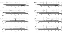
Figure 13: This second set of figures, in terms of 3D plots, shows the evolutions of the Focalized Plane Wave (Truncated) Pulse considered in the previous Figure. One can easily see that a focalization takes place at $z=20$ m.  This interesting result has been obtained —as we said– by having recourse to a Plane Wave truncated (and pulsed) at the aperture, and modulated by a phase function similar to the transfer function of a convergent lens with a 20 m focal distance.  The pulse leaves the antenna with a spot of 50 cm, which shrinks down (while the intensity increases), till reaching the distance of 20 m where the spot gets its minimum radius, of about 20 cm, and an intensity 20 times larger than the one at the aperture.

By the the last figure, Fig.14, we depict the evolution of its intensity peak while propagating (when attenuation is neglected).

Figure 14: (Color online) In this further figure we depict the evolution, during propagation, of the intensity peak of the same Focalized Plane Wave (Truncated) Pulse.

In the coming Section we are going to propose acoustic (ultrasound) antennas suitable for detection (or explosion) of buried objects, like mines.

See pages 1-23 of PARTEinWORD-ANTENNEIMPULSIACUSTICI.pdf