The dynamics of localized spot patterns for reaction-diffusion systems on the sphere

Abstract

In the singularly perturbed limit corresponding to a large diffusivity ratio between two components in a reaction-diffusion (RD) system, quasi-equilibrium spot patterns are often admitted, producing a solution that concentrates at a discrete set of points in the domain. In this paper, we derive and study the differential algebraic equation (DAE) that characterizes the slow dynamics for such spot patterns for the Brusselator RD model on the surface of a sphere. Asymptotic and numerical solutions are presented for the system governing the spot strengths, and we describe the complex bifurcation structure and demonstrate the occurrence of imperfection sensitivity due to higher order effects. Localized spot patterns can undergo a fast time instability and we derive the conditions for this phenomena, which depend on the spatial configuration of the spots and the parameters in the system. In the absence of these instabilities, our numerical solutions of the DAE system for $N=2$ to $N=8$ spots suggest a large basin of attraction to a small set of possible steady-state configurations. We discuss the connections between our results and the study of point vortices on the sphere, as well as the problem of determining a set of elliptic Fekete points, which correspond to globally minimizing the discrete logarithmic energy for $N$ points on the sphere.

,

1 Introduction

We analyze localized spot patterns for a two-component reaction-diffusion (RD) system on the surface of a sphere. In the singularly perturbed limit that corresponds to the large diffusivity ratio, such systems will often permit the formation of spatially localized spot patterns, These patterns are characterized by one or both solution components concentrating at certain points in the domain. At leading-order, the spot patterns are stationary, and in a companion paper by Rozada et al. [32], results for these quasi-equilibria structures were presented for the prototypical model of the Brusselator. Over long time scales, however, and for finite diffusivity ratios, the spots will indeed move on the sphere. The main goal of this paper is to derive and analyze these resultant slow spot dynamics.

We focus our analysis on the dimensionless Brusselator system given in terms of the activator $u=u(\bm{x},t)$ and the inhibitor $v=v(\bm{x},t)$ on the surface of the unit sphere, formulated as

$$\frac{\partial u}{\partial t}={\displaystyle\varepsilon}^{2}\operatorname{\Delta}_{S}u+F(u,v)\,,\qquad\tau\frac{\partial v}{\partial t}=\operatorname{\Delta}_{S}v+H(u,v)\,,$$ (1a)

where the nonlinear kinetics are defined by

$$F(u,v)\equiv{\displaystyle\varepsilon}^{2}\mathrm{E}-u+fu^{2}v\,,\qquad H(u,v)\equiv{\displaystyle\varepsilon}^{-2}\left(u-u^{2}v\right)\,,$$ (1b)

for constants $\mathrm{E}>0$, $\tau>0$, and $0<f<1$. In (1a), the surface Laplacian, $\operatorname{\Delta}_{S}$, is defined by

$$\operatorname{\Delta}_{S}\equiv\frac{1}{\sin^{2}\theta}\frac{\partial^{2}}{\partial\phi^{2}}+\frac{1}{\sin\theta}\frac{\partial}{\partial\theta}\left[\sin\theta\frac{\partial}{\partial\theta}\right]\,,$$ (2)

corresponding to the spherical coordinate system $\bm{x}=(x,y,z)=(\cos\phi\sin\theta,\sin\phi\sin\theta,\cos\theta)^{T}$, for longitudinal angular coordinate $\phi\in[0,2\pi)$ and latitudinal coordinate $\theta\in(0,\pi)$. The particular scaling of the non-dimensionalized system (1) has been primarily chosen so that the magnitude of the spot patterns for $u$ is $\mathcal{O}(1)$ in the limit ${\displaystyle\varepsilon}\to 0$. In A, we review the full details of the scalings leading to (1), as given in [32].

Figure 1: Full numerical solutions $u$ in (a) to (d), and $v$ in (e) to (h) of the RD system (1) computed using the closest-point method used in [32] with explicit Euler time integration. The parameter values are $f=0.8$, ${\displaystyle\varepsilon}=0.075$, $\tau=7.8125$, $\mathrm{E}=4$. Time steps were $\Delta t=0.005$ and $\Delta x=\Delta y=0.08$. Blue denotes small values, yellow middle values, and red large values. The top subplots display the patterns in the $(\phi,\theta)$ plane.

For small values of ${\displaystyle\varepsilon}$, localized spot patterns are readily observed in full numerical simulations of (1) when using random initial conditions close to the spatially uniform state $u_{e}={{\displaystyle\varepsilon}^{2}\mathrm{E}/(1-f)}$ and $v_{e}={(1-f)/(\mathrm{E}{\displaystyle\varepsilon}^{2})}$. For example, using one set of parameter values and with a $1\%$ random perturbation of the uniform state, Fig. 1 shows that the intricate transient dynamics at short times leads to the formation of six localized spots as time increases. Thus, given that spot-type patterns can emerge in the singularly perturbed limit, ${\displaystyle\varepsilon}\to 0$, it is of interest to asymptotically construct such patterns and then to analyze their stability and slow dynamics. A central question is to ask whether, beginning from an $N$-spot pattern, one can asymptotically derive from (1) a reduced dynamical system for the time evolution of the spot centers. From this limiting system, one can then determine the spatial locations of the centers of the spots that correspond to linearly stable steady-state patterns on the sphere.

1.1 Extending from the quasi-equilibrium study of Rozada et al. [32]

Our understanding of the quasi-static spot patterns on the sphere relies upon many results presented in the companion paper by Rozada et al. [32]. There, the method of matched asymptotic expansions was used in the limit ${\displaystyle\varepsilon}\to 0$ to construct the quasi-static $N$-spot solution for (1), with the spots centered at $\bm{x}_{1},\ldots,\bm{x}_{N}$ on the sphere. In the outer region, defined at ${\mathcal{O}}(1)$ distances from the spot locations, it was shown that the leading-order inhibitor concentration field, $v$, in (1) is given in terms of a sum of Green’s functions, where each spot is represented as a Coulomb singularity of the form $v\sim S_{j}\log|\bm{x}-\bm{x}_{j}|$ as $\bm{x}\to\bm{x}_{j}$, for $j=1,\ldots,N$. The spot strengths $S_{1},\ldots,S_{N}$ were found to satisfy a nonlinear algebraic system involving a Green’s matrix, representing interactions between the spots, and a nonlinear function arising from the local solution near an individual spot. An important parameter that is introduced was

$$\nu=\frac{1}{|\log{\displaystyle\varepsilon}|},$$ (3)

which arises during the matching process between the outer solutions, valid away from the spot centers, and the inner core solutions. This gauge function results from the logarithmic singularity of the Green’s function on the sphere.

Moreover, in the companion study, it was shown that from a numerical solution of a radially symmetric eigenvalue problem that if the spot strength exceeds some threshold, then the $j^{\textrm{th}}$ spot is linearly unstable to a non-radially symmetric peanut-shape perturbation near the spot. This linear instability was found to be the trigger of a nonlinear spot self-replication event, suggesting that this bifurcation is subcritical. In addition, a globally coupled eigenvalue problem (GCEP) was formulated that determines the stability properties of an $N$-spot pattern to locally radially symmetric perturbations near the spots. This GCEP was analyzed in [32] only for special spatial configurations $\{{\bm{x}_{1},\ldots,\bm{x}_{N}\}}$ of spots for which they have a common strength, i.e. $S_{c}=S_{j}$ for $j=1,\ldots,N$.

In this paper, we shall build upon the companion study [32] by presenting an asymptotic and numerical study of the slow spot patterns. We will also provide a more complete analysis of the quasi-equilibria patterns, particularly noting further distinguished limits as ${\displaystyle\varepsilon}\to 0$, and solutions with unequal spot strengths, which had not been previously uncovered in [32].

Our plan is as follows. First in §3, we shall derive the set of equations that governs the slow movement of the spot locations. We demonstrate that in the absence of any ${\mathcal{O}}(1)$ time-scale instability, the spots centers will slowly drift on an asymptotically long time-scale of order $\mathcal{O}({\displaystyle\varepsilon}^{-2})$. The governing equations take the form of differential algebraic equation (DAE) for the time-evolution of the spot locations, which depend on the current spot strengths. The main technical challenge in deriving this DAE is due to the higher-order matching between the inner (near-spot) and outer solutions. In particular, this asymptotic matching must account for inter-spot interactions, the slow dynamics of the patterns, and the correction terms that arise due to the projection the spherical geometry onto the local tangent plane approximation near the $j^{\textrm{th}}$ spot.

After having done so, we shall return in §4 to the study of the quasi-equilibrium solutions and provide a new analysis that accounts for the distinguished limits that arise when $E$ in (1) is either $\mathcal{O}(1)$ or simultaneously tends to zero when $\nu\to 0$. We identify a set of patterns of quasi-equilibrium patterns, not remarked in [32], that consists of spots of mixed strengths, and we demonstrate that such mixed patterns are all unstable on an $\mathcal{O}(1)$ time-scale. We furthermore extend the prior study by applying numerical path-following methods to the nonlinear algebraic system in order to illustrate the bifurcation structure. Notably, we demonstrate the new result that, in the regime $\mathrm{E}=\mathcal{O}(\sqrt{\nu})$, the bifurcation structure can exhibit imperfection sensitivity if a certain condition on the spot locations does not hold.

In §5, we perform numerical simulations of the DAE system in the parameter regime for which the quasi-equilibrium spot patterns are linearly stable. By beginning from random initial configurations for $N=2$ to $N=8$ spots, we identify the steady-state patterns having large basins of attraction. A particularly difficult configuration to identify is for $N=8$, where the stable steady-state pattern is a $45^{\circ}$ “twisted cuboid”: two parallel rings containing four equally-spaced spots, with the spots phase shifted by $45^{\circ}$ between each ring (see Fig. 10). In fact, this special 8-spot pattern is an elliptic Fekete point set. Our main results are summarized in §6, and we discuss numerous open problems for future study.

1.2 Connections and differences with other works

There is a wealth of literature on the formation of RD patterns in both simple and more complicated domains. Let us review how the work our this paper fits into the wider community.

For the situation where only one of the two solution components is localized, the spots are said to exhibit semi-strong interactions. In this semi-strong interaction limit, and in a 1-D spatial domain, there have been many studies of the dynamics of localized patterns for specific reaction-diffusion systems; this includes the Gierer-Meinhardt (GM) model [13, 34, 11], the Gray-Scott (GS) model [9, 10, 34, 7], the Schnakenberg model [31], a three-component RD system modeling gas-discharge [37], the Brusselator model [36], a model for hot-spots of urban crime [35], and a general class of RD models [24]. In these studies, a wealth of different analytical techniques have been used, including the method of matched asymptotic expansions, Lyapanov-Schmidt reductions, geometric singular perturbation theory, and the rigorous renormalization approach of [11]. In contrast, for the case of a 2-D domain, there are only a few studies of the dynamics of localized spot patterns by formal asymptotic analysis (see e.g. [17, 16, 6]), as the analytical techniques available in 2-D are, to a large extent, very different in nature to those for the simpler 1-D case.

There have been many numerical studies of RD patterns on the sphere and other compact manifolds (c.f. [5, 19, 1, 12, 20, 23, 38]), many of which are motivated by specific problems in biological pattern formation for both stationary and time-evolving surfaces (c.f. [27, 18, 29]). Most prior analytical studies of pattern formation on surfaces have been restricted to the sphere, and focus on analyzing the development of small amplitude spatial patterns that bifurcate from a spatially uniform steady-state at some critical parameter value. Near this bifurcation point, weakly nonlinear theory based on equivariant bifurcation theory and detailed group-theoretic properties of the spherical harmonics have been used to derive and analyze normal form amplitude equations characterizing the emergence of these small amplitude patterns (c.f. [4, 8, 21, 22, 28, 38]). However, due to the typical high degree of degeneracy of the eigenspace associated with spherical harmonics of large mode number, these normal form amplitude equations typically consist of a large coupled set of nonlinear ODEs. These ODEs have an intricate subcritical bifurcation structure, with weakly nonlinear patterns typically only becoming stable past a saddle-node bifurcation point. As a result, the preferred spatial pattern that emerges from an interaction of these modes is difficult to predict theoretically. Moreover, although equivariant bifurcation theory is able to readily predict the general form of the coupled set of amplitude equations, the problem of calculating the coefficients in these amplitude equations for specific RD systems is rather intricate in general (see [4] for the case of the Brusselator).

In this paper and its companion [32], we propose an alternative theoretical framework for analyzing RD patterns on the sphere. In contrast to a weakly nonlinear framework, our theoretical analysis is not based on an asymptotic closeness of parameters to a Turing bifurcation point. Instead, it relies on an assumed large diffusivity ratio between the two components in the system. In this singularly perturbed limit, the Brusselator allows for the existence of localized quasi-equilibrium spot-type patterns for a wide range of parameters.

Related work on characterizing slow spot dynamics in a 2-D planar domain was done previously for the Schnakenberg model [16] and the Gray-Scott model [6]. Our analysis of slow spot dynamics on the sphere is rather more complicated than that for the planar case since we must carefully examine certain correction terms generated by the curvature of the sphere.

We also note that an important motivation for this paper is to better understand the connections that exists between the study of spot patterns on the sphere in RD systems, with the apparently similar study of point vortex motion on the sphere in Eulerian fluid mechanics. For the latter problem, the positions of the point vortices are similarly governed by a reduced dynamical system. This system has been under intense study over the past three decades (see [3, 15, 25, 26, 2] and the references therein).

2 Two principal results for slow spot dynamics

In this section, we present our main results for the slow dynamics of a collection of localized spots for (1) on the surface of the unit sphere. The first result, as originally derived in [32], is an asymptotic result characterizing quasi-equilibrium solutions of (1) when ${\displaystyle\varepsilon}\ll 1$. The result is as follows:

Principal Result 1 (Quasi-Equilibria, (2.15) in [32]).

For ${\displaystyle\varepsilon}\to 0$, the leading order uniformly valid quasi-equilibrium solution to (1) is described by an outer solution, valid away from the spots, and inner core solutions near each of the $N$ spots centered at $\bm{x}=\bm{x}_{j}$ for $j=1,\ldots,N$. These solutions are

$$u_{\mathrm{unif}}\sim{\displaystyle\varepsilon}^{2}\mathrm{E}+\sum_{i=1}^{N}U_{i,0}\left(\frac{|\bm{x}-\bm{x}_{i}|}{{\displaystyle\varepsilon}}\right)\,,\qquad v_{\mathrm{unif}}\sim\sum_{i=1}^{N}S_{i}L_{i}(\bm{x})-4\pi R\mathrm{E}+\overline{v}\,,$$ (4)

where $L_{i}(\bm{x})\equiv\log|\bm{x}-\bm{x}_{i}|$, $R\equiv\frac{1}{4\pi}(\log 4-1)$, and $\overline{v}$ is a constant. The leading-order radially symmetric inner core solution, $U_{i,0}$, is defined on the tangent plane to the sphere near the spot at $\bm{x}=\bm{x}_{i}$, and is found by numerical computation of the BVP (18). In (4), the spot strengths, $S_{i}$ for $i=1,\ldots,N$, satisfy the nonlinear algebraic system

$$\mathcal{N}(\bm{S})\equiv\Bigl{[}\bm{\mathrm{I}}-\nu(\bm{\mathrm{I}}-{\mathcal{E}}_{0})\mathcal{G}\Bigr{]}\bm{S}+\nu(\bm{\mathrm{I}}-{\mathcal{E}}_{0})\bm{\chi}(\bm{S})-\frac{2\mathrm{E}}{N}\bm{e}=\bm{0}\,.$$ (5)

Here $\bm{\mathrm{I}}$ is $N\times N$ identity matrix, $({\mathcal{E}}_{0})_{ij}=\frac{1}{N}$, $(\bm{S})_{i}=S_{i}$, $(\bm{\chi}(\bm{S}))_{i}=\chi(S_{i})$, $(\mathcal{G})_{ij}=L_{i}(\bm{x}_{j})$ for $i\neq j$ and $(\mathcal{G})_{ii}=0$, $(\bm{e})_{i}=1$, and $\nu={-1/\log{\displaystyle\varepsilon}}$. The values of $\chi(S_{i})$ are found by numerically solving the leading-order inner system (18) (see Fig. 13). In terms of the spot strengths, the constant $\overline{v}$ in (4) is

$$\overline{v}=\frac{2\mathrm{E}}{\nu N}+4\pi R\mathrm{E}+\frac{1}{N}\left[\bm{e}^{T}\bm{\chi}-\bm{e}^{T}\mathcal{G}\bm{S}\right]\,.$$ (6)

For a fixed configuration of spot locations, the linear stability of such quasi-equilibrium solutions to ${\mathcal{O}}(1)$ time-scale instabilities was investigated in [32]. There, it was found that, depending on the range of $\mathrm{E}$, $\tau$, and $f$, such instabilities can lead to either spot self-replication events, a spot-annihilation phenomena, or temporal oscillations of a spot profile. These instabilities are discussed in detail in §4. For $\mathrm{E}={\mathcal{O}}(1)$, our analysis in §4 shows that, to leading order in $\nu$, spot-patterns for which $S_{j}={\mathcal{O}}(1)$, for all $j=1,\ldots,N$, are linearly stable on an ${\mathcal{O}}(1)$ time-scale provided that $S_{j}<\Sigma_{2}(f)$ for all $j=1,\ldots,N$, where $\Sigma_{2}$ is referred to as the spot self-replication threshold.

However, in those parameter range where these $\mathcal{O}(1)$ time-scale instabilities are absent, the main result of this paper is to show that the quasi-equilibrium solution of (4) characterizes the slow dynamics of a localized spot pattern for (1) on the longer time scales of $\mathcal{O}({\displaystyle\varepsilon}^{-2})$. On this long time-scale, the slow dynamics of the centers of a collection of $N$ spots is characterized as follows:

Principal Result 2 (Slow spot dynamics).

Let ${\displaystyle\varepsilon}\to 0$. Provided that there are no $\mathcal{O}(1)$ time-scale instabilities of the quasi-equilibrium spot pattern, the time-dependent spot locations, $\bm{x}_{j}=(\cos\phi_{j}\sin\theta_{j},\sin\phi_{j}\sin\theta_{j},\cos\theta_{j})^{T}$, vary on the slow time-scale $\sigma={\displaystyle\varepsilon}^{2}t$, and satisfy the differential algebraic system (DAE):

$$\frac{\mathrm{d}\theta_{j}}{\mathrm{d}\sigma}=-\frac{2}{\mathcal{A}_{j}}\alpha_{1}(\bm{x}_{j})\,,\qquad\sin\theta_{j}\frac{\mathrm{d}\phi_{j}}{\mathrm{d}\sigma}=-\frac{2}{\mathcal{A}_{j}}\alpha_{2}(\bm{x}_{j})\,,\qquad j=1,\ldots,N\,,$$ (7a)

where $${\mathcal{A}}_{j}={\mathcal{A}}(S_{j};f) S_{j}$$ is a nonlinear function of defined via an integral in (41) (see Fig. 2), and

$$\begin{pmatrix}\alpha_{1}(\bm{x}_{j})\\ \alpha_{2}(\bm{x}_{j})\end{pmatrix}\equiv\sum_{\begin{subarray}{c}i=1\\ i\neq j\end{subarray}}^{N}S_{i}\begin{pmatrix}\frac{\partial L_{i}(\bm{x})}{\partial\theta}\\ \frac{1}{\sin\theta_{j}}\frac{\partial L_{i}(\bm{x})}{\partial\phi}\end{pmatrix}\Biggr{\rvert}_{\phi=\phi_{j},\theta=\theta_{j}}\,.$$ (7b)

The spot strengths $$S_{j} j=1,\ldots,N$$, for , are coupled to the slow dynamics by (5).

It is convenient to express the slow dynamics of the spot locations in a more explicit form. To do so, we use the cosine law $|\bm{x}-\bm{x}_{i}|^{2}=2(1-\cos\gamma_{i})$ to write $L_{i}$ in terms of spherical coordinates as

$$L_{i}=\frac{1}{2}\log\left[1-\cos\gamma_{i}\right]+\frac{1}{2}\log{2}\,,\qquad\cos\gamma_{i}=\cos\theta\cos\theta_{i}+\sin\theta\sin\theta_{i}\cos(\phi-\phi_{i})\,,$$

where $\gamma_{i}=\gamma_{i}(\phi,\theta)$ is the angle between $\bm{x}$ and $\bm{x}_{i}$. By using this form for $L_{i}$, (7) becomes

$$\frac{\mathrm{d}\theta_{j}}{\mathrm{d}\sigma} =-\frac{1}{\mathcal{A}_{j}}\sum_{\begin{subarray}{c}i=1\\ i\neq j\end{subarray}}^{N}\left(\frac{S_{i}}{1-\cos\gamma_{ij}}\right)\Bigl{[}\sin\theta_{j}\cos\theta_{i}-\cos\theta_{j}\sin\theta_{i}\cos(\phi_{j}-\phi_{i})\Bigr{]}\,,$$ (8a)

$$\qquad\sin\theta_{j}\frac{\mathrm{d}\phi_{j}}{\mathrm{d}\sigma} =-\frac{1}{\mathcal{A}_{j}}\sum_{\begin{subarray}{c}i=1\\ i\neq j\end{subarray}}^{N}\left(\frac{S_{i}}{1-\cos\gamma_{ij}}\right)\Bigl{[}\sin\theta_{i}\sin(\phi_{j}-\phi_{i})\Bigr{]}\,,$$ (8b)

for $j=1,\ldots,N$, where $\gamma_{ij}\equiv\gamma_{i}(\phi_{j},\theta_{j})$ is the angle between $\bm{x}_{i}$ and $\bm{x}_{j}$.

As an alternative to (8), we can also write (7) in terms of cartesian coordinates. Writing ${\bm{x}}_{j}$ as a column vector, and letting $T$ denote transpose, we will show in §3 that (8) is equivalent to

$$\frac{\mathrm{d}\bm{x}_{j}}{\mathrm{d}\sigma}=\frac{2}{\mathcal{A}_{j}}\left(\bm{\mathrm{I}}-{\mathcal{Q}}_{j}\right)\sum_{\begin{subarray}{c}i=1\\ i\neq j\end{subarray}}^{N}\frac{S_{i}\bm{x}_{i}}{|\bm{x}_{i}-\bm{x}_{j}|^{2}}\,,\qquad{\mathcal{Q}}_{j}\equiv\bm{x}_{j}\bm{x}_{j}^{T}\,,\qquad j=1,\ldots,N\,.$$ (9)

3 Asymptotic derivation of the slow spot dynamics

Our aim in this section is to construct a localized quasi-equilibrium spot pattern solution for the system (1) in the limit ${\displaystyle\varepsilon}\to 0$. Such solutions consist of two parts. The first consists of an outer region, where the solution varies slowly according to

$$u_{\mathrm{out}}\sim{\displaystyle\varepsilon}^{2}\mathrm{E}\quad\text{and}\quad\operatorname{\Delta}_{S}v_{\mathrm{out}}\sim-{\displaystyle\varepsilon}^{-2}H(u_{\mathrm{out}},v_{\mathrm{out}})\sim-\mathrm{E}.$$ (10)

The second part of the solution consists of localized inner regions of spatial extent ${\mathcal{O}}({\displaystyle\varepsilon})$ near each of the spots centered at $\bm{x}=\bm{x}_{j}$, where $\bm{x}_{j}=(\cos\phi_{j}\sin\theta_{j},\sin\phi_{j}\sin\theta_{j},\cos\theta_{j})^{T}$, for $j=1,\ldots N$.

3.1 Plan of action

The asymptotic analysis presented below is necessarily detailed and technical, so let us first outline the three main steps of the procedure.

(Step 1) We first apply a dominant balance argument and argue that the centers of the spots will move slowly on a time scale $\sigma$ defined by $\sigma={\displaystyle\varepsilon}^{2}t$, so that $\bm{x}_{j}=\bm{x}_{j}(\sigma)$. In the inner region near the $j^{\textrm{th}}$ spot we introduce the local coordinates $\bm{s}=(s_{1},s_{2})^{T}$ defined by

$$s_{1}\equiv{\displaystyle\varepsilon}^{-1}\left[\theta-\theta_{j}(\sigma)\right]\,,\qquad s_{2}\equiv{\displaystyle\varepsilon}^{-1}\sin\theta_{j}\left[\phi-\phi_{j}(\sigma)\right]\,,\qquad\sigma={\displaystyle\varepsilon}^{2}t\,.$$ (11)

By re-scaling into the inner region, we develop the zeroth (leading) and first-order equations for the two inner solutions, $u_{\mathrm{in}}=U_{j}(\bm{s},\sigma)$ and $v_{\mathrm{in}}=V_{j}(\bm{s},\sigma)$ near the $j^{\text{th}}$ spot. The leading-order inner problem is precisely the same as in [32]. The first correction, however, is new, and is necessary in order to establish the dynamics.

(Step 2) We return to the outer region and develop a uniformly-valid outer solution which includes the logarithmic behaviour near the inner region (expressed as a sum of Green’s functions) and the unknown source strengths, $S_{j}$. Matching the inner and outer solutions at leading-order gives Principal Result 1, i.e. a nonlinear algebraic equation for $S_{j}$ for a known set of $\bm{x}_{j}$. Both Steps 1 and 2 are nearly the same as in [32]. The only difference is that the matching procedure of Step 2 requires derivation of higher-order terms that are used later.

(Step 3) The derivation of the governing equation for the spot locations now follows from matching the inner and outer solutions at first order, and applying a solvability condition. A key difficulty that confronts us in this step is that the higher-order matching between inner and outer solutions requires not only matching the inter-spot interactions and slow dynamics of the patterns, but also the corrections that arise due to the projection of the spherical geometry onto the local tangent plane approximation.

Before proceeding with these three steps, we first establish the following lemma that explains how the outer coordinate, $\bm{x}$, can be re-written in terms of the inner coordinate, $\bm{s}$. The proof is presented in C.1.

Lemma 1 (Tangent plane transformation).

Suppose that $\theta_{j}\in(0,\pi)$. Then, for $|{\bm{x}}-{\bm{x}}_{j}|={\mathcal{O}}({\displaystyle\varepsilon})$ and $|\bm{s}|={\mathcal{O}}(1)$, we have

$$\bm{x}-{\bm{x}}_{j}={\displaystyle\varepsilon}\bm{J}_{j}{\bm{s}}+{\mathcal{O}}({\displaystyle\varepsilon}^{2})\,,\qquad|{\bm{x}}-{\bm{x}}_{j}|\sim{\displaystyle\varepsilon}\rho+\frac{{\displaystyle\varepsilon}^{2}}{2\rho}s_{1}s_{2}^{2}\cot\theta_{j}\,,\qquad\rho\equiv\left(s_{1}^{2}+s_{2}^{2}\right)^{1/2}\,,$$ (12a)

where $$\bm{s}\equiv(s_{1},s_{2})^{T} \bm{J}_{j} 3\times 2$$ and is the matrix defined by

$$\bm{J}_{j}^{T}\equiv\begin{pmatrix}\cos\phi_{j}\cos\theta_{j}&\sin\phi_{j}\cos\theta_{j}&-\sin\theta_{j}\\ -\sin\phi_{j}&\cos\phi_{j}&0\\ \end{pmatrix}\,.$$ (12b)

3.2 (Step 1) Governing equations near the spots

We begin by re-scaling the governing equations near the $j^{\text{th}}$ spot and proceed to develop the first two orders. First, we write $u_{\mathrm{in}}=U_{j}(\bm{s},\sigma)$ and $v_{\mathrm{in}}=V_{j}(\bm{s},\sigma)$, and expand

$$U_{j}(\bm{s},\sigma)=\sum_{n=0}^{\infty}{\displaystyle\varepsilon}^{n}U_{jn}\,,\qquad V_{j}(\bm{s},\sigma)=\sum_{n=0}^{\infty}{\displaystyle\varepsilon}^{n}V_{jn}\,.$$ (13)

In addition, upon introducing (11) into (2) and the time derivative, we obtain for ${\displaystyle\varepsilon}\ll 1$ that

$$\operatorname{\Delta}_{S}=\frac{1}{{\displaystyle\varepsilon}^{2}}\operatorname{\Delta}_{(s_{1},s_{2})}+\frac{1}{{\displaystyle\varepsilon}}\mathfrak{N}_{1}+{\mathcal{O}}(1)\,,\qquad\frac{\partial}{\partial t}={\displaystyle\varepsilon}\mathfrak{T}_{1}+{\displaystyle\varepsilon}^{2}\frac{\partial}{\partial\sigma}\,,$$ (14a)

where we have defined the additional operators,

$$\nabla_{(s_{1},s_{2})}\equiv\left(\frac{\partial}{\partial s_{1}},\frac{\partial}{\partial s_{2}}\right)\,,\qquad\operatorname{\Delta}_{(s_{1},s_{2})}\equiv\frac{\partial^{2}}{\partial s_{1}^{2}}+\frac{\partial^{2}}{\partial s_{2}^{2}}\,,$$ (14b)

$$\mathfrak{N}_{1}\equiv\cot\theta_{j}\left(\frac{\partial}{\partial s_{1}}-2s_{1}\frac{\partial^{2}}{\partial s_{2}^{2}}\right)\,,\qquad\mathfrak{T}_{1}\equiv-\left(\dot{\theta}_{j},\dot{\phi}_{j}\sin\theta_{j}\right)\cdot\nabla_{(s_{1},s_{2})}\,.$$ (14c)

Here the overdot indicates derivatives with respect to $\sigma$, We substitute (13) and (14) into (1), and equate powers of ${\displaystyle\varepsilon}$ to obtain inner problems near $\bm{x}=\bm{x}_{j}$. To leading order, on $\bm{s}\in{\mathbb{R}}^{2}$ we obtain the same set of equations as presented in [32] [c.f. their (2.1)]:

$$\operatorname{\Delta}_{(s_{1},s_{2})}U_{j0}-U_{j0}+fU_{j0}^{2}V_{j0} =0\,,$$ (15a)

$$\operatorname{\Delta}_{(s_{1},s_{2})}V_{j0}+U_{j0}-U_{j0}^{2}V_{j0} =0\,.$$ (15b)

At next order, and labelling $\bm{U}_{j1}\equiv(U_{j1},V_{j1})^{T}$ and $\bm{U}_{j0}\equiv(U_{j0},V_{j0})^{T}$, we find on $\bm{s}\in{\mathbb{R}}^{2}$ that

$$\mathfrak{L}\bm{U}_{j1}\equiv\operatorname{\Delta}_{(s_{1},s_{2})}\bm{U}_{j1}+{\mathcal{M}}_{j}\bm{U}_{j1}=-\mathfrak{N}_{1}\bm{U}_{j0}+\begin{pmatrix}\mathfrak{T}_{1}U_{j0}\\ 0\\ \end{pmatrix}\,,\qquad{\mathcal{M}}_{j}\equiv\begin{pmatrix}-1+2fU_{j0}V_{j0}&fU_{j0}^{2}\\ 1-2U_{j0}V_{j0}&-U_{j0}^{2}\\ \end{pmatrix}\,.$$ (16)

Indeed, it is the above set of equations that will be used to establish the dynamics of the spots.

3.3 (Step 2) The leading-order inner problem and initial matching

We now move on to solve the leading-order inner problem (15) and perform the leading-order matching between inner and outer solutions. This procedure will lead to Principal Result 1.

First, we seek a radially symmetric solution to (15) with matching conditions,

$$U_{j0}\to 0\quad\text{and}\quad V_{j0}\sim S_{j}\log\rho\quad\text{as $\rho\to\infty$,}$$ (17)

where $\rho\equiv(s_{1}^{2}+s_{2}^{2})^{1/2}$ is the distance from the spot along the tangent plane, and $S_{j}$, referred to as the spot strength, is a parameter to be determined (cf. [32]). Note that since $u_{\mathrm{out}}={\mathcal{O}}({\displaystyle\varepsilon}^{2})$ in the outer region, the far-field behavior of $U_{j0}$ matches with the outer solution.

As such, in (15) we set $U_{j0}=U_{j0}(\rho)$ and $V_{j0}=V_{j0}(\rho)$. In terms of $\operatorname{\Delta}_{\rho}\equiv\partial_{\rho\rho}+\rho^{-1}\partial_{\rho}$, (15) reduces to the following BVP system on $0<\rho<\infty$:

$$\operatorname{\Delta}_{\rho}U_{j0}-U_{j0}+fU_{j0}^{2}V_{j0}=0\,,\qquad\operatorname{\Delta}_{\rho}V_{j0}+U_{j0}-U_{j0}^{2}V_{j0}=0\,,$$ (18a)

$$U_{j0}^{\prime}(0)=V_{j0}^{\prime}(0)=0\,,\quad U_{j0}\to 0\,,\quad V_{j0}\sim S_{j}\log\rho+\chi+o(1)\,\text{ as $\rho\to\infty$}.$$ (18b)

In general, the solution of the above problem must be computed numerically, and we have included in B additional details and figures for such computations. In particular, the far-field constant $\chi=\chi(S_{j};f)$, which is needed for the slow dynamics, must be computed numerically. Upon integrating (18a) for $V_{j0}$, we obtain the identity $S_{j}=\int_{0}^{\infty}(U_{j0}^{2}V_{j0}-U_{j0})\rho\,\mathrm{d}{\rho}$.

Next, we relate the outer solution for $v$, valid away from the spots, to the inner solution $V_{j0}$. We first use the leading-order uniformly valid solution for $u$, given by $u_{\mathrm{unif}}\sim{\displaystyle\varepsilon}^{2}\mathrm{E}+\sum_{i=1}^{N}U_{i0}$, to calculate $H(u,v)$, defined in (1), in the sense of distributions as

$${\displaystyle\varepsilon}^{-2}(u-u^{2}v)\sim\mathrm{E}+2\pi\sum_{i=1}^{N}\left[\int_{0}^{\infty}(U_{i0}-U_{i0}^{2}V_{i0})\rho\,\mathrm{d}{\rho}\right]\sim\mathrm{E}-2\pi\sum_{i=1}^{N}S_{i}\delta(\bm{x}-\bm{x}_{i})\,.$$ (19)

In this way, we obtain from (1) that the leading-order outer approximation for $v$ satisfies

$$\operatorname{\Delta}_{S}v=-\mathrm{E}+2\pi\sum_{i=1}^{N}S_{i}\delta(\bm{x}-\bm{x}_{i})\,,\quad\text{where}\quad\sum_{i=1}^{N}S_{i}=2\mathrm{E}\,.$$ (20)

The solution to (20), subject to smoothness conditions at the two poles, can be written in terms of the unique source-neutral Green’s function $G(\bm{x};\bm{x}_{i})$ defined by

$$\operatorname{\Delta}_{S}G=\frac{1}{4\pi}-\delta(\bm{x}-\bm{x}_{i})\,\quad\text{and}\quad\int_{\text{unit sphere}}G\,\mathrm{d}{x}=0\,.$$ (21)

The well-known solution to (21) is

$$G(\bm{x};\bm{x}_{i})=-\frac{1}{2\pi}L_{i}(\bm{x})+R\,,\qquad R=\frac{1}{4\pi}[\log 4-1]\,\qquad L_{i}(\bm{x})\equiv\log|\bm{x}-\bm{x}_{i}|\,.$$ (22)

Thus, in terms of $G$, the solution to (20) is given by

$$v=-2\pi\sum_{i=1}^{N}S_{i}G(\bm{x};\bm{x}_{i})+\overline{v}=\sum_{i=1}^{N}S_{i}L_{i}(\bm{x})-4\pi R\mathrm{E}+\overline{v}\,,$$ (23)

for some constant $\overline{v}$ to be determined below from matching to each inner solution $V_{j0}$.

To determine the spot strengths, $S_{j}$ for $j=1,\ldots,N$, and the unknown constant $\overline{v}$, we match the outer and inner solutions for $v$. We expand the outer solution in (23) as $\bm{x}\to\bm{x}_{j}$ to obtain

$$v\sim S_{j}\log|\bm{x}-\bm{x}_{j}|-4\pi R\mathrm{E}+\overline{v}+\sum_{\begin{subarray}{c}i=1\\ i\neq j\end{subarray}}^{N}S_{i}L_{ij}+\sum_{\begin{subarray}{c}i=1\\ i\neq j\end{subarray}}^{N}S_{i}\nabla_{\bm{x}}L_{i}\bigr{\rvert}_{\bm{x}=\bm{x}_{j}}\cdot(\bm{x}-\bm{x}_{j})+\cdots\,,$$

where $L_{ij}\equiv\log|\bm{x}_{i}-\bm{x}_{i}|$. Then, we use (12a) to write this expression in the inner variable $\bm{s}$ as

$$v\sim S_{j}\left[\log{\displaystyle\varepsilon}+\log\rho+\frac{{\displaystyle\varepsilon}}{2\rho^{2}}s_{1}s_{2}^{2}\cot\theta_{j}\right]-4\pi R\mathrm{E}+\overline{v}+\sum_{\begin{subarray}{c}i=1\\ i\neq j\end{subarray}}^{N}S_{i}L_{ij}+{\displaystyle\varepsilon}\sum_{\begin{subarray}{c}i=1\\ i\neq j\end{subarray}}^{N}S_{i}J_{j}^{T}\nabla_{\bm{x}}L_{i}\bigr{\rvert}_{\bm{x}=\bm{x}_{j}}\cdot\bm{s}\,,$$ (24)

where $\rho=(s_{1}^{2}+s_{2}^{2})^{1/2}$ and $\bm{J}_{j}$ is defined in (12b). In contrast, the far-field behavior of the $j^{\textrm{th}}$ inner solution is $V_{j}\sim S_{j}\log\rho+\chi(S_{j})+{\displaystyle\varepsilon}V_{j1}+\cdots$. To match the far-field behavior of this inner solution with (24), we require that

$$S_{j}\log{\displaystyle\varepsilon}-4\pi R\mathrm{E}+\overline{v}+\sum_{\begin{subarray}{c}i=1\\ i\neq j\end{subarray}}^{N}S_{i}L_{ij}=\chi(S_{j})\,,\qquad j=1,\ldots,N\,,$$ (25a)

$$V_{j1}\sim\frac{S_{j}}{2\rho^{2}}s_{1}s_{2}^{2}\cot\theta_{j}+\sum_{\begin{subarray}{c}i=1\\ i\neq j\end{subarray}}^{N}S_{i}J_{j}^{T}\nabla_{\bm{x}}L_{i}\bigr{\rvert}_{\bm{x}=\bm{x}_{j}}\cdot\bm{s}\,,\,\,\,\text{ as $|\bm{s}|\to\infty$}\,;\qquad j=1,\ldots,N\,.$$ (25b)

From (25a), and noting the constraint in (20), we obtain that $S_{j}$ for $j=1,\ldots,N$ and $\overline{v}$ satisfy the $N+1$ dimensional nonlinear algebraic system

$$S_{j}+\nu\chi(S_{j})-\nu\sum_{\begin{subarray}{c}i=1\\ i\neq j\end{subarray}}^{N}S_{i}L_{ij}=\overline{v}_{c}\,,\quad j=1\,,\ldots,N\,;\qquad\sum_{i=1}^{N}S_{i}=2\mathrm{E}\,,$$ (26a)

where $$\nu L_{ij} \overline{v}_{c}$$, , and are defined by

$$\nu\equiv{-1/\log{\displaystyle\varepsilon}}\,,\qquad L_{ij}=\log|\bm{x}_{i}-\bm{x}_{j}|\,,\qquad\overline{v}\equiv\frac{\overline{v}_{c}}{\nu}+4\pi R\mathrm{E}\,.$$ (26b)

By writing (26a) in matrix form, we then eliminate the constant $\overline{v}_{c}$ to derive that the spot strengths satisfy the nonlinear algebraic system in (5). In terms of the spot strengths, the constant $\overline{v}$ is given in (6). This completes the derivation of Principal Result 1.

Now before proceeding to the final step and deriving of the dynamical equations for the spots, let us draw the reader’s attention to the far-field behaviour of $V_{j1}$ in (25b). The work of this section that had led to Principal Result 1 is identical to that shown in [32], with the exception of the details surrounding this higher-order far-field behaviour.

3.4 (Step 3) The solvability condition and higher-order matching

To derive the result in Principal Result 2 for the slow spot dynamics, we must analyze the first-order inner problem (16) subject to the far-field condition (see (25b)) that

$$\bm{U}_{j1}\equiv\begin{pmatrix}U_{j1}\\ V_{j1}\\ \end{pmatrix}\sim\begin{pmatrix}0\\ \frac{S_{j}}{2\rho^{2}}s_{1}s_{2}^{2}\cot\theta_{j}+\sum_{\begin{subarray}{c}i=1\\ i\neq j\end{subarray}}^{N}S_{i}J_{j}^{T}\nabla_{\bm{x}}L_{i}\bigr{\rvert}_{\bm{x}=\bm{x}_{j}}\cdot\bm{s}\\ \end{pmatrix}\,,\qquad\mbox{as}\quad\rho=|\bm{s}|\to\infty\,.$$ (27)

Of the four inhomogeneous terms in (16) and (27), the forcing term $\mathfrak{N}_{1}\bm{U}_{j0}$ in (16) and the term $S_{j}s_{1}s_{2}^{2}\cot\theta_{j}/(2\rho^{2})$ in (27) correspond to corrections to the leading-order tangent plane approximation to the sphere at $\bm{x}=\bm{x}_{j}$. These correction terms are present even for the case of a single stationary spot solution. In contrast, the two remaining inhomogeneous terms in (16) and (27) result either from inter-spot interactions or from the time operator, $\mathfrak{T}_{1}$, applied to $U_{j0}$.

With this motivation, we seek a decomposition for $\bm{U}_{j1}$ into a “static” component, reflecting correction terms to the tangent plane approximation, and a “dynamic” component resulting from inter-spot interactions. This decomposition of the solution $\bm{U}_{j1}$ to (16) with (27) has the form

$$\bm{U}_{j1}\equiv\begin{pmatrix}U_{j1}\\ V_{j1}\end{pmatrix}=\bm{U}_{j1}^{\text{e}}+\bm{U}_{j1}^{\text{d}}\,,\qquad\bm{U}_{j1}^{\text{e}}\equiv\begin{pmatrix}U_{j1}^{\text{e}}\\ V_{j,1}^{\text{e}}\end{pmatrix}\,,\qquad\bm{U}_{j1}^{\text{d}}\equiv\begin{pmatrix}U_{j1}^{\text{d}}\\ V_{j,1}^{\text{d}}\end{pmatrix}\,,$$ (28)

where, in terms of the operator $\mathfrak{L}$ of (16), $\bm{U}_{j1}^{\text{e}}$ satisfies

$$\mathfrak{L}\bm{U}_{j1}^{\text{e}}=-\mathfrak{N}_{1}\bm{U}_{j0}\,,\quad\bm{s}\in{\mathbb{R}}^{2}\,;\qquad\bm{U}_{j1}^{\text{e}}\sim\begin{pmatrix}0\\ \frac{S_{j}}{2\rho^{2}}s_{1}s_{2}^{2}\cot\theta_{j}\end{pmatrix}\,,\quad\mbox{as}\quad|\bm{s}|\to\infty\,.$$ (29)

In contrast, the dynamic component $\bm{U}_{j1}^{\text{d}}$ is taken to satisfy

$$\mathfrak{L}\bm{U}_{j1}^{\text{d}}=\begin{pmatrix}\mathfrak{T}_{1}U_{j0}\\ 0\end{pmatrix}\,,\quad\bm{s}\in{\mathbb{R}}^{2}\,;\qquad\bm{U}_{j1}^{\text{d}}\sim\begin{pmatrix}0\\ \bm{\alpha}\cdot\bm{s}\end{pmatrix}\,,\quad\mbox{as}\quad|\bm{s}|\to\infty\,.$$ (30a)

Here $$\bm{\alpha}$$, identified from the second term in (27), is given by

$$\bm{\alpha}\equiv\sum_{\begin{subarray}{c}i=1\\ i\neq j\end{subarray}}^{N}S_{i}J_{j}^{T}\nabla_{\bm{x}}L_{i}\bigr{\rvert}_{\bm{x}=\bm{x}_{j}}=\sum_{\begin{subarray}{c}i=1\\ i\neq j\end{subarray}}^{N}S_{i}\begin{pmatrix}\frac{\partial L_{i}}{\partial\theta}\\ \frac{1}{\sin\theta_{j}}\frac{\partial L_{i}}{\partial\phi}\end{pmatrix}\Biggr{\rvert}_{\phi=\phi_{j},\theta=\theta_{j}}\,.$$ (30b)

Next, we show that a particular solution to (29) can be identified analytically. The proof is presented in C.2.

Lemma 2 (Static component of first-order inner solution).

Suppose that $U_{0}(\rho)$ and $V_{0}(\rho)$, with $\rho=(s_{1}^{2}+s_{2}^{2})^{1/2}$, are radially symmetric solutions to

$$\operatorname{\Delta}_{(s_{1},s_{2})}U+F(U,V)=0\,,\qquad\operatorname{\Delta}_{(s_{1},s_{2})}V+H(U,V)=0\,,\quad 0<\rho<\infty\,,$$ (31a)

$$U\to 0\,,\qquad V\sim S_{j}\log\rho+\chi+o(1)\,,\quad\mbox{as}\quad\rho\to\infty\,,$$ (31b)

where $\operatorname{\Delta}_{(s_{1},s_{2})}\equiv\partial_{s_{1}s_{1}}+\partial_{s_{2}s_{2}}$. Then, consider the linearized problem for $\bm{U}_{1}$ on $\bm{s}\in{\mathbb{R}}^{2}$ formulated as

$$\mathfrak{L}\bm{U}_{1}\equiv\operatorname{\Delta}_{(s_{1},s_{2})}\bm{U}_{1}+{\mathcal{M}}\bm{U}_{1}=-\cot\theta_{j}\left(\bm{U}_{0s_{1}}-2s_{1}\bm{U}_{0s_{2}s_{2}}\right)\,,$$ (32a)

$${\mathcal{M}}\equiv\begin{pmatrix}F_{U}&F_{V}\\ H_{U}&H_{V}\\ \end{pmatrix}\Biggr{\rvert}_{(U,V)=(U_{0},V_{0})},\hskip 45.00006pt\qquad\bm{U}_{1}\sim\begin{pmatrix}0\\ \frac{S_{j}}{2\rho^{2}}s_{1}s_{2}^{2}\cot\theta_{j}\end{pmatrix}\text{ as $|\bm{s}|\to\infty$}\,.$$ (32b)

Here $\bm{U}_{1}\equiv(U_{1},V_{1})^{T}$ and $\bm{U}_{0}\equiv(U_{0},V_{0})^{T}$, Then, a solution to (32) is

$$\bm{U}_{1}=-\frac{s_{2}^{2}}{2}\cot\theta_{j}\left(\partial_{s_{1}}\bm{U}_{0}\right)+\cot\theta_{j}s_{1}s_{2}\left(\partial_{s_{2}}\bm{U}_{0}\right)\,.$$ (33)

By applying this lemma to (29) we identify the static component as

$$\bm{U}_{j1}^{\text{e}}=-\frac{s_{2}^{2}}{2}\cot\theta_{j}\partial_{s_{1}}\bm{U}_{j0}+\cot\theta_{j}s_{1}s_{2}\partial_{s_{2}}\bm{U}_{j0}\,,$$ (34)

where $\bm{U}_{j0}=(U_{j0},V_{j0})^{T}$ satisfies (18). The key implication of this lemma is that the determination of $\bm{U}_{j1}^{\text{e}}$ is independent of the particular form of the reaction kinetics. As such, this lemma can be readily used for analyzing the dynamics of localized spot patterns for other RD systems.

The final step in the analysis of the slow dynamics is to impose a solvability condition on the dynamic component (30a) for $\bm{U}_{j1}^{\text{d}}$. Since $\mathfrak{L}\left(\partial_{s_{i}}\bm{U}_{0}\right)=0$ for $i=1,2$, the dimension of the nullspace of the adjoint $\mathfrak{L}^{\star}$ is two-dimensional. For the homogeneous adjoint problem

$$\mathfrak{L}^{\star}\bm{\Psi}\equiv\operatorname{\Delta}_{(s_{1},s_{2})}\bm{\Psi}+{\mathcal{M}}_{j}^{T}\bm{\Psi}=0\,,$$ (35)

we look for separable solutions of the form

$$\bm{\Psi}(\rho,\omega)=\bm{P}(\rho)T(\omega)\,,\qquad\bm{P}\equiv\begin{pmatrix}P_{1}(\rho)\\ P_{2}(\rho)\end{pmatrix}\,,\qquad\operatorname{\Delta}_{\rho}\equiv\partial_{\rho\rho}+\frac{1}{\rho}\partial_{\rho}\,,$$ (36)

for local polar coordinates $\bm{s}=(\rho\cos\omega,\rho\sin\omega)^{T}$ where $T(\omega)=\{{\cos\omega,\sin\omega\}}$. Thus, $\bm{P}$ satisfies

$$\operatorname{\Delta}_{\rho}\bm{P}-\frac{1}{\rho^{2}}\bm{P}+{\mathcal{M}}_{j}^{T}\bm{P}=0\,,$$ (37)

with $\bm{P}\to\bm{0}$ as $\rho\to\infty$. To determine the appropriate far-field behavior for $\bm{P}$, we observe that since $U_{j0}\to 0$ exponentially as $\rho\to\infty$, then ${\mathcal{M}}_{j}$ from (16) satisfies

$${\mathcal{M}}_{j}^{T}\to\begin{pmatrix}-1&1\\ 0&0\\ \end{pmatrix}\,,\quad\text{ as $\rho\to\infty$}\,.$$

As such, the solution $P_{2}$ to (37) satisfies $P_{2}={\mathcal{O}}(\rho^{-1})$ as $\rho\to\infty$, consistent with the decaying solution to $\operatorname{\Delta}_{\rho}P_{2}-\rho^{-2}P_{2}=0$. We normalize the eigenfunction by imposing that $P_{2}\sim{1/\rho}$ as $\rho\to\infty$. With this normalization, and from the limiting form of the first row of ${\mathcal{M}}_{j}^{T}$ for $\rho\gg 1$, we conclude from (37) that $P_{1}\sim{1/\rho}$ as $\rho\to\infty$. In this way, we solve (37) subject to $\bm{P}\sim({1/\rho},{1/\rho})^{T}$ as $\rho\to\infty$.

We now impose a solvability condition on the solution to (30a) with $\bm{\Psi}_{1}=\bm{P}T(\omega)$. We let $B_{\sigma}\equiv\{{\bm{s}:\lvert\bm{s}\rvert\leq\sigma\}}$. By applying Green’s second identity to $\bm{U}_{j1}^{\text{d}}$ and $\bm{\Psi}_{1}$ we obtain

$$\lim_{\sigma\to\infty}\int_{B_{\sigma}}\left[\bm{\Psi}_{1}^{T}\mathfrak{L}\bm{U}_{j1}^{\text{d}}-(\bm{U}_{j1}^{\text{d}})^{T}\mathfrak{L}^{\star}\bm{\Psi}_{1}\right]\,d{\bm{s}}=\lim_{\sigma\to\infty}\int_{0}^{2\pi}\left(\bm{\Psi}_{1}^{T}\partial_{\rho}\bm{U}_{j1}^{\text{d}}-(\bm{U}_{j1}^{\text{d}})^{T}\partial_{\rho}\bm{\Psi}_{1}^{T}\right)\biggr{\rvert}_{\rho=\sigma}\sigma\,\mathrm{d}{\omega}\,.$$ (38)

We now use the limiting far-field asymptotic behavior

$$\bm{U}_{j1}^{\text{d}}\sim\begin{pmatrix}0\\ \alpha_{1}\rho\cos\omega+\alpha_{2}\rho\sin\omega\\ \end{pmatrix}\,,\qquad\bm{\Psi}_{1}\sim\begin{pmatrix}{1/\rho}\\ {1/\rho}\\ \end{pmatrix}T(\omega)\,,\quad\text{ as $\rho\to\infty$}\,,$$

to calculate the right hand-side of (38), labeled by $\Lambda$, as

$$\Lambda\equiv\int_{0}^{2\pi}\left[2\alpha_{1}\cos\omega+2\alpha_{2}\sin\omega\right]T(\omega)\,\mathrm{d}{\omega}=\begin{cases}2\pi\alpha_{1}&\text{ if $T(\omega)=\cos\omega$}\\ 2\pi\alpha_{2}&\text{ if $T(\omega)=\sin\omega$}\end{cases}\,.$$ (39)

Then, by substituting the right hand-side of (30a) into the left hand-side of (38), and using $\partial_{s_{1}}U_{j0}=U_{j0}^{\prime}(\rho)\cos\omega$ and $\partial_{s_{2}}U_{j0}=U_{j0}^{\prime}(\rho)\sin\omega$, we obtain that

$$\Lambda=-\lim_{\sigma\to\infty}\int_{0}^{\infty}\int_{0}^{2\pi}P_{1}(\rho)\left[\theta_{j}^{\prime}U_{j0}^{\prime}(\rho)\cos\omega+\sin\theta_{j}\phi_{j}^{\prime}U_{j0}^{\prime}(\rho)\sin\omega\right]\rho T(\omega)\,\mathrm{d}{\rho}\,\mathrm{d}{\sigma}\,.$$ (40)

Upon using the two forms $T(\omega)=\cos\omega$ and $T(\omega)=\sin\omega$, (40) with (39) for $\Lambda$, reduces to (7a), where we have defined ${\mathcal{A}}_{j}={\mathcal{A}}(S_{j};f)$ by

$$\mathcal{A}_{j}\equiv\int_{0}^{\infty}U_{j0}^{\prime}(\rho)P_{1}(\rho)\rho\,\mathrm{d}{\rho}\,,$$ (41)

which appears in the ODE part of our result (7) for slow spot dynamics. Then, by substituting the second expression for $\bm{\alpha}=(\alpha_{1},\alpha_{2})^{T}$, as given in (30b), into (7a) we obtain the slow dynamics (7) as written in Principal Result 2.

To implement (7), we must numerically compute ${\mathcal{A}}(S_{j};f)$ from first solving the core problem (18) for $U_{j0}$ and then the adjoint problem (37) with far-field behavior $\bm{P}\sim({1\rho},{1/\rho})^{T}$ as $\rho\to\infty$. For $f=0.3$, in the left panel of Fig. 2 we plot ${\mathcal{A}}_{j}$ versus $S_{j}$ for $f=0.3$. In the right panel of Fig. 2 we plot ${\mathcal{A}}_{j}$ versus $S_{j}$ for $f=0.4$, $f=0.5$, $f=0.6$, and $f=0.7$.

Figure 2: Left: ${\mathcal{A}}_{j}$ versus $S_{j}$ for $f=0.3$. Right: ${\mathcal{A}}_{j}$ versus $S_{j}$ for $f=0.4$, $f=0.5$, $f=0.6$, and $f=0.7$, as shown. The thin vertical lines in these figures is the spot self-replication threshold $S_{j}=\Sigma_{2}(f)$ (see (44)). For $S_{j}>\Sigma_{2}(f)$, the quasi-equilibrium spot solution is linearly unstable on an ${\mathcal{O}}(1)$ time-scale. On the range $0<S_{j}<\Sigma_{2}(f)$ we observe that ${\mathcal{A}}_{j}<0$. In this figure, the values of $f$ decrease in the direction of the arrow.

Finally, we show how (9) follows from (7). We first differentiate $\bm{x}$ with respect to $\sigma$ to derive $\bm{x}_{j}^{\prime}=\bm{J}_{j}\left(\theta_{j}^{\prime},\phi_{j}^{\prime}\sin\theta_{j}\right)^{T}$, where $\bm{J}_{j}$ is defined in (12b). In (7a) we then use the first expression in (30b) for $\bm{\alpha}$ and pre-multiply both sides of the resulting expression with $\bm{x}_{j}^{\prime}$. This yields that

$$\bm{x}_{j}^{\prime}=-\frac{2}{{\mathcal{A}}_{j}}\bm{J}_{j}\bm{J}_{j}^{T}\sum_{\begin{subarray}{c}i=1\\ i\neq j\end{subarray}}^{N}S_{i}\nabla_{\bm{x}}L_{i}\bigr{\rvert}_{\bm{x}=\bm{x}_{j}}\,.$$

A direct calculation using (12b) shows that $\bm{J}_{j}\bm{J}_{j}^{T}=\bm{\mathrm{I}}-{\mathcal{Q}}_{j}$, where ${\mathcal{Q}}_{j}=\bm{x}_{j}\bm{x}_{j}^{T}$. In addition, we have $\nabla_{\bm{x}}L_{i}\bigr{\rvert}_{\bm{x}=\bm{x}_{j}}={(\bm{x}_{j}-\bm{x}_{i})/|\bm{x}_{j}-\bm{x}_{i}|^{2}}$. In this way, we get

$$\bm{x}_{j}^{\prime}=-\frac{2}{{\mathcal{A}}_{j}}\left[\bm{\mathrm{I}}-{\mathcal{Q}}_{j}\right]\sum_{\begin{subarray}{c}i=1\\ i\neq j\end{subarray}}^{N}S_{i}\frac{(\bm{x}_{j}-\bm{x}_{i})}{|\bm{x}_{j}-\bm{x}_{i}|^{2}}\,.$$ (42)

We then multiply both sides of this expression by $\bm{x}_{j}^{T}$ to obtain

$$\frac{1}{2}\frac{\mathrm{d}|\bm{x}_{j}|^{2}}{\mathrm{d}\sigma}=\left(1-|{\bm{x}}_{j}|^{2}\right)C_{j}\,,\quad C_{j}\equiv-\frac{2}{{\mathcal{A}}_{j}}\sum_{\begin{subarray}{c}i=1\\ i\neq j\end{subarray}}^{N}\frac{S_{i}}{|\bm{x}_{j}-\bm{x}_{i}|^{2}}\left(|{\bm{x}}_{j}|^{2}-|{\bm{x}}_{j}||{\bm{x}}_{i}|\cos\gamma_{ij}\right)\,,$$ (43)

where $\gamma_{ij}$ is the angle between $\bm{x}_{i}$ and $\bm{x}_{j}$. If $|\bm{x}_{j}(0)|=1$ for $j=1,\ldots,N$ and $\bm{x}_{i}(0)\neq\bm{x}_{j}(0)$ for $i\neq j$, then one solution to (43) is $|\bm{x}_{j}(\sigma)|=1$ for all $\sigma\geq 0$, so that, as expected, the centers of the spots remain on the unit sphere for all time. Along this specific solution $C_{j}\neq 0$ since $S_{i}>0$ for $i=1,\ldots,N$. Finally, (9) follows from (42) by noting that $\left(\bm{\mathrm{I}}-{\mathcal{Q}}_{j}\right)\bm{x}_{j}=0$ when $\bm{x}_{j}^{T}\bm{x}_{j}=1$.

4 Quasi-equilibrium spot patterns: existence and stability

As we characterized in Principal Result 2, quasi-equilibrium spot patterns will exhibit slow spot dynamics on a long ${\mathcal{O}}(\epsilon^{-2})$ time-scale. However, as was shown in [32], such patterns can be unstable on an ${\mathcal{O}}(1)$ time-scale in certain parameter regimes. In order to analyze the stability of the quasi-equilibrium spot patterns, we must first analyze the bifurcation behavior of the solution set of the nonlinear algebraic system (5) for the spot strengths $S_{1},\ldots,S_{N}$ for a given spatial configuration $\{{\bm{x}_{1},\ldots,\bm{x}_{N}\}}$ of spots. The stability analysis in [32] focused largely on quasi-equilibrium spatial patterns for which the spots have a common spot strength. Our goal here is to extend this prior analysis by identifying solutions to (5) where the spots can have rather different spot strengths. The stability of these patterns is analyzed through an extension of the stability analysis of [32]. Our analysis below will consider the two asymptotic ranges $\mathrm{E}=\mathcal{O}(1)$ and $\mathrm{E}=\mathcal{O}(\nu^{1/2})$, where different behavior occurs. Before considering these ranges of $\mathrm{E}$, we first outline the stability analysis of [32].

4.1 Stability criterion for the quasi-equilibrium spot patterns

The stability analysis in [32] allowed for perturbations of the quasi-equilibrium spot pattern that are either radially symmetric or non-radially symmetric in an ${\mathcal{O}}(\epsilon)$ neighborhood of each spot.

The linear stability of the quasi-equilibrium pattern with respect to non-radially symmetric perturbations near each spot was studied in §3.1 of [32] from the numerical computation of an eigenvalue problem. There, it was found that a spot centered at $\bm{x}_{j}$ is unstable to a peanut-shape perturbation when $S_{j}>\Sigma_{2}(f)$. The subscript on $\Sigma$ refers to instability with respect to the local peanut-splitting angular mode $\cos{2\omega}$ where $\omega=\arg(\bm{x}-\bm{x}_{j})$ as $\bm{x}\to\bm{x}_{j}$. The curve $\Sigma_{2}$ versus $f$ is plotted in Fig. 4 of [32], and we have

$$\Sigma_{2}(0.3)\approx 11.89\,,\quad\Sigma_{2}(0.4)\approx 8.21\,,\quad\Sigma_{2}(0.5)\approx 5.96\,,\quad\Sigma_{2}(0.6)\approx 4.41\,,\quad\Sigma_{2}(0.7)\approx 3.23\,.$$ (44)

This peanut-shaped unstable mode was found numerically in [32] to trigger, on an ${\mathcal{O}}(1)$ time-scale, a nonlinear spot self-replication event for the $j^{\textrm{th}}$ spot when $S_{j}>\Sigma_{2}(f)$.

In contrast to the non-radially symmetric case, the stability analysis of the quasi-equilibrium spot pattern with respect to radially symmetric perturbations near each spot is more intricate since this analysis is based on properties of a globally coupled eigenvalue problem (GCEP) (cf. [32]). To formulate the stability problem, we first linearize (1) around the quasi-equilibrium solution $u_{\textrm{qe}}$ and $v_{\textrm{qe}}$ by introducing $\psi$ and $N$ by

$$u=u_{\textrm{qe}}+e^{\lambda t}\psi\,,\qquad v=v_{\textrm{qe}}+e^{\lambda t}N\,.$$

The spectral problem for $\psi$ and $N$ is singularly perturbed, with an inner region near each spot and an outer region away from the spot locations. We now summarize the singular perturbation analysis of §3.2–3.4 of [32], for the formulation of the GCEP.

In terms of the core solution $V_{j0}$ and $U_{j0}$, the inner problem near the $j^{\textrm{th}}$ spot is to determine the radially symmetric solution to

$$\operatorname{\Delta}_{\rho}\psi_{j}-\psi_{j}+2fU_{j0}V_{j0}\psi_{j}+fU_{j0}^{2}N_{j}=\lambda\psi_{j}\,,\qquad\operatorname{\Delta}_{\rho}N_{j}+\psi_{j}-2U_{j0}V_{j0}\psi_{j}-U_{j}^{2}N_{j}=0\,,$$ (45a)

subject to the boundary conditions

$${\psi}_{j}^{\prime}(0)={N}_{j}^{\prime}(0)=0\,;\qquad\psi_{j}\to 0\,,\quad{N}_{j}\sim\log\rho+B_{j}+o(1),\text{ as $\rho\to\infty$}\,,$$ (45b)

for $\psi_{j}(\rho)$, $N_{j}(\rho)$ on $0<\rho<\infty$, where $\operatorname{\Delta}_{\rho}\equiv\partial_{\rho\rho}+\rho^{-1}\partial_{\rho}$. The key quantity to calculate from the solution to this problem is $B_{j}=B_{j}(S_{j},\lambda)$ at each $f>0$.

The analysis in the outer region involves the eigenvalue-dependent Green’s function $G_{\lambda}(\bm{x};\bm{x}_{j})$ on the sphere, defined for $\lambda\neq 0$ by

$$\operatorname{\Delta}_{S}G_{\lambda}-\tau\lambda G_{\lambda}=-\delta(\bm{x}-\bm{x}_{j})\,,\quad G_{\lambda}\sim-\frac{1}{2\pi}\log|\bm{x}-\bm{x}_{j}|+R_{\lambda}+o(1)\text{ as $\bm{x}\to\bm{x}_{j}$}\,,$$ (46)

where $R_{\lambda}$ is independent of $\bm{x}_{j}$. In terms of $G_{\lambda}$, $R_{\lambda}$, and $B_{j}$, we then define a symmetric Green’s matrix $\mathcal{G}_{\lambda}$ and a diagonal matrix $\mathcal{B}$ by

$$\mathcal{G}_{\lambda}\equiv\begin{pmatrix}R_{\lambda}&&G_{\lambda ij}\\ &\ddots\\ G_{\lambda ij}&&R_{\lambda}\end{pmatrix}\,,\qquad\mathcal{B}\equiv\begin{pmatrix}{B}_{1}&&0\\ &\ddots\\ 0&&{B}_{N}\end{pmatrix}\,,$$ (47)

where $G_{\lambda ij}\equiv G_{\lambda}(\bm{x}_{i};\bm{x}_{j})$. In terms of $\mathcal{G}_{\lambda}$ and $\mathcal{B}$, we then define the matrix $\mathcal{M}=\mathcal{M}(\bm{S},\lambda,\tau,f)$ by

$$\mathcal{M}\equiv\bm{\mathrm{I}}+2\pi\nu\mathcal{G}_{\lambda}+\nu\mathcal{B}\,,$$ (48)

where $\nu=-{1/\log\epsilon}$ and $\bm{\mathrm{I}}$ is the $N\times N$ identity matrix. In terms of $\mathcal{M}$, the following stability criterion was derived in §3.4 of [32]:

Principal Result 3 (Globally Coupled Eigenvalue Problem (GCEP)).

For $\epsilon\to 0$, the quasi-equilibrium pattern is unstable to locally radially symmetric perturbations near each spot when

$$\mbox{det}(\mathcal{M})=0\,,$$ (49)

for some $\lambda$ on the range $\mbox{Re}(\lambda)>0$. Alternatively, the quasi-equilibrium pattern is linearly stable if $\mbox{det}(\mathcal{M})\neq 0$ for any $\lambda$ in $\mbox{Re}(\lambda)>0$.

The condition for a zero eigenvalue crossing was obtained as a special case in [32]. Here we derive this condition by studying the singular limit for ${\cal G}_{\lambda}$ as $\lambda\to 0$. Since $G_{\lambda}\sim\left[4\pi\tau\lambda\right]^{-1}+G$ as $\lambda\to 0$, where $G$ satisfies (22), we obtain in terms of $\mathcal{G}$ and ${\mathcal{E}}_{0}$ of Principal Result 1 that

$$2\pi\nu{\mathcal{G}}_{\lambda}\sim\mu{\mathcal{E}}_{0}-\nu\mathcal{G}\,,\qquad\mu\equiv\frac{N\nu}{2\tau\lambda}\left[\tau\lambda(\log{4}-1)+1\right]\,,$$ (50)

Since ${\mathcal{E}}_{0}$ has rank one, we can substitute this expression into (48) and then use the Sherman-Woodbury-Morrison formula to get for $|\lambda|\ll 1$ that

$$\mathcal{M}\sim\left(\bm{\mathrm{I}}+\mu{\mathcal{E}}_{0}\right)\left[\bm{\mathrm{I}}-\nu(\bm{\mathrm{I}}+\mu{\mathcal{E}}_{0})^{-1}\left(\mathcal{G}-\mathcal{B}\right)\right]\sim\left(\bm{\mathrm{I}}+\mu{\mathcal{E}}_{0}\right)\left[\bm{\mathrm{I}}-\nu\left(\bm{\mathrm{I}}-\frac{\mu}{1+\mu}{\mathcal{E}}_{0}\right)\left(\mathcal{G}-\mathcal{B}\right)\right]\,.$$ (51)

Since the spectrum of $\bm{\mathrm{I}}+\mu{\mathcal{E}}_{0}$ is known, we have for $|\lambda|\ll 1$ that

$$\mbox{det}(\mathcal{M})=(1+\mu)\mbox{det}(\mathcal{M}_{0})\,,\qquad\mathcal{M}_{0}\equiv\left[\bm{\mathrm{I}}-\nu\left(\bm{\mathrm{I}}-\frac{\mu}{1+\mu}{\mathcal{E}}_{0}\right)\left(\mathcal{G}-\mathcal{B}\right)\right]\,.$$ (52)

Since $\mu/(1+\mu)\to 1$ as $\lambda\to 0$, it follows that a zero-eigenvalue crossing occurs when

$$\mbox{det}\left[\bm{\mathrm{I}}-\nu\left(\bm{\mathrm{I}}-{\mathcal{E}}_{0}\right)\left(\mathcal{G}-\mathcal{B}\right)\right]=0\,,$$ (53)

where $\mathcal{B}$ is to be evaluated at $\lambda=0$. By differentiating the core problem (18) with respect to $S_{j}$ and comparing the resulting system with (45), we conclude that the diagonal entries of $\mathcal{B}$ are

$$\mathcal{B}_{j}(S_{j},0)=\chi^{\prime}(S_{j})\,.$$ (54)

The criterion (53) for a zero eigenvalue crossing with $(\mathcal{B})_{jj}=\chi^{\prime}(S_{j})$ was previously derived in [32]. For $\lambda\ll 1$, our new criterion $\mbox{det}(\mathcal{M}_{0})=0$ in (52) will be used below to determine the behavior of any eigenvalues of the GCEP near a zero eigenvalue crossing.

The stability analysis below relies on determining the asymptotics of $B_{j}(S_{j},\lambda)$ as $S_{j}\to 0$. The following new result, proved in C.3, gives the leading-order term in $B_{j}$ as $S_{j}\to 0$ for any $\lambda$:

Lemma 3 (Diagonal entries of $\mathcal{B}$).

For $S_{j}\to 0$, we have from (45) that

$$B_{j}\sim-\frac{\hat{B}_{0}}{S_{j}^{2}}+{\mathcal{O}}(1)\,,\qquad\hat{B}_{0}\equiv\frac{(1-f)d_{0}(\lambda+1)}{\lambda+1-f}\frac{b}{2\mathcal{K}(\lambda)}\,,$$ (55a)

where $$b\equiv\int_{0}^{\infty}\rho w^{2}\,\mathrm{d}{\rho}\approx 4.934 {\cal K}(\lambda) w(\rho)>0 \operatorname{\Delta}_{\rho}w-w+w^{2}=0 w\to 0 \rho\to\infty$$ and is defined in terms of the unique solution of , with as , by

$$\mathcal{K}(\lambda)\equiv\int_{0}^{\infty}\rho w\left(L_{0}-\lambda\right)^{-1}w^{2}\,\mathrm{d}{\rho}-\frac{b}{2}\,.$$ (55b)

Here $L_{0}$ is the local operator defined by $L_{0}\Phi\equiv\operatorname{\Delta}_{\rho}\Phi-\Phi+2w\Phi$. For $\lambda$ real, the function $\mathcal{K}(\lambda)$ satisfies

$$\mathcal{K}(0)={b/2}\,,\qquad\mathcal{K}^{\prime}(\lambda)>0\text{ on $0<\lambda<\sigma_{0}$}\,,\qquad\mathcal{K}(\lambda)\to+\infty\text{ as $\lambda\to\sigma_{0}^{-}$}\,.$$ (56a)

Here $$\sigma_{0}>0 \Phi_{0}>0 L_{0}\Phi=\sigma\Phi \int_{0}^{\infty}\rho\Phi_{0}^{2}\,\mathrm{d}{\rho}=1 \lambda=\sigma_{0}-\delta \delta\to 0^{+}$$ is the unique positive eigenvalue with eigenfunction of , normalized as . For with , we have

$$\mathcal{K}(\lambda)\sim{C/\delta}+{\mathcal{O}}(1)\,,\qquad C\equiv\biggl{(}\int_{0}^{\infty}\rho w^{2}\Phi_{0}\,\mathrm{d}{\rho}\biggr{)}\biggl{(}\int_{0}^{\infty}\rho w\Phi_{0}\,\mathrm{d}{\rho}\biggr{)}\,.$$ (56b)

For $$\lambda=0 d_{0} d_{1}$$, and with and as defined in (B.85), we have the two-term expansion

$$B_{j}(S_{j},0)=\chi^{\prime}(S_{j})\sim-\frac{d_{0}}{S_{j}^{2}}+d_{1}\,,\quad\mbox{as}\quad S_{j}\to 0\,.$$ (56c)

4.2 An overview of the quasi-equilibria solution

Before deriving the asymptotic form of the spot strengths, we first explore the global bifurcation structure and solve the full nonlinear algebraic system (5) for a particular arrangement of $N=2$ spots. Numerical solutions of the system for different values of $\mathrm{E}$ and $\nu$ are found using the continuation and bifurcation software AUTO-07P, and the continuation process is initiated by using, as an initial guess, the results from the $\nu\to 0$ asymptotics (to be derived in the next section).

First, examine Figure 3(a), which corresponds to the case of $f=0.3$ and $N=2$ spots centred at $(\phi,\theta)=(0,\pi/2)$ and $(\phi,\theta)=(\pi,\pi/2)$. The numerically computed bifurcation structure resides within $(\nu,\mathrm{E},\log||\bm{S}||_{2}^{2})$ space, and for each point in the $(\nu,\mathrm{E})$ plane, there is either one or two possible quasi-equilibria, distinguished by the size of the norm $\|\bm{S}\|_{2}^{2}$.

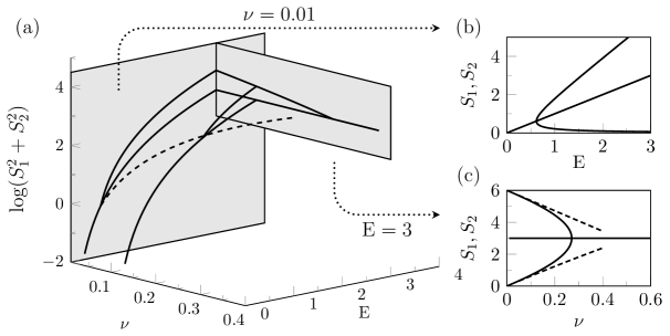
Figure 3: Bifurcation diagrams resulting from numerical solutions of (5) with $f=0.3$ for the case of $N=2$ spots centered at $(\phi,\theta)=(0,{\pi/2})$ and $(\phi,\theta)=(\pi,{\pi/2})$. The larger plot (a) shows the three-dimensional bifurcation structure, with $\log(S_{1}^{2}+S_{2}^{2})$ as a function of $\nu$ and $\mathrm{E}$. The dashed path corresponds to $\mathrm{E}=\sqrt{d_{0}\nu}$ where $S_{1,2}=\sqrt{d_{0}}\nu$ from (70). Individual spot strengths corresponding to fixed values of $\mathrm{E}$ and $\nu$ are shown in (b) and (c). The dashed line (c) corresponds to Type II asymmetric solutions, given from (64). To leading order they are $S_{1}\sim 2\mathrm{E}$ and $S_{2}\sim{\nu d_{0}/(2\mathrm{E})}$. In (b), the solution $S_{1}$ and $S_{2}$ to the reduced system (69), valid for $\mathrm{E}=\mathcal{O}(\nu^{1/2})$, overlays almost exactly with the full numerical solution.

For a fixed value of $\mathrm{E}$, in subfigure 3(c) we plot the curves $S_{1,2}$ versus $\nu$. Note that when $N=2$, the matrix $\mathcal{G}$ is cyclic, and there exists a solution of (5) with the common spot strength, $S_{c}=2\mathrm{E}/N$. This corresponds to the flat line $S_{1,2}=3$ in the subfigure. We shall call these Type I patterns. We also see that when $\nu$ is sufficiently small, there appears to be an additional asymmetric pattern that bifurcates from the Type I branch, with one small $\mathcal{O}(\nu)$ spot and one large $\mathcal{O}(1)$ spot. We refer to these as Type II patterns. Both Type I and II solutions are studied in §4.3.

However, it is apparent from Figure 3 that there also exists a distinguished limit if $\mathrm{E}\to 0$ simultaneously as $\nu\to 0$. This is shown via the curves $(\mathrm{E},S_{1,2})$ in subplot (b). As similar to Type I and II solutions, there is a shared curve where $S_{1}=S_{2}$ (the centre curve of the subplot), and two flanking curves corresponding to a small and large spot, which bifurcate from the centre branch. In §4.3, we demonstrate that the distinguished limit is described by $\mathrm{E}=\mathcal{O}(\sqrt{\nu})$ as $\nu\to 0$, and the solutions shown in (b) near the bifurcation point correspond to spot strengths of $\mathcal{O}(\sqrt{\nu})$. We call these Type III patterns and they correspond to both equal and unequal spot strengths. We will also later derive the formula for the dashed line, $\mathrm{E}=\mathrm{E}(\nu)$ in Figure 3(a), which describes the critical bifurcation point of the $\mathrm{E},\nu\to 0$ limit, where the asymmetric branches split from symmetric branch.

For $N>2$, the situation is more complex in the case of the asymmetric Type II patterns, and there may be $m<N$ spots of strength $\mathcal{O}(1)$ and $(N-m)$ spots of strength $\mathcal{O}(\nu)$. However, the classification remains the same, and we can expect the following three types of solutions:

Type I (symmetric): $$S_{j}=\mathcal{O}(1), j=1,2,\ldots,N,$$ (57)

Type II (asymmetric): $$S_{j}=\Bigg{\{}\begin{aligned} &\mathcal{O}(1),\\ &\mathcal{O}(\nu),\end{aligned} \!\begin{aligned} j&=1,2,\ldots,m,\\ j&=m+1,\ldots,N,\end{aligned}$$

Type III (a/symmetric): $$S_{j}=\mathcal{O}(\nu^{1/2}), j=1,2,\ldots,N.$$

We now comment on the splitting of the asymmetric branches from the symmetric branches for general number of spots. If the spot locations, $\bm{x}_{j}$, for $j=1,\ldots,N$ are distributed in such a way that

$$\mathcal{G}\bm{e}=k_{1}\bm{e}\,,$$ (58)

then a solution to (5) is the equal spot-strength solution $\bm{S}=S_{c}\bm{e}$ where

$$S_{c}=\frac{2\mathrm{E}}{N}\,.$$ (59)

The property (58) holds for any two-spot pattern, for a pattern of equally spaced spots on a ring of constant latitude, for spots centered at the vertices of any of the platonic solids (see Table 1 of [32] and §5 below).

Assuming that $N>1$ and that (58) holds, then a bifurcation occurs if and only if the Jacobian matrix of $\mathcal{N}(\bm{S})$ in (5) is singular when $\bm{S}=S_{c}\bm{e}$. By setting $\bm{S}=S_{c}\bm{e}+\bm{\Phi}$, with $|\bm{\Phi}|\ll 1$ in (5), a bifurcation from the symmetric solution branch occurs if and only if there exists a non-trivial $\bm{\Phi}$ to

$$\Bigl{[}\bm{\mathrm{I}}-\nu(\bm{\mathrm{I}}-{\mathcal{E}}_{0})(\mathcal{G}-\chi^{\prime}(S_{c})\bm{\mathrm{I}})\Bigr{]}\bm{\Phi}=0\,.$$ (60)

Upon comparing (60) with (53), we observe that this bifurcation point corresponds to a zero-eigenvalue crossing, and hence an exchange of stability for the symmetric solution branch. Since $\mathcal{G}$ is a symmetric matrix with $\mathcal{G}\bm{e}=k_{1}\bm{e}$, it follows that there exists eigenvectors, $\bm{q}_{j}$, with $\mathcal{G}\bm{q}_{j}=k_{j}\bm{q}_{j}$, for $j=2,\ldots,N$, where $\bm{q}_{j}^{T}\bm{e}=0$. It is readily verified that $\bm{\Phi}=\bm{q}_{j}$ satisfies (60) when $S_{c}=S_{c_{j}}$ for $j=2,\ldots,N$, where $S_{c_{j}}$ satisfies the nonlinear algebraic equation

$$\nu^{-1}-k_{j}+\chi^{\prime}(S_{c_{j}})=0\,,\qquad j=2,\ldots,N\,.$$ (61)

From (59), this indicates that a bifurcation occurs at the $j=2,\ldots,N$ points where

$$\mathrm{E}=\mathrm{E}_{j}=\frac{NS_{c_{j}}}{2}.$$ (62)

For $\nu\ll 1$, this yields $\mathrm{E}_{j}={\mathcal{O}}(\nu^{1/2})$.

Note, however, that it may be the case that the eigenvalues, $\bm{q}_{j}$, are not distinct, and in particular, this can certainly occur if, e.g. the spots are arranged on a plane of constant latitude and $\mathcal{G}$ is a cyclic matrix. In this case, the number of bifurcating branches will still be $N-1$, but the number of bifurcation points (in $\mathrm{E}$) will be equal to the number of distinct eigenvalues. In §4.4, we will derive the dashed curve $\mathrm{E}=\mathrm{E}(\nu)$ shown in Figure 3(a), which is a case of (62) in the uniform limit of $\mathrm{E}\to 0$ and $\nu\to 0$, and where the bifurcation points coalesce.

4.3 Quasi-equilibria for $\mathrm{E}=\mathcal{O}(1)$ (Type I and II)

We first consider the symmetric Type I patterns, for which all spots are characterized by $S_{j}=\mathcal{O}(1)$. For $\nu={-1/\log\epsilon}\ll 1$, a two-term regular perturbation expansion of (5) yields that

$$\bm{S}\sim\frac{2E}{N}\left[\bm{e}+\nu(\bm{\mathrm{I}}-{\mathcal{E}}_{0}){\mathcal{G}}\bm{e}+{\mathcal{O}}(\nu^{2})\right]\,.$$ (63)

Here $\bm{S}=(S_{1},\ldots,S_{N})^{T}$, $\bm{e}=(1,\ldots,1)^{T}$, ${\mathcal{E}}_{0}$ and ${\mathcal{G}}$ are defined in Principal Result 1.

To determine the stability property of Type I patterns, we observe from (48) that ${\mathcal{M}}=I+{\mathcal{O}}(\nu)$ as $\nu\to 0$ when $\bm{S}={\mathcal{O}}(1)$ and $\lambda={\mathcal{O}}(1)$. In addition, from (52), we have ${\mathcal{M}}_{0}=I+{\mathcal{O}}(\nu)$ for $\lambda=0$. As such, since both $\mathcal{M}$ and $\mathcal{M}_{0}$ are non-singular for $\nu\to 0$ when $\bm{S}={\mathcal{O}}(1)$, we conclude from the GCEP criterion in Principal Result 3 that this class of spot pattern is linearly stable to radially symmetric perturbations near each spot when $\nu\ll 1$. As such, the stability criterion for this class of solutions is simply that $S_{j}<\Sigma_{2}(f)$ to prevent spot self-replication instabilities triggered by a locally non-radially symmetric perturbation near the $j^{\textrm{th}}$ spot.

Next, consider Type II patterns. Suppose that there are $m\geq 1$ small spots, with $S_{j}={\mathcal{O}}(\nu)$ for $j=1,\ldots,m$, and $N-m$ large spots with $S_{j}={\mathcal{O}}(1)$ for $j=m+1,\ldots,N$. By using $\chi(S)\sim{d_{0}/S}$ as $S\to 0$ in (B.85), a perturbation calculation on (5) shows that the spot-strengths for this pattern have the following two-term asymptotics for $\nu\ll 1$:

$$S_{j}\sim\begin{cases}S_{0}^{\star}+\nu S_{j1}^{\star}+\cdots&\text{for $j=m+1,\ldots,N$}\\ \nu S_{0}+\nu^{2}S_{j1}+\cdots&\text{for $j=1,\ldots,m$}\end{cases}\,,$$ (64a)

where $$S_{0} S_{j1} S_{0}^{\star} S_{j1}^{\star}$$, , , and , are given by

$$S_{0}^{\star} =\frac{2\mathrm{E}}{N-m}\,, \quad S_{j1}^{\star} =-\frac{md_{0}}{2\mathrm{E}}+\frac{2\mathrm{E}}{N-m}\mathcal{L}_{j}\,,$$ (64b)

$$S_{0} =\frac{d_{0}(N-m)}{2\mathrm{E}}\,, \quad S_{j1} =\frac{d_{0}(N-m)^{2}}{8\mathrm{E}^{3}}\left[d_{0}N-2\mathrm{E}\chi(S_{0}^{\star})-\frac{4\mathrm{E}^{2}}{(N-m)}\mathcal{L}_{j}\right]\,.$$ (64c)

Here $$d_{0}={b(1-f)/f^{2}} \mathcal{L}_{j}$$ from (B.85), while is defined by

$$\mathcal{L}_{j}\equiv\sum_{\begin{subarray}{c}i=m+1\\ i\neq j\end{subarray}}^{N}L_{ij}-\frac{1}{N-m}\sum_{\begin{subarray}{c}i=m+1\\ i\neq k\end{subarray}}^{N}\sum_{k=m+1}^{N}L_{ik}\,,\qquad L_{ij}\equiv\log|\bm{x}_{i}-\bm{x}_{j}|\,.$$ (64d)

From the criterion in Principal Result 3, we now show that these Type II patterns are all unstable.

Principal Result 4 (Stability of Type II patterns).

For $\epsilon\to 0$, the Type II quasi-equilibrium patterns with spot strengths in (64) are all unstable on an ${\mathcal{O}}(1)$ time-scale.

Proof.

For $\nu\ll 1$, we show that $\mbox{det}(\mathcal{M})=0$ for some $\lambda$ on the positive real axis that is ${\mathcal{O}}(\nu)$ close to the eigenvalue $\sigma_{0}>0$ of the local operator $L_{0}$ defined in Lemma 3. We set $\lambda=\sigma_{0}-\delta_{0}\nu$ for some $\delta_{0}>0$, and look for a root of (49) where $\mathcal{M}$ is defined in (48). From (55a) and (56b) of Lemma 3, and (64), we obtain for the small spots that $B_{j}={\mathcal{O}}(\nu^{-1})$, with

$$B_{j}\sim-\frac{4\mathrm{E}^{2}}{\nu d_{0}^{2}(N-m)^{2}}\delta_{0}\hat{B}_{0-}\,,\qquad\hat{B}_{0-}\equiv\frac{(1-f)d_{0}(\sigma_{0}+1)}{\sigma_{0}+1-f}\frac{b}{2C}\,,\quad j=1,\ldots,m\,,$$ (65)

where $C>0$ is defined in (56b). In contrast, for the large spots we have $B_{j}={\mathcal{O}}(1)$ for $j=m+1,\ldots,N$. Upon substituting (65) into (48), we obtain that

$$\mathcal{M}=\bm{\mathrm{I}}-\frac{4\mathrm{E}^{2}}{d_{0}^{2}(N-m)^{2}}\delta_{0}\hat{B}_{0-}\begin{pmatrix}\bm{\mathrm{I}}_{m}&0\\ 0&0\end{pmatrix}+{\mathcal{O}}(\nu)\,,$$ (66)

where $\bm{\mathrm{I}}_{m}$ is the $m\times m$ identity matrix. Upon setting $\det(\mathcal{M})=0$, we get that $\mathcal{M}$ is singular when

$$\delta_{0}=\frac{d_{0}^{2}(N-m)^{2}}{4\mathrm{E}^{2}\hat{B}_{0-}}=\frac{d_{0}(N-m)^{2}}{2\mathrm{E}^{2}}\frac{(\sigma_{0}+1-f)C}{(1-f)(\sigma_{0}+1)b}>0\,.$$ (67)

Thus, for Type II patterns the GCEP has an eigenvalue $\mbox{Re}(\lambda)>0$ with asymptotics $\lambda=\sigma_{0}-{\mathcal{O}}(\nu)$. ∎

4.4 Quasi-Equilibria for $\mathrm{E}={\mathcal{O}}(\sqrt{\nu})$ (Type III patterns)

As shown in Fig. 3, there exists a distinguished limit when both $\mathrm{E}$ and $\nu\to 0$ simultaneously, leading to Type III patterns. The correct scaling that captures this limit is $\mathrm{E}=\mathcal{O}(\sqrt{\nu})$ and we introduce the re-scaled new variables $\tilde{S}_{j}$, $\tilde{E}$, and $\tilde{v}$, defined by

$$S_{j}=\tilde{S}_{j}\nu^{1/2}\,,\qquad\mathrm{E}=\tilde{\mathrm{E}}\nu^{1/2}\,,\qquad v_{c}=\tilde{v}\nu^{1/2}\,,$$

into the alternative form (26a) of the nonlinear system for the spot strengths. Upon using $\chi(S_{j})\sim{d_{0}/S_{j}}$ as $S_{j}\to 0$ from (B.85), we obtain that $\tilde{S}_{j}$ for $j=1,\ldots,N$ and $\tilde{v}$ satisfy the leading-order result

$${\mathcal{H}}(S_{j})\equiv\tilde{S}_{j}+\frac{d_{0}}{\tilde{S}_{j}}=\tilde{v}\,,\qquad\sum_{j=1}^{N}\tilde{S}_{j}=2\tilde{\mathrm{E}}\,,$$ (68)

where $d_{0}$ is given in (B.85). The function ${\mathcal{H}}(\xi)$ in (68) is convex for $\xi>0$ and satisfies ${\mathcal{H}}(\xi)\to+\infty$ as $\xi\to 0^{+}$ and as $\xi\to\infty$. It has a global minimum at $\xi=\sqrt{d_{0}}$ with minimum value ${\mathcal{H}}(\sqrt{d_{0}})=2\sqrt{d_{0}}$.

With these properties of ${\mathcal{H}}(\xi)$, it follows that each spot can either be of small spot strength, $\tilde{S}_{-}$, or large spot strength, $\tilde{S}_{+}$, where $0<\tilde{S}_{-}\leq\sqrt{d_{0}}\leq\tilde{S}_{+}$. To construct an asymmetric pattern with $N_{-}$ small spots and $N_{+}=(N-N_{-})$ large spots, we must solve the leading-order problem

$${\mathcal{H}}(\tilde{S}_{-})={\mathcal{H}}(\tilde{S}_{+})\,,\qquad N_{-}\tilde{S}_{-}+(N-N_{-})\tilde{S}_{+}=2\tilde{E}\,.$$ (69)

The bifurcation point where asymmetric quasi-equilibria emerge from the common spot strength solution branch is obtained by setting $N_{-}=0$ and $\tilde{S}_{-}=\tilde{S}_{+}$, which yields

$$\tilde{E}\sim\frac{N\sqrt{d_{0}}}{2}\quad\text{and}\quad\tilde{S}_{-}=\tilde{S}_{+}\sim\sqrt{d_{0}}\,.$$ (70)

For different $N_{-}$ and $N_{+}$, in Fig. 4 we plot $\sum_{j=1}^{N}\tilde{S}_{j}^{2}$ versus $\tilde{E}$, as computed from (69), illustrating the symmetric and asymmetric solution branches.

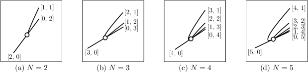
Figure 4: Bifurcation diagrams for the leading-order problem (69). The horizontal axis corresponds to $\tilde{\mathrm{E}}$ and the vertical axis to the solution measure $(\tilde{S}_{1}^{2}+\ldots\tilde{S}_{N}^{2})$. The circular nodes correspond to where asymmetric branches bifurcate from the symmetric solution branch. The notation corresponds to $[N_{-},N_{+}]$, the number of $\tilde{S}_{-}$ and $\tilde{S}_{+}$ spots.

Notice furthermore that the asymmetric branches for (69) that emerge from the bifurcation point (with the symmetric branch) can be continued into the regime where $\tilde{E}={\mathcal{O}}(\nu^{-1/2})$, or equivalently where $\mathrm{E}={\mathcal{O}}(1)$. These lead to the unstable Type II mixed patterns studied in §4.3, which consist of both small and large spots. This is the connection between the two shaded planes in Fig. 3.

However, the question of whether the prediction of a common bifurcation point from this leading-order system (69) is robust to perturbations in $\nu$ from the full system (5) is another matter entirely, and is found to depend on whether the condition (58) on the Green’s matrix holds or not (see Fig. LABEL:fig:auto_N3). When (58) holds, (61) will be used below in (71) to show that, for $N>2$, higher order in $\nu$ terms lead to transcritical bifurcation points in $\mathrm{E}$ that are ${\mathcal{O}}(\nu^{3/2})$ close.

4.5 Comparisons with numerical results

The conclusion from our analysis in §4.2 and from Fig. 3 regarding the global bifurcation structure for $N=2$ is as follows. First, for $N=2$, the common solution with $\bm{S}=\mathrm{E}\bm{e}$ is an exact solution for all $\nu$ for any two-spot pattern. This follows since $\mathcal{G}$ is cyclic for any two-spot configuration. Second, in the limit $\nu\to 0$ with $\mathrm{E}={\mathcal{O}}(1)$, the Type II patterns are given by setting $m=1$ and $N=2$ in (64). Third, for $\nu\to 0$ with $\mathrm{E}={\mathcal{O}}(\nu^{1/2})$ the asymmetric quasi-equilibrium is characterized by (69), and indeed bifurcates from the symmetric solution branch for any $\nu>0$ small. This bifurcation, calculated from (70), is shown in the dashed curve in Fig. 3(a).

Recall from §4.2 that whenever the Green’s matrix $\mathcal{G}$ satisfies (58) there is a solution (for all $\nu$) where the spots have a common strength. Typically, there is a degenerate eigenvalue for $\mathcal{G}$ of multiplicity two in the subspace perpendicular to $\bm{e}$. This must necessarily be true if $\mathcal{G}$ is cyclic.

We now consider the case $N=3$ and study the effect on the bifurcation structure of solutions to (5) on whether (58) holds or not. In Figs. 5 and 6, we show numerical solutions for $f=0.3$ and $N=3$ spots of two different spatial configurations. The results in Fig. 5 correspond to when the spots are placed equidistantly along the equator, and (58) holds, while for the other figure, the spots are placed asymmetrically along the equator, so that (58) does not hold. The bifurcation curves are plotted in $(\nu,\mathrm{E},\log\|\bm{S}\|^{2}_{2})$ space.

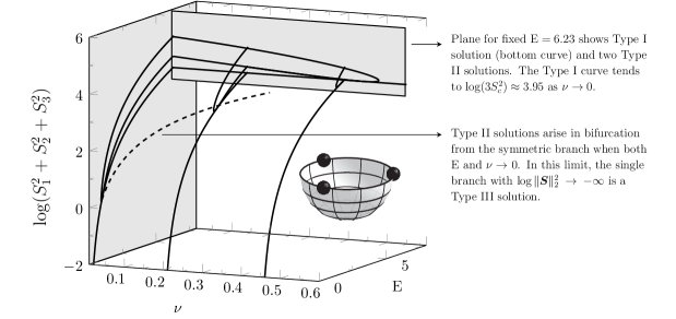
Figure 5: Bifurcation diagrams of (5) in $(\nu,\mathrm{E},\|\bm{S}\|_{2}^{2})$ space corresponding to $N=3$ and $f=0.3$. The vertical axis is $\log(S_{1}^{2}+S_{2}^{2}+S_{3}^{2})$. The spots centered symmetrically at $(\phi,\theta)=\{(0,\pi/2),(2\pi/3,\pi/2),(4\pi/3,\pi/2)\}$. For small values of $\nu$, there are two Type II patterns originating from a common bifurcation point from the symmetric solution branch in the $\mathrm{E}=\mathcal{O}(\nu^{1/2})$ regime. The two planes correspond to $\nu=0.01$ and $\mathrm{E}=6.23$.

In both configurations, when $\mathrm{E}=\mathcal{O}(1)$ is fixed, we observe two Type II patterns in the $\nu\to 0$ limit. These solutions are found by setting $(m,N)=(1,3)$ and $(m,N)=(2,3)$ in (64). For the symmetric arrangement of Fig. 5, $\bm{S}={2\mathrm{E}\bm{e}/3}$ is a solution for all $\nu>0$, and for sufficiently small $\nu$, it is observed that the Type II patterns bifurcate from the symmetric branch in the $\mathrm{E}=\mathcal{O}(\nu^{1/2})$ regime at a common bifurcation point. In the $\nu\to 0$ limit, the common bifurcation point is given by (70), and as seen in the figure, the agreement with the numerical solutions is very good. For this case, $\mathcal{G}$ is a cyclic matrix, so that there is only one eigenvalue of multiplicity two in the subspace orthogonal to $\bm{e}$. As such, from (61), there is still a common bifurcation point when higher order terms in $\nu$ are included, and indeed this is evident from the figure.

However, for the asymmetric arrangement of Fig. 6, where (58) does not hold, we observe that for any $\nu>0$ the Type II solution branch does not undergo a transcritical bifurcation when path-followed into the $\mathrm{E}=\mathcal{O}(\nu^{1/2})$ regime. This figure shows that the leading-order $\nu=0$ approximation (69), which predicts a common bifurcation point, is not robust to perturbations in $\nu>0$ and, therefore, exhibits imperfection sensitivity to higher order terms.

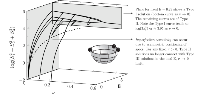
Figure 6: Same as for Fig. 5 but with spots are centered asymmetrically at $(\phi,\theta)=\{(0,{\pi/2}),({\pi/4},{\pi/2}),(\pi,{\pi/2})\}$. For small values of $\nu$, there are two Type II patterns for $\mathrm{E}=\mathcal{O}(1)$ that do not originate from transcritical bifurcations in the $\mathrm{E}=\mathcal{O}(\nu^{1/2})$ regime. The two planes correspond to $\nu=0.01$ and $\mathrm{E}=6.23$.

4.6 Stability criterion for $\mathrm{E}=\mathcal{O}(\sqrt{\nu})$ (Type III patterns)

We now return to the issue of stability discussed in §4.1, but make use of the limit $\mathrm{E},\nu\to 0$ derived in §4.4 in order to focus on the behaviour near the critical bifurcation points $\mathrm{E}=\mathrm{E}_{j}$ given in (62).

By using (56c) for $\chi^{\prime}(S_{j})$ as $S_{j}\to 0$ in (61), and then letting $\nu\to 0$, we obtain

$$\mathrm{E}_{j}\sim\frac{N\sqrt{\nu d_{0}}}{2}\left[1-\nu(d_{1}-\kappa_{j})+{\mathcal{O}}(\nu^{2})\right]\,,\qquad j=2,\ldots,N\,.$$ (71)

Again, we remark that the eigenvalues $k_{j}$ for $j=2,\ldots,N$ of $\mathcal{G}$ in the subspace perpendicular to $\bm{e}$ are in general not distinct. This eigenvalue degeneracy is necessarily the case when $\mathcal{G}$ is a cyclic matrix. In this case, the number of bifurcating branches is $N-1$, but the number of bifurcation points in $\mathrm{E}$ is the number of distinct $k_{j}$ in $j=2,\ldots,N$.

From (71), the leading-order stability threshold is $\mathrm{E}\sim\mathrm{E}_{c}$ with $\mathrm{E}_{c}\equiv{N\sqrt{\nu d_{0}}/2}={\mathcal{O}}(\sqrt{\nu})$. To analyze the zero eigenvalue crossing as $\mathrm{E}$ crosses above $\mathrm{E}_{c}$, we use (52) together with $\mathcal{B}\sim-\hat{B}_{0}S_{c}^{-2}\bm{\mathrm{I}}$ for $S_{c}={2\mathrm{E}/N}\ll 1$, to get for $\lambda\ll 1$ that

$$\mathcal{M}_{0}\bm{q}_{j}=\bm{q}_{j}-\nu\left(\bm{\mathrm{I}}-\frac{\mu}{1+\mu}{\mathcal{E}}_{0}\right)\left(\mathcal{G}-\mathcal{B}\right)\bm{q}_{j}=\left(1-\nu\kappa_{j}+\nu\frac{\hat{B}_{0}}{S_{c}^{2}}\right)\bm{q}_{j}\,,$$

where $\mathcal{G}\bm{q}_{j}=\kappa_{j}\bm{q}_{j}$ for $j=2,\ldots,N$. Therefore, $\mbox{det}(\mathcal{M}_{0})=0$ for $|\lambda|\ll 1$ when

$$\frac{1}{\nu}-\kappa_{j}+\frac{\hat{B}_{0}}{S_{c}^{2}}=0\,,$$ (72)

where $S_{c}={2\mathrm{E}/N}$ and $\hat{B}_{0}$ is defined in (55a). By solving (72) for $\mathrm{E}$, we obtain to leading order in $\nu$ that

$$\left(\frac{\mathrm{E}}{\mathrm{E}_{c}}\right)^{2}=\mathcal{Z}(\lambda)\,,\qquad\mathcal{Z}(\lambda)\equiv(1-f)\left(\frac{\lambda+1}{\lambda+1-f}\right)\frac{b}{2\mathcal{K}(\lambda)}\,.$$ (73)

Upon using the properties of $\mathcal{K}(\lambda)$ in (56a) we conclude that $\mathcal{Z}(0)=1$, and we calculate

$$\mathcal{Z}^{\prime}(\lambda)=\frac{(1-f)b}{2}\left(-\frac{f}{\mathcal{K}(\lambda)(\lambda+1-f)^{2}}-\frac{(\lambda+1)}{(\lambda+1-f)}\frac{\mathcal{K}^{\prime}(\lambda)}{\left[\mathcal{K}(\lambda)\right]^{2}}\right)<0$$ (74)

on $0<\lambda<\sigma_{0}$. Therefore, for any $\mathrm{E}<\mathrm{E}_{c}$ with $\mathrm{E}-\mathrm{E}_{c}$ small, there exists a unique $\lambda^{\star}\ll 1$ with $\lambda^{\star}>0$.

We conclude that the zero eigenvalue crossing is such that the symmetric solution branch is unstable for $\mathrm{E}<\mathrm{E}_{c}={N\sqrt{\nu d_{0}}/2}$ for $\mathrm{E}-\mathrm{E}_{c}$ small. For $\mathrm{E}>\mathrm{E}_{c}$ with $E-\mathrm{E}_{c}$ small, the spectrum of the linearization around the symmetric solution has no unstable real eigenvalues. Through the detailed analysis of a nonlocal eigenvalue problem, it was shown in §4.4 of [32] that in fact there are no unstable eigenvalues in $\mbox{Re}(\lambda)>0$, and consequently the symmetric solution branch is linearly stable when $\mathrm{E}>\mathrm{E}_{c}$ with $\mathrm{E}={\mathcal{O}}(\sqrt{\nu})$.

5 A selection of results for spot dynamics

In this section we give some results for spot dynamics as obtained by solving the DAE system (9) and (5) numerically with $\mathrm{E}={\mathcal{O}}(1)$. Based on the stability analysis of §4, we only consider patterns for which $S_{j}={\mathcal{O}}(1)$ as $\nu\to 0$. The slow dynamics (9) is valid provided that each $S_{j}$ is below the spot self-replication threshold, i.e. $S_{j}<\Sigma_{2}$ for $j=1,\ldots,N$. For a two-spot pattern the following result, as proved in C.4, provides an explicit solution to the DAE system:

Lemma 4 (Explicit two-spot solution).

Let $\gamma_{1,2}=\gamma_{1,2}(\sigma)$ denote the angle between the spot centers $\bm{x}_{1}$ and $\bm{x}_{2}$, i.e. $\bm{x}_{2}^{T}\bm{x}_{1}=\cos\gamma_{1,2}$. Then, provided that $E<\Sigma_{2}(f)$, we have for all time $\sigma=\epsilon^{2}t\geq 0$ that

$$\cos\left({\gamma_{1,2}/2}\right)=\cos\left({\gamma_{1,2}(0)/2}\right)e^{-{\mathrm{E}\sigma/|{\mathcal{A}}(\mathrm{E})|}}\,.$$ (75)

Since $\gamma_{1,2}\to\pi$ as $\sigma\to\infty$ for any $\gamma_{1,2}(0)$, the steady-state two-spot pattern will have spots centered at antipodal points on the sphere for any initial configuration of spots.

Before proceeding, we also note that in in (8) and (9), the spot locations are coupled to the spot strengths by (5). One key feature of the DAE system (9) and (5) is that it is invariant under an orthogonal transformation. The following lemma, proved in C.5, will be used in §5 for classifying equilibria of this DAE system:

Lemma 5 (Invariance under orthogonal transformations).

Suppose that $\bm{x}_{j}(\sigma)$ for $j=1\,,\ldots,N$ is the solution to the DAE system (9) and (5) with $\bm{x}_{j}(0)=\bm{x}_{j}^{0}$ for $j=1,\ldots,N$. Let $\mathcal{R}$ be any time-independent orthogonal matrix. Now let $\bm{\xi}_{j}(\sigma)$ satisfy (9), (5) with $\bm{\xi}_{j}(0)=\mathcal{R}\bm{x}_{j}^{0}$ for $j=1,\ldots,N$. Then, $\bm{\xi}_{j}(\sigma)=\mathcal{R}\bm{x}_{j}(\sigma)$ for all $j=1,\ldots,N$.

We emphasize that results similar to the DAE dynamics (5) and (9) can be derived for other RD systems. In D, we give a corresponding result for the Schnakenberg model.

5.1 Steady-state patterns from random initial arrangements

To determine the dynamics and possible equilibrium spot configurations for $N>2$ when $\mathrm{E}={\mathcal{O}}(1)$, $f$, and $\nu$ are given, we performed numerical simulations of the DAE system (9) and (5) for both pre-specified and randomly generated initial conditions for the spot locations. In the simulations in this section we used $f=0.5$ and ${\displaystyle\varepsilon}=0.02$. It is important to emphasize that for any pattern for which the spot strengths have a common value, it follows from (9) and (5) that the steady-state spatial configurations of spots are independent of $\mathrm{E}$, $f$, and $\nu$. In this sense, this restricted class of common spot-strength equilibria are universal for the Brusselator, and for other RD systems such as the Schnakenberg model. The corresponding similar DAE dynamics for the Schnakenberg model is given in (D.98) of D.

To generate a set of $N$ initial points that are uniformly distributed with respect to the surface area on the sphere, we let $h_{\phi}$ and $h_{\theta}$ be uniformly distributed random variables in $(0,1)$ and define spherical coordinates $\phi=2\pi h_{\phi}$ and $\theta=\cos^{-1}(2h_{\theta}-1)$. For the initial set of $N$ points, Newton’s method was used to solve (5) for the initial spot strengths, where the initial guess for the iteration was taken to be the two-term asymptotics (63). If the Newton iteration scheme failed to converge, indicating that no quasi-equilibrium exists for the initial configuration of spots, a new randomly generated initial configuration was generated. The DAE dynamics was then implemented by using an adaptive time-step ODE solver coupled to a Newton iteration scheme to compute the spot strengths.

Our simulations of fifty randomly generated initial spot configurations for the case $N=3$ suggests that a stable equilibrium configuration consists of three equally spaced spots that lie on a plane through the center of the sphere. The eventual colinearity and equal spacing between the three spot locations as time increases was ascertained by monitoring the distances between any two spots together with the triple product $\bm{x}_{1}\cdot(\bm{x}_{2}\times\bm{x}_{3})$ at each time step. As the slow time $\sigma$ increased, the spots became equally spaced and the triple product tended to zero. By using Lemma 5, this co-planar steady-state three-spot configuration can be mapped by an orthogonal matrix to the standard reference configuration of three equally spaced spots on the equator, i.e. $\bm{x}_{j}=(\cos({2\pi j/3}),\sin({2\pi j/3},0)^{T}$ for $j=0,1,2$. Such a standard pattern, for which (58) holds and $\bm{S}={2\mathrm{E}\bm{e}/3}$, can be readily verified analytically to be a steady-state solution for the dynamics (9).

For $N=4$, our simulations of fifty randomly generated initial spot configurations for the DAE dynamics suggests that the stable equilibrium configuration generically consists of four spots centered at the vertices of a regular tetrahedron. This was determined by showing that as time increases, the distance between any two spots tended to the common value $\sqrt{8/3}$ and that the volume $V_{\sigma}$ of the tetrahedron formed by the spot locations, given by

$$V_{\sigma}=\frac{|(\bm{x}_{1}-\bm{x}_{4})\cdot\left[(\bm{x}_{2}-\bm{x}_{4})\times(\bm{x}_{3}-\bm{x}_{4})\right]|}{6}\,,$$

tended to the volume ${8\sqrt{3}/27}$ of a regular tetrahedron. Although our random simulations suggest that a regular tetrahedron has a large basin of attraction for the dynamics of the DAE system (9) and (5), it cannot preclude the possibility of other stable steady-state configurations with much smaller basins of attraction.

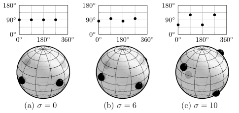
Figure 7: For $f=0.5$, $\mathrm{E}=8$, ${\displaystyle\varepsilon}=0.02$, four equally spaced spots on a ring are perturbed by a $1\%$ random perturbation in their locations. At $\sigma=6$ the spots have moved off of the ring, and at $\sigma=10$ the spots become centered at the vertices of a regular tetrahedron. The top subplots show the patterns in the $(\phi,\theta)$ plane.

For any $N\geq 2$, a ring solution, consisting of $N$ equally spaced spots on an equator of the sphere, is a steady-state solution to the DAE system (9) and (5). For $N=3$, our numerical computations suggest that such a ring solution is orbitally stable to small random perturbations in the spot locations in the sense that as time increases the perturbed spot locations will become colinear on a nearby (tilted) ring. However, for $N\geq 4$, our numerical simulations show that a ring solution is dynamically unstable to small arbitrary perturbations in the spot locations on the ring. For $N=4$, $\mathrm{E}=8$, $f=0.5$, and ${\displaystyle\varepsilon}=0.02$, in Fig. 7 we show that four spots on a ring with an initial random perturbation of $1\%$ in the spot locations will eventually tend to a regular tetrahedron as time increases.

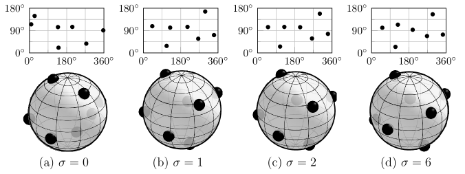
Figure 8: For $f=0.5$, $\mathrm{E}=14$, ${\displaystyle\varepsilon}=0.02$., seven spots, randomly generated, tend to an $(N-2)+2$ pattern. The pattern with $\sigma=6$ is near the steady-state. The top subplots show the patterns in the $(\phi,\theta)$ plane.

For $N=5$, $N=6$, and $N=7$, our numerical simulations employing fifty randomly generated initial spot configurations for the DAE dynamics suggests that the stable equilibrium configuration generically consists of a pair of antipodal spots, while the remaining $N-2$ spots are equally spaced on the mid-plane between these two spots. We refer to such patterns as $(N-2)+2$ patterns. The diagnostics used to form this conclusion are as follows. For each initial condition, we solved the DAE dynamics until a steady-state was reached. From this steady-state configuration two antipodal spots, labelled by $\bm{x}_{1}$ and $\bm{x}_{2}=-\bm{x}_{1}$, were identified from a dot product. We arbitrarily chose $\bm{x}_{1}$ to map to $\bm{\xi}_{1}=(0,0,1)^{T}$. We then chose any one of the other $N-2$ spots locations, such as $\bm{x}_{3}$, and map $\bm{x}_{3}$ to $\bm{\xi}_{3}=(1,0,0)^{T}$. We define $\mathcal{R}$ to be the orthogonal matrix where the first row is $\bm{x}_{3}$, the second row is ${(\bm{x}_{1}\times\bm{x}_{3})/|\bm{x}_{1}\times\bm{x}_{3}|}$, and then third row is $\bm{x}_{1}$. With this choice for the matrix $\mathcal{R}$, we found that the computed steady-state points $\bm{x}_{j}$, for $j=1\ldots,N$, can be mapped to the standard reference configuration for an $(N-2)+2$ pattern consisting of spots at $(0,0,1)$ and $(0,0,-1)$, and $N-2$ spots equally spaced on the equator $\theta={\pi/2}$ with one of these spots at $(1,0,0)^{T}$. This mapping technique was fully automated and allowed us to identify the final steady-state pattern computed from the DAE dynamics. For $N=7$, the numerical results shown in Fig. 8 illustrate the formation of the $(N-2)+2$ pattern from a random initial condition for the parameter set $f=0.5$, $\mathrm{E}=14$, and ${\displaystyle\varepsilon}=0.02$. The $(N-2)+2$ structure is evident from Fig. 8(d), which is close to the steady-state pattern. When $N=6$, the $(N-2)+2$ pattern is simply an octahedron.

For an $(N-2)+2$ pattern, the two anitipodal spots have strength $S_{p}$ while the remaining $(N-2)$ equally-spaced spots on the equator have strength $S_{c}$. By partitioning the Green’s matrix in (5) into a cyclic $(N-2)\times(N-2)$ sub-block consisting of spot interactions on the ring, we can derive after some algebra from (5) that $S_{c}$ satisfies the scalar nonlinear algebraic equation

$$\begin{gathered}S_{c}-\frac{2\nu}{N}S_{c}\left[\log(N-2)-\frac{(N-2)}{2}\log{2}\right]+\frac{2\nu}{N}\left[\chi(S_{c})-\chi(S_{p})\right]-\frac{2\mathrm{E}}{N}=0\,,\\ S_{p}=\mathrm{E}-\frac{(N-2)}{2}S_{c}\,.\end{gathered}$$ (76)

For all of our numerical DAE computations for $N=5,6,7$, we verified that the spot strengths for the steady-state pattern satisfied (76).

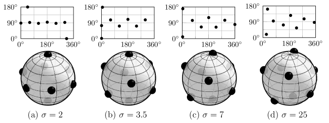
Figure 9: For $f=0.5$, $\mathrm{E}=16$, and ${\displaystyle\varepsilon}=0.02$. Eight spots in a standard $(N-2)+2$ pattern undergo a $1\%$ random perturbation at time $\sigma=0$. The initial $(N-2)+2$ pattern is found to be unstable. The pattern for $\sigma=25$ is near the steady-state pattern. The top subplots display the patterns in the $(\phi,\theta)$ plane.

Our numerical results show that the $(N-2)+2$ pattern for $N\geq 8$ is unstable. This is illustrated for $N=8$ in Fig. 9 where we took an initial $1\%$ random perturbation in the spot locations. However, unlike the cases for $N<8$ where the $(N-2)+2$ patterns were visually discernible, the final steady-state pattern in Fig. 9(d) is no longer clear. For a general steady-state configuration of $N$ points, we now propose an algorithm to rotate the sphere so that the symmetries are apparent.

Let $\Delta(\bm{x},\bm{y})>0$ be the great circle distance along the geodesic connecting the two points, $\bm{x}$ and $\bm{y}$, on the sphere. To each point, $\bm{x}$, on the sphere, we compute

$$\mathscr{D}(\bm{x})=\sum_{i=1}^{N}\Bigl{[}\Delta(\bm{x},\bm{x}_{i})^{\alpha}+\Delta(\textrm{antipodal of }\bm{x},\bm{x}_{i})^{\alpha}\Bigr{]}.$$ (77)

That is, $\mathscr{D}(\bm{x})$ is a measure of the closeness of $\bm{x}$ and its antipodal point to the set of spots. The value of $\alpha>0$ is a weighting parameter designed to penalize distance to the spots (we choose $\alpha=0.5$). Let $\bm{x}^{*}$ be an extremum (either local or global) of $\mathscr{D}$ on the sphere. We observe that by rotating the sphere so that the new north and south poles are oriented along $\bm{x}^{*}$ and its antipodal point, the symmetry patterns often become clear in the new $(\bar{\theta},\bar{\phi})$ plane. This is shown in Fig. 10 for the spot pattern in Fig. 9(d), which is now recognized as forming what we refer to as a $45^{\circ}$ “twisted cuboid”: two parallel rings containing four equally-spaced spots, with the rings symmetrically placed above and below the equator, and with the spots phase shifted by $\bar{\phi}=45^{\circ}$ between each ring. However, since the distance between the two parallel planes is not the same as the minimum distance between any two neighbouring spots on the same ring, the untwisted shape does not form a true cube. Our computations yield that the perpendicular distance between the two planes is $\approx 1.12924$ as compared to a minimum distance of $\approx 1.1672$ between neighboring spots on the same ring. The ratio of this minimum to perpendicular distance is approximately $0.967$. This yields that the rings are at latitudes $\theta\approx 55.6^{\circ}$ and $\theta\approx 124.4^{\circ}$ (see the subplot in Fig. 10).

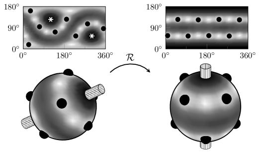
Figure 10: (Left) The same as Fig. 9(d), but the shading on the sphere and top $(\phi,\theta)$ plane show values of $\mathscr{D}(\bm{x})$, with light and dark shading for small and large values, respectively. The two asterisks (global maxima) indicate a better location to place the polar axis of the sphere (marked by a cylinder). (Right) After an orthogonal transformation, $\mathcal{R}$, the rotated sphere in the (new) $(\bar{\phi},\bar{\theta})$-plane shows two rings of four spots.

Further numerical simulations of randomly generated eight-spot patterns suggests that the stable equilibrium pattern is generically the $45^{\circ}$ degree twisted cuboid described above. Our numerical results also show that an untwisted cuboid is unstable to small random perturbations, and that a cuboid with initial twist angle $\omega$ will tend to a $45^{\circ}$ twisted cuboid as time increases.

5.2 A ring pattern with a polar spot: prediction of a triggered instability

Next, for $N\geq 3$ we consider an initial pattern with $(N-1)$ spots equidistantly spaced on a ring of constant latitude $\theta(0)$ together with a polar spot centered at $\theta=0$. For this special $(N-1)+1$ pattern, we can reduce the DAE system (5) and (9) to a scalar ODE for the latitude of the ring coupled to a single nonlinear algebraic equation for the common spot strength for the spots on the ring. For this type of pattern we will predict the occurrence of a dynamically triggered spot-splitting instability.

In terms of spherical coordinates, we have for the $N-1$ spots on the ring at time $\sigma=0$ that $\theta_{j}(0)=\theta(0)$ and $\phi_{j}(0)={2\pi(j-1)/(N-1)}$ for $j=1,\ldots,N-1$. For the polar spot, we have $\theta_{N}(0)=0$. From (8), it is readily shown that for all time, $\sigma\geq 0$

$$\phi_{j}(\sigma)=\phi_{j}(0)\,;\qquad\theta_{j}(\sigma)=\theta_{c}(\sigma)\,,\quad j=1,\ldots,N-1\,;\qquad\theta_{N}(\sigma)=0\,,$$

where $\theta_{c}(\sigma)$, with $\theta_{c}(0)=\theta(0)$, is the common latitude of the $N-1$ spots on the ring. For this pattern, the spot spot-strengths are $\bm{S}=(S_{c},\ldots,S_{c},S_{N})^{T}$, where $(N-1)S_{c}+S_{N}=2\mathrm{E}$.

The dynamics of the $(N-1)+1$ spot pattern is characterized in terms of an ODE for $\theta_{c}(\sigma)$ coupled to a nonlinear algebraic equation for $S_{c}=S_{c}(\theta_{c})$. By partitioning the Green’s matrix in (5) into a cyclic $(N-1)\times(N-1)$ sub-block consisting of spot interactions on the ring, we readily obtain from (5) that $S_{c}$ satisfies the scalar nonlinear algebraic equation

$$\mathcal{T}(S_{c})\equiv NS_{c}+\nu\left[\chi(S_{c})-\chi(S_{N})+S_{c}\left(2(N-1)L-\kappa_{N}\right)\right]-2\mathrm{E}\left(1+\nu L\right)=0\,,$$ (78a)

where $$S_{N}=2\mathrm{E}-(N-1)S_{c} L=L(\theta_{c}) L=\log|{\bm{x}}_{j}-{\bm{x}}_{N}| j=1,\ldots,N-1 \kappa_{N} (N-1)\times(N-1) {\mathcal{G}} N-1 (1,\ldots,1)^{T}$$. Here is the common value for , and is the eigenvalue of the cyclic sub-block of with corresponding dimensional eigenvector . A calculation yields that

$$L=\log\left[2\sin\left({\theta_{c}/2}\right)\right]\,,\quad\kappa_{N}=\sum_{\begin{subarray}{c}j=1\\ j\neq k\end{subarray}}^{N-1}\log|\bm{x}_{j}-\bm{x}_{k}|=\log(N-1)+(N-2)\log\left(\sin\theta_{c}\right)\,.$$ (78b)

To determine the ODE for $\theta_{c}$, we set $\theta_{j}=\theta_{c}$ for $j=1,\ldots,N-1$ in (8) to obtain that

$$\frac{\mathrm{d}\theta_{c}}{\mathrm{d}\sigma}=-(N-2)\frac{S_{c}}{\mathcal{A}(S_{c})}\cot\theta_{c}-\frac{S_{N}}{{\mathcal{A}}(S_{N})}\cot\left({\theta_{c}/2}\right)\,,\qquad\theta_{c}(0)=\theta(0)\,,$$ (79)

where $S_{N}=2\mathrm{E}-(N-1)S_{c}$. The DAE system for this pattern is to solve (79) together with the constraint $\mathcal{T}(S_{c})=0$ of (78), which yields $S_{c}=S_{c}(\theta_{c})$. As a remark, if we set $N=2$ in (78) and (79) we obtain $S_{c}=S_{N}=E$, and readily recover the two-spot dynamics of Lemma 4.

Since ${\mathcal{A}}(S_{c})<0$ and ${\mathcal{A}}(S_{N})<0$, we observe from (79) that $\theta_{c}^{\prime}>0$ for $0<\theta_{c}<{\pi/2}$, but $\theta_{c}^{\prime}<0$ as $\theta_{c}\to\pi^{-}$. As such, (79) will have a steady-state at some $\theta_{ce}$ satisfying ${\pi/2}<\theta_{ce}<\pi$.

Figure 11: Plot of the common spot strength $S_{c}$ for the $N-1$ spots on a ring (tight C-shaped curve) and the spot strength $S_{N}$ for the polar spot (open C-shaped curve) versus the ring latitude $\theta_{c}$ (in degrees), as computed from (78). The upper (lower) branch of the $S_{c}$ curve corresponds to the lower (upper) branch of the $S_{N}$ curve. The dashed portions of these curves represent quasi-equilibria that are unstable on an ${\mathcal{O}}(1)$ time-scale since $S_{N}={\mathcal{O}}(\nu)$ (see §4). The unique steady-state of the slow dynamics (79) is indicated by ${\star}$. Left panel: $f=0.5$, ${\displaystyle\varepsilon}=0.02$, $\mathrm{E}=11$, and $N=4$. Right panel: $f=0.6$, ${\displaystyle\varepsilon}=0.02$, $\mathrm{E}=14.5$ and $N=7$. In these panels, the spot self-replication thresholds $\Sigma_{2}(0.5)\approx 5.96$ and $\Sigma_{2}(0.6)\approx 4.41$ are indicated by ${\bullet}$. From the right panel, for $\theta_{c}(0)=80^{\circ}$, we predict that the polar spot with spot strength $S_{N}$ will undergo a dynamically triggered spot self-replication instability before reaching the steady-state.

In the left and right panels of Fig. 11 we plot the solutions $S_{c}$ and $S_{N}$ to (78) as a function of $\theta_{c}$ for two different parameter sets. We observe that there is a minimum latitude, depending on $\mathrm{E}$, $N$, and $f$, for which quasi-equilibria can exist, which yields a saddle-node bifurcation structure. In these figures, the upper (lower) branch of the $S_{c}$ curve corresponds to the lower (upper) branch of the $S_{N}$ curve. The dashed portions of these curves are quasi-equilibria that are unstable on an ${\mathcal{O}}(1)$ time-scale since $S_{N}={\mathcal{O}}(\nu)$ (see §4). In these figures the unique steady-state, $\theta_{ce}$, of the slow dynamics (79) is indicated by a star $({\star})$, while the spot self-replication threshold is marked by a circle $(\bullet)$.

The implication of these results for spot dynamics is as follows. For any initial value $\theta_{c}(0)<\theta_{ce}$, (79) yields $\theta_{c}^{\prime}(\sigma)>0$, so that $\theta_{c}(\sigma)$ increases monotonically towards $\theta_{ce}$. In this case, $S_{c}$ decreases while $S_{N}$ increases along the solid curves in Fig. 11 until the steady-state is reached. Alternatively, if $\theta_{c}(0)>\theta_{ce}$, then $S_{c}$ increases and $S_{N}$ decreases along the solid curves in Fig. 11 until reaching the steady-state. If at $\sigma=0$ or at any $\sigma>0$ either $S_{c}$ or $S_{N}$ exceeds the threshold $\Sigma_{2}(f)$, we predict that a spot self-replication event will occur. If the threshold is exceeded only at a later time $\sigma>0$, we refer to this instability as a dynamically triggered instability.

The plots in Fig. 11 reveal several possible dynamical behaviors. First, consider the parameter set $f=0.5$, $N=4$, $\mathrm{E}=11$, and ${\displaystyle\varepsilon}=0.02$, corresponding to the left panel of Fig. 11. For an initial angle satisfying $68^{\circ}<\theta_{c}(0)<121^{\circ}$, we observe that no spot-splitting can occur and $\theta_{c}\to\theta_{ce}\approx 109.3^{\circ}$ as $\sigma\to\infty$. For $\theta_{c}(0)<68^{\circ}$, but above the saddle-node value, we have $S_{c}>\Sigma_{2}(0.5)$ and so predict that the $3$ spots on the ring will undergo a spot self-replication process beginning at $\sigma=0$. Alternatively, for $\theta_{c}(0)>121^{\circ}$, we predict that the polar spot will undergo splitting starting at $\sigma=0$. For the parameter set $f=0.6$, $N=7$, $\mathrm{E}=14.5$, and ${\displaystyle\varepsilon}=0.02$, corresponding to the right panel of Fig. 11, we observe that a dynamically triggered instability can occur for the polar spot. To illustrate this, suppose that $\theta_{c}(0)=80^{\circ}$. Then, from the right panel of Fig. 11, it follows that $S_{N}$ will exceed the spot-splitting threshold $\Sigma_{2}(0.6)\approx 4.41$ before reaching the steady-state value. Thus, we predict that the slow dynamics will trigger, at some later time, a spot self-replication event for the polar spot.

6 Discussion

Asymptotic analysis has been used to derive a DAE system (5) and (9) characterizing the slow dynamics of localized spot solutions for the Brusselator on the sphere. When the quasi-equilibrium spot solution is linearly stable to ${\mathcal{O}}(1)$ time-scale instabilities, the system describes the motions of a collection of $N$ spots on a long time-interval of order ${\mathcal{O}}({\displaystyle\varepsilon}^{-2})$. Numerical simulations of the DAE system with random initial spot locations has identified stable spatial configurations with large basins of attraction for equilibrium spots with $2\leq N\leq 8$. For the case $N=8$, such a stable spot pattern is a $45^{\circ}$ twisted cuboid, consisting of four equally spaced spots on two parallel rings, with spots on the two rings phase-shifted by $45^{\circ}$, and where the rings are at the approximate latitudes $55.6^{\circ}$ and $124.4^{\circ}$.

Although our results do not address the fundamental question of how many localized spots will form starting from a small random perturbation of the spatially uniform state, our stability results in §4 can be used to give leading-order-in-$\nu$ bounds on the minimum and maximum number of spots in a stable steady-state pattern. To leading-order in $\nu$, we showed in §4 that stable spot patterns are those for which all individual spot strengths, $S_{j}$, tend to the common value $S_{c}$ as $\nu\to 0$ [see (63)]. Using this leading order estimate, the $N$-spot pattern is stable to spot self-replication when $N$ is large enough so that $S_{c}<\Sigma_{2}(f)$, Moreover, it is stable to a competition or overcrowding instability when $N$ is small enough so that $S_{c}>\sqrt{\nu d_{0}}$ [see §4.6]. This yields the following bounds in the limit $\nu\to 0$ on the number $N$ of stable steady-state spots:

$$\frac{2\mathrm{E}}{\Sigma_{2}(f)}<N<\frac{2\mathrm{E}}{\sqrt{\nu}}\frac{f}{\sqrt{b(1-f)}}\,.$$ (80)

For the parameter set ${\displaystyle\varepsilon}=0.075$, $f=0.8$, and $\mathrm{E}=4.0$ of Fig. 1, we use $\Sigma_{2}(0.8)\approx 2.28$ to calculate $3.51<N<10.36$ from (80). The computed pattern in Fig. 1 had 6 spots. We remark that the bounds in (80) will be tighter, and hence more useful, for smaller values of $f$.

DAE systems for slow spot dynamics, similar to (5) and (9) for the Brusselator, can also be derived for other RD systems. For example, in D, we present analogous results for the Schnakenberg model. The primary feature that is needed to apply the analysis herein is that the outer approximation for the quasi-static inhibitor concentration $v$ (i.e. the long range solution component) must satisfy a linear elliptic problem on the sphere of the form $\operatorname{\Delta}_{S}v-\kappa v=A+\sum_{j=1}^{N}S_{j}\delta(\bm{x}-\bm{x}_{j})$, for some $\kappa\geq 0$ and constant $A$.

Finally, we compare our result for spot dynamics with the well-known results for the dynamics of a collection of point vortices centered at $\bm{x}_{i}$, for $i=1,\ldots,N$, on the sphere for Euler’s equations. For $N$ such point vortices of strength $\Gamma_{i}$, for $i=1,\ldots,N$, the ODE point vortex dynamics are (cf. [3], [25])

$$\bm{x}_{j}^{\prime}=\frac{1}{2\pi}\sum_{\begin{subarray}{c}i=1\\ i\neq j\end{subarray}}^{N}\Gamma_{i}\frac{\bm{x}_{i}\times\bm{x}_{j}}{|\bm{x}_{i}-\bm{x}_{j}|^{2}}\,,\qquad j=1,\ldots,N\,,$$ (81)

subject to $\sum_{i=1}^{N}\Gamma_{i}=0$. In terms of spherical coordinates, (81) for $j=1,\ldots,N$ becomes

$$\frac{\mathrm{d}\theta_{j}}{\mathrm{d}t} =-\frac{1}{4\pi}\sum_{\begin{subarray}{c}i=1\\ i\neq j\end{subarray}}^{N}\frac{\Gamma_{i}}{1-\cos\gamma_{ij}}\sin\theta_{i}\sin(\phi_{j}-\phi_{i})\,,$$ (82a)

$$\sin\theta_{j}\frac{\mathrm{d}\phi_{j}}{\mathrm{d}t} =\frac{1}{4\pi}\sum_{\begin{subarray}{c}i=1\\ i\neq j\end{subarray}}^{N}\frac{\Gamma_{i}}{1-\cos\gamma_{ij}}\left[\sin\theta_{j}\cos\theta_{i}-\cos\theta_{j}\sin\theta_{i}\cos(\phi_{j}-\phi_{i})\right]\,,$$ (82b)

where $\gamma_{ij}$ is the angle between $\bm{x}_{i}$ and $\bm{x}_{j}$. In contrast to our result for slow spot dynamics, the ODE system (82) is Hamiltonian. This structure has been used for analyzing (82) for specific problems such as, the stability of a latitudinal ring of vortices (cf. [2]), the integrable $3$-vortex problem (cf. [15]), and characterizing relative equilibria of point vortex configurations (cf. [26]).

Our asymptotic result (8) and (9) for slow spot dynamics differs in at least two key aspects from the point vortex dynamics of (81) and (82). Firstly, in (8) and (9), the spot strengths $S_{j}$ are not pre-specified, but instead are coupled to the slow dynamics by the nonlinear algebraic constraint (5). This leads to an ODE-DAE system for slow spot dynamics. In contrast, for the point vortex problem, the vortex strengths $\Gamma_{i}$ are arbitrary, subject only to the constraint that $\sum_{i=1}^{N}\Gamma_{i}=0$. Secondly, the results in (8) and (9) are asymptotically valid only when the quasi-equilibrium profile in (4) is linearly stable to ${\mathcal{O}}(1)$ time-scale instabilities. One such instability leads to the triggering of a nonlinear spot self-replication event, and this instability occurs whenever the local spot strength $S_{j}$ exceeds a threshold $\Sigma_{2}=\Sigma_{2}(f)$ (cf. [32]). A discussion of these instabilities and their implications on slow spot dynamics was discussed in §4. There is no comparable phenomena for the point vortex problem.

6.1 Open problems

We now discuss several possible directions that warrant further investigation.

6.1.1 Equilibria and the Green’s matrix

One central issue concerns the Green’s matrix, $\mathcal{G}$, appearing in the nonlinear algebraic system (5). When the spots are distributed in such a way that $\bm{e}$ is an eigenvector of $\mathcal{G}$, we have been able to expose the bifurcation structure of the solutions for the spot strengths (see §4.2). For this case, there is a solution to (5) where the spots have a common spot strength, and the number of distinct bifurcation points (in $\mathrm{E}$) from this symmetric solution branch in the $\mathrm{E}={\mathcal{O}}(\nu^{1/2})$ regime is the number of distinct eigenvalues of $\mathcal{G}$ in the subspace orthogonal to $\bm{e}$. Although it is easy to verify that $\bm{e}$ is an eigenvalue of $\mathcal{G}$ for some simple spatial arrangements of spot patterns such as, equally-spaced spots on a ring of constant latitude, spots centered at the vertices of any platonic solid (see Table 1 of [32]), or eight spots forming a twisted cuboid, it is an open problem to numerically classify all spot configurations for which $\bm{e}$ is an eigenvector of $\mathcal{G}$. For larger values of $N$, it was shown in Table 2 of [32] that the elliptic Fekete points, defined as the point set that globally minimizes the discrete logarithmic energy $V\equiv-\sum\sum_{i\neq j}\log|\bm{x}_{i}-\bm{x}_{j}|$ with $|\bm{x}_{i}|=1$, generates a Green’s matrix $\mathcal{G}$ for which $\bm{e}$, as measured in the $L_{2}$ norm, is rather close to an eigenvalue of $\mathcal{G}$. We remark that if we set $S_{j}=S_{c}$ for $j=1,\ldots,N$ in (9), then any stable steady-state solution of (9) must correspond to a local minimum of the discrete logarithmic energy. By calculating the discrete logarithmic energy of our $45^{\circ}$ twisted cuboid, and then examining Table 1 of [33], we have verified that our 8-spot twisted cuboid is indeed an elliptic Fekete point set and not just a local minimum of the discrete logarithmic energy. These observations suggest that it would be interesting to carefully examine the relation between elliptic Fekete points and equilibria of (5) and (9).

We further remark that when $\bm{e}$ is an eigenvector of $\mathcal{G}$, the steady-state spot locations for an $N$-spot pattern, having spots of a common spot strength, are independent of the parameters in the RD model. A similar universality result holds for common spot strength patterns in the Schnakenberg model (see (5) of D).

Another open problem is to use numerical bifurcation software to path-follow the small amplitude weakly nonlinear spatial patterns, which emerge from a Turing bifurcation when $\epsilon=O(1)$, into the regime $\epsilon\ll 1$ of localized spot patterns studied in this paper. In particular, as $\epsilon$ is varied, do our localized spot patterns arise from subcritical bifurcations of the weakly nonlinear amplitude equations?

6.1.2 Bifurcations and imperfection-sensitivity

However, when $\bm{e}$ is not an eigenvalue of $\mathcal{G}$, our numerical investigation for $N=3$ of the solution set to the constraint (5), has shown the qualitatively new result that the leading-order-in-$\nu$ bifurcation diagram in the $\mathrm{E}={\mathcal{O}}(\nu^{1/2})$ regime is imperfection sensitive to small perturbations resulting from higher order in $\nu$ terms. This imperfection sensitivity of the bifurcation structure of (5) when $\bm{e}$ is not an eigenvalue of $\mathcal{G}$ is a qualitatively new result in the construction of spot-type patterns. Previous asymptotic constructions of asymmetric spot-type patterns for other RD models such as the Gierer-Meinhardt, Gray-Scott, or Schnakenberg models in planar 2-D domains (see [40] for a survey), were based on a leading-order-in-$\nu$ theory, and hence the effect of higher order in $\nu$ terms were not considered. For $\nu$ small and any $N>2$, it would be interesting to provide an asymptotic analysis of imperfection sensitivity for these other RD models.

An intriguing question concerns identifying and then classifying the steady-state spot configurations of the DAE system (5) and (9), as was studied in §5. Although the patterns for $N\leq 8$ were relatively easy to recognize, it would be interesting to devise a numerical algorithm based on ideas from group theory to classify into symmetry groups any stable steady-state spot patterns on the sphere when $N>8$. We note furthermore that since the DAE system does not appear to be a gradient flow, it would also be interesting to explore whether it can admit irregular dynamics for some special initial conditions, or for larger values of $N$ than we have examined. An additional open problem is to analytically perform a stability analysis of steady-state solutions of the DAE system (5) and (9).

6.1.3 Comparisons with full numerical simulations

In order to benchmark the range of validity in $\epsilon$ of the asymptotic slow-spot dynamics, we would require full numerical simulations of the Brusselator model (1) over long time intervals. Indeed, for the simpler case of the Gray-Scott model posed on a rectangular domain, results from a related DAE system were favorably compared in [6] with full numerical results computed by a finite-element software package. However, the analogous study for the sphere and for general curved surfaces remains an open question.

Currently, our method for computing the patterns shown in Fig.1 relies on an explicit time-stepping scheme using the closest-point method (c.f. references in [32]). However, such explicit schemes are inadequate for obtaining the accuracy and time-scales necessary to validate the $\epsilon\to 0$ limit, and one would require the development of an implicit numerical solver. For example, one possible numerical approach would be to use a spectral method, tailored for the sphere, coupled to implicit-explicit (IMEX) scheme for the time-stepping. The development of such a code, which could be used for comparisons with the DAE system, is beyond the scope of this paper, but we highlight this task as an important problem for future work.

Appendix A Non-dimensionalization of the Brusselator

The standard form for the Brusselator RD model is (cf. [30])

$$\partial_{T}U={\displaystyle\varepsilon}_{0}^{2}\operatorname{\Delta}_{S}U+\hat{E}-(B+1)U+U^{2}V\,,\quad\partial_{T}V=D\operatorname{\Delta}_{S}V+BU-U^{2}V\,,$$ (A.83)

where ${\displaystyle\varepsilon}_{0}^{2}\equiv{D_{U}/L^{2}}$, $D\equiv{D_{V}/L^{2}}$, and $L$ is the radius of the sphere. Here $\operatorname{\Delta}_{S}$ is the surface Laplacian for the unit sphere. We consider the singularly perturbed limit ${\displaystyle\varepsilon}_{0}\to 0$ for which $D={D_{v}/L^{2}}={\mathcal{O}}(1)$ as ${\displaystyle\varepsilon}_{0}\to 0$. In [32] it was shown that localized spot patterns for (A.83), characterized by localized regions where $U={\mathcal{O}}({\displaystyle\varepsilon}_{0}^{-1})$, exist when $\hat{E}={\mathcal{O}}({\displaystyle\varepsilon}_{0})$. We scale (A.83) so that the amplitude of the spots is ${\mathcal{O}}(1)$ as ${\displaystyle\varepsilon}_{0}\to 0$. In terms of the new variables $t$, $u$, and $v$, defined by

$$T=\frac{t}{B+1}\,,\qquad U=\frac{\sqrt{(B+1)D}}{{\displaystyle\varepsilon}_{0}}u\,,\qquad V=\frac{B}{\sqrt{(B+1)D}}{\displaystyle\varepsilon}_{0}v\,,$$

we get that (A.83) reduces to (1), where $f$, $\tau$, ${\displaystyle\varepsilon}$, and $\mathrm{E}={\mathcal{O}}(1)$ in (1) are defined by

$${\displaystyle\varepsilon}\equiv\frac{{\displaystyle\varepsilon}_{0}}{\sqrt{B+1}}\,,\qquad\tau\equiv\frac{(B+1)}{D}\,,\qquad f\equiv\frac{B}{B+1}\,,\qquad E\equiv\frac{\hat{E}}{\sqrt{(B+1)D}{\displaystyle\varepsilon}_{0}}\,.$$ (A.84)

Our non-dimensionalization of the Brusselator so that $v$ has unit diffusivity is slightly different than that used in [32]. However, the system studied in [32] can be readily mapped to (1).

Appendix B Further details of the leading-order inner solution

Given some value of $S_{j}$ and $f$, we solve (18) numerically on the truncated domain $\rho\in[0,R]$, with $R\gg 1$, where we impose the approximate conditions $U_{j0}(R)=0$ and $V_{j0}^{\prime}(R)={S_{j}/R}$. This yields solutions $U_{j0}$ and $V_{j0}$, and we approximate $\chi$ by $\chi\approx V_{j0}(R)-S_{j}\log R$. In Fig. 12 we plot $U_{j0}$ for different values of $S_{j}$ when $f=0.3$ and $R=20$. In the left panel of Fig. 13 we plot $\chi$ versus $S_{j}$ for $f=0.3$. For $S_{j}\to 0$, the asymptotic behavior of $\chi$, as derived in [32], is

$$\begin{gathered}\chi(S_{j})\sim\frac{d_{0}}{S_{j}}+d_{1}S_{j}+\cdots\,,\quad\mbox{as}\quad S_{j}\to 0\,,\\ d_{0}\equiv\frac{b(1-f)}{f^{2}}\,,\qquad d_{1}=\frac{0.4893}{1-f}-0.4698\,,\qquad b\equiv\int_{0}^{\infty}\rho w^{2}\,\mathrm{d}{\rho}\approx 4.934\,,\end{gathered}$$ (B.85)

where $w(\rho)>0$ is defined to be the unique solution of $\operatorname{\Delta}_{\rho}w-w+w^{2}=0$ with $w\to 0$ as $\rho\to\infty$. In the right panel of Fig. 13 we plot $\chi$ versus $S_{j}$ for a few $f$ values.

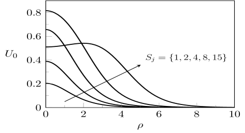
Figure 12: $U_{0}=U_{j0}(\rho)$ for $f=0.3$ and $S_{j}=\{1,2,4,8,15\}$. As $S_{j}$ increases, $U_{j0}$ develops a volcano profile.

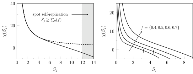
Figure 13: Left: $\chi$ versus $S_{j}$ for $f=0.3$ (heavy solid curve). The dashed curve is the asymptotic result $\chi\sim b(1-f)/(S_{j}f^{2})$ as $S_{j}\to 0$ with $b\approx 4.934$. Right: $\chi$ versus $S_{j}$ for $f=0.4$, $f=0.5$, $f=0.6$, and $f=0.7$, as shown. The thin vertical lines in these figures is the spot self-replication threshold $S_{j}=\Sigma_{2}(f)$ (see (44)). For $S_{j}>\Sigma_{2}(f)$, the quasi-equilibrium spot solution is linearly unstable on an ${\mathcal{O}}(1)$ time-scale. In this figure, the values of $f$ decrease in the direction of the arrow.

Appendix C Proofs of Lemmas

C.1 Proof to Lemma 1 (Tangent plane approximation)

We begin by letting $\bm{x}\equiv(\cos\phi\sin\theta,\sin\phi\sin\theta,\cos\theta)^{T}\equiv(f_{1},f_{2},f_{3})^{T}$, where $f_{i}=f_{i}(\phi,\theta)$ for $i=1,2,3$. By retaining the quadratic terms in the Taylor expansion of ${\bm{x}}$ as ${\bm{x}}\to{\bm{x}}_{j}$, we readily derive that

$$\bm{x}-\bm{x}_{j}\sim{\displaystyle\varepsilon}\bm{J}_{j}{\bm{s}}+\frac{{\displaystyle\varepsilon}^{2}}{2}{\bm{r}}+\cdots\,,$$ (C.86a)

where $$\bm{J}_{j} \bm{r}\equiv(r_{1},r_{2},r_{3})^{T}$$ is defined in (12b) and with components defined by

$$r_{i}\equiv\bm{s}^{T}{\mathcal{H}}_{i}\bm{s}\,,\qquad{\mathcal{H}}_{i}\equiv\begin{pmatrix}f_{i\theta\theta}&{f_{i\theta\phi}/\sin\theta}\\ {f_{i\theta\phi}/\sin\theta}&{f_{i\phi\phi}/\sin^{2}\theta}\\ \end{pmatrix}\Biggr{\rvert}_{\phi=\phi_{j},\theta=\theta_{j}}\,,\qquad i=1,2,3\,.$$ (C.86b)

The leading term in (C.86a) gives the first expression in (12a). To obtain the second relation in (12a), we calculate $$|\bm{x}-\bm{x}_{j}|^{2}\sim{\displaystyle\varepsilon}^{2}\left(\bm{s}^{T}\bm{J}_{j}^{T}\bm{J}_{j}\bm{s}+{\displaystyle\varepsilon}\bm{s}^{T}\bm{J}_{j}^{T}\bm{r}\right) \bm{J}_{j}^{T}\bm{J}_{j}=\bm{\mathrm{I}} \bm{s}^{T}\bm{s}=s_{1}^{2}+s_{2}^{2}$$. Since and , we obtain

$$|\bm{x}-\bm{x}_{j}|\sim{\displaystyle\varepsilon}\left(s_{1}^{2}+s_{2}^{2}\right)^{1/2}\left(1+\frac{{\displaystyle\varepsilon}}{2(s_{1}^{2}+s_{2}^{2})}\bm{s}^{T}\bm{J}_{j}^{T}\bm{r}\right)\,.$$ (C.86c)

Finally, we use (12b) for $\bm{J}_{j}^{T}$ and we evaluate the required partial derivatives in (C.86b) to calculate $\bm{r}$. After some lengthy, but straightforward, algebra we get that $\bm{s}^{T}\bm{J}_{j}^{T}\bm{r}=s_{1}s_{2}^{2}\cot\theta_{j}$. Upon substituting this result into (C.86c) we obtain the second result in (12a).

C.2 Proof to Lemma 2 (Static component of first-order inner solution)

The proof is by a direct verification. We set

$$\bm{U}_{1}=As_{2}^{2}\partial_{s_{1}}\bm{U}_{0}+Bs_{1}s_{2}\partial_{s_{2}}\bm{U}_{0}\,,$$ (C.87)

for some constants $A$ and $B$. For this form of $\bm{U}_{1}$ we readily calculate that

$$\operatorname{\Delta}_{(s_{1},s_{2})}\bm{U}_{1} =As_{2}^{2}\partial_{s_{1}}\left(\operatorname{\Delta}_{(s_{1},s_{2})}\bm{U}_{0}\right)+Bs_{1}s_{2}\partial_{s_{2}}\left(\operatorname{\Delta}_{(s_{1},s_{2})}\bm{U}_{0}\right)$$

$$\qquad+s_{2}\left(4A+2B\right)\partial_{s_{1}s_{2}}\bm{U}_{0}+2Bs_{1}\partial_{s_{2}s_{2}}\bm{U}_{0}+2A\partial_{s_{1}}\bm{U}_{0}\,.$$

In this expression, we use $\partial_{s_{1}}\operatorname{\Delta}_{(s_{1},s_{2})}\bm{U}_{0}=-{\mathcal{M}}\partial_{s_{1}}\bm{U}_{0}$ and $\partial_{s_{2}}\operatorname{\Delta}_{(s_{1},s_{2})}\bm{U}_{0}=-{\mathcal{M}}\partial_{s_{2}}\bm{U}_{0}$, as obtained from differentiating (31), to obtain

$$\operatorname{\Delta}_{(s_{1},s_{2})}\bm{U}_{1}=-As_{2}^{2}{\mathcal{M}}\partial_{s_{1}}\bm{U}_{0}-Bs_{1}s_{2}{\mathcal{M}}\partial_{s_{2}}\bm{U}_{0}+s_{2}\left(4A+2B\right)\partial_{s_{1}s_{2}}\bm{U}_{0}+2Bs_{1}\partial_{s_{2}s_{2}}\bm{U}_{0}+2A\partial_{s_{1}}\bm{U}_{0}\,.$$

For $\bm{U}_{1}$ of the form (C.87) we then calculate that ${\mathcal{M}}\bm{U}_{1}=As_{2}^{2}M\partial_{s_{1}}\bm{U}_{0}+Bs_{1}s_{2}{\mathcal{M}}\partial_{s_{2}}\bm{U}_{0}$. Upon adding these two expressions, we obtain

$$\mathfrak{L}\bm{U}_{1}\equiv\operatorname{\Delta}_{(s_{1},s_{2})}\bm{U}_{1}+{\mathcal{M}}\bm{U}_{1}=2s_{2}\left(2A+B\right)\partial_{s_{1}s_{2}}\bm{U}_{0}+2Bs_{1}\partial_{s_{2}s_{2}}\bm{U}_{0}+2A\partial_{s_{1}}\bm{U}_{0}\,.$$

The right hand-side of this expression agrees with that in (32a) if we choose $2A=-\cot\theta_{j}$ and $B=\cot\theta_{j}$. Finally, we calculate the far-field behavior of $V_{1}$ using (C.87). This yields $V_{1}\sim S_{j}s_{1}s_{2}^{2}{(A+B)/\rho^{2}}=S_{j}s_{1}s_{2}^{2}{\cot\theta_{j}/(2\rho^{2})}$ as $\rho\to\infty$, which agrees with (32b).

C.3 Proof to Lemma 3 (Diagonal entries of $\mathcal{B}$)

We shall derive (55) and establish (56). First, note that as $S_{j}\to 0$, the solution to the core problem (18) is given by (Principal Result 4.1 of [32])

$$U_{j0}\sim\frac{S_{j}w}{f\tilde{v}_{0}}\,,\qquad V_{j0}\sim\frac{\tilde{v}_{0}}{S_{j}}\,,\qquad\tilde{v}_{0}\equiv\frac{b(1-f)}{f^{2}}\,,$$ (C.88)

where $w(\rho)>0$ is the unique solution to $\operatorname{\Delta}_{\rho}w-w+w^{2}=0$ with $w(\infty)=0$, and $b\equiv\int_{0}^{\infty}\rho w^{2}\,\mathrm{d}{\rho}$. In (45), we then expand $\psi_{j}$, $N_{j}$ and $B_{j}$ for $S_{j}\to 0$ as

$$N_{j}=S_{j}^{-2}\left(\hat{N}_{j}+{\mathcal{O}}(S_{j}^{2})\right)\,,\quad B_{j}=S_{j}^{-2}\left(\hat{B}_{j}+{\mathcal{O}}(S_{j}^{2})\right)\,,\quad\psi_{j}=\hat{\psi}_{j}+{\mathcal{O}}(S_{j}^{2})\,.$$ (C.89)

Upon substituting (C.88) and (C.89) into (45), and collecting powers of $S_{j}$, we obtain that

$$\operatorname{\Delta}_{\rho}\hat{\psi}_{j}-\hat{\psi}_{j}+2w\hat{\psi}_{j}-\lambda\hat{\psi}_{j}=-\frac{w^{2}}{f\tilde{v}_{0}^{2}}\hat{B}_{j},\quad\hat{\psi}_{j}^{\prime}(0)=0,\quad\hat{\psi}_{j}\to 0\text{ as $\rho\to\infty$}\,,$$ (C.90a)

$$\operatorname{\Delta}_{\rho}\hat{N}_{j}=\hat{\psi}_{j}\left(\frac{2w}{f}-1\right)+\frac{w^{2}}{f^{2}\tilde{v}_{0}^{2}}\hat{B}_{j},\quad\hat{N}_{j}^{\prime}(0)=0,\quad\hat{N}_{j}\sim\log\rho+{\mathcal{O}}(1)\text{ as $\rho\to\infty$}.$$ (C.90b)

By integrating the equations for $\hat{N}_{j}$ and for $\hat{\psi}_{j}$ over $0<\rho<\infty$, we obtain that

$$\frac{2}{f}\int_{0}^{\infty}\hat{\psi}_{j}w\rho\,\mathrm{d}{\rho}-\int_{0}^{\infty}\hat{\psi}_{j}\rho\,\mathrm{d}{\rho}+\frac{\hat{B}_{j}b}{f^{2}\tilde{v}_{0}^{2}}=1\,,\qquad-(1+\lambda)\int_{0}^{\infty}\hat{\psi}_{j}\rho\,\mathrm{d}{\rho}+2\int_{0}^{\infty}w\hat{\psi}_{j}\rho\,\mathrm{d}{\rho}=-\frac{\hat{B}_{j}b}{f\tilde{v}_{0}^{2}}\,.$$ (C.91)

Upon eliminating $\int_{0}^{\infty}\hat{\psi}_{j}\rho\,\mathrm{d}{\rho}$ between these two expressions we obtain that

$$\frac{1}{f}\int_{0}^{\infty}w\hat{\psi}_{j}\rho\,\mathrm{d}{\rho}+\frac{\hat{B}_{j}b}{2f^{2}\tilde{v}_{0}^{2}}=\frac{\lambda+1}{2(\lambda+1-f)}\,.$$ (C.92)

Then, in the class of radially symmetric solutions, we write the solution, $\hat{\psi}_{j}$, to (C.90a) as

$$\hat{\psi}_{j}=-\frac{\hat{B}_{j}}{f\tilde{v}_{0}^{2}}\left(L_{0}-\lambda\right)^{-1}w^{2}\,,\qquad\mbox{where}\quad L_{0}\Phi\equiv\operatorname{\Delta}_{\rho}\Phi-\Phi+2w\Phi\,.$$ (C.93)

Finally, upon substituting (C.93) into (C.92) and solving for $\hat{B}_{j}$, we readily obtain (55) of Lemma 3.

Next, we establish (56) for $\mathcal{K}(\lambda)$ as defined in (55b). The self-adjoint problem $L_{0}\Phi=\sigma\Phi$ has a unique real eigenvalue $\sigma_{0}>0$ with eigenfunction $\Phi_{0}>0$, which we normalize as $\int_{0}^{\infty}\rho\Phi_{0}^{2}\,\mathrm{d}{\rho}=1$. Since $L_{0}^{-1}w^{2}=w$, we get $\mathcal{K}(0)=b-{b/2}={b/2}$. The monotonicity result $\mathcal{K}^{\prime}(\lambda)>0$ in (56a) for the segment $0<\lambda<\sigma_{0}$ of the real axis was proved in Appendix C of [32].

To establish the asymptotics (56b) as $\lambda\to\sigma_{0}^{-}$, we introduce $\delta>0$ small and set $\lambda=\sigma_{0}-\delta$. We then expand the solution $q$ to $(L_{0}-\lambda)q=w^{2}$ as $q=C\delta^{-1}\Phi_{0}+q_{1}+\cdots$, for some constant $C$ to be found. We obtain that $q_{1}$ satisfies $(L_{0}-\sigma_{0})q_{1}=w^{2}-C\Phi_{0}$, which has a solution only if $C=\int_{0}^{\infty}\rho w^{2}\Phi_{0}\,\mathrm{d}{\rho}$. Thus, for $\delta\ll 1$, we have $(L_{0}-\lambda)^{-1}w^{2}\sim\delta^{-1}C\Phi_{0}$. Upon substituting this expression into (55b) we obtain the asymptotics (56b) when $\lambda=\sigma_{0}-\delta$ with $\delta\ll 1$. Finally, to establish (56c), we use $B_{j}(S_{j},0)=\chi^{\prime}(S_{j})$ at each $f>0$ and the asymptotics for $\chi(S_{j})$ in (B.85) as $S_{j}\to 0$.

C.4 Proof of Lemma 4 (Explicit two-spot solution)

For any two-spot configuration $\mathcal{G}$ satisfies (58), so that from (59) we have $S_{1}=S_{2}=E$. This is the unique solution to (5) with $S_{j}={\mathcal{O}}(1)$ as $\nu\to 0$. Assume that $E<\Sigma_{2}(f)$, so that the DAE dynamics (9) is valid. We use (9) to calculate

$$\frac{\mathrm{d}|\bm{x}_{j}-\bm{x}_{i}|^{2}}{\mathrm{d}\sigma}=-2\left(\bm{x}_{2}^{T}\bm{x}_{1}^{\prime}+\bm{x}_{1}^{T}\bm{x}_{2}^{\prime}\right)=-\frac{8E}{{\mathcal{A}}(E)|\bm{x}_{2}-\bm{x}_{1}|^{2}}\left(1-(\bm{x}_{2}^{T}\bm{x}_{1})^{2}\right)\,.$$

Since $|\bm{x}_{2}-\bm{x}_{1}|^{2}=2(1-\cos\gamma_{1,2})$ and $\bm{x}_{2}^{T}\bm{x}_{1}=\cos(\gamma_{1,2})$, the expression above reduces to

$$2\sin\gamma_{1,2}\,\frac{\mathrm{d}\gamma_{1,2}}{\mathrm{d}\sigma}=-\frac{4E}{{\mathcal{A}}(E)}\left(1+\cos\gamma_{1,2}\right)=-\frac{8E}{{\mathcal{A}}(E)}\cos^{2}\left({\gamma_{1,2}/2}\right)\,.$$

Since ${\mathcal{A}}(E)<0$, this ODE is ${d\gamma_{1,2}/d\sigma}=2E{\cot\left({\gamma_{1,2}/2}\right)/|{\mathcal{A}}(E)|}$, with solution (75).

C.5 Proof of Lemma 5 (Invariance under orthogonal transformations)

The Green’s matrix $\mathcal{G}$ in the constraint (5) is invariant under $\mathcal{R}$ since $\mathcal{R}^{T}\mathcal{R}=\bm{\mathrm{I}}$ implies $|\bm{\xi}_{j}-\bm{\xi}_{i}|=|\bm{x}_{j}-\bm{x}_{i}|$ for $i\neq j$. Then, multiply (9) by $\mathcal{R}$ and use $\mathcal{R}^{T}\mathcal{R}=\bm{\mathrm{I}}$ to get

$$\frac{\mathrm{d}\mathcal{R}\bm{x}_{j}}{\mathrm{d}\sigma}=\frac{2}{\mathcal{A}_{j}}\left(\mathcal{R}-\mathcal{R}\bm{x}_{j}\bm{x}_{j}^{T}\mathcal{R}^{T}\mathcal{R}\right)\sum_{\begin{subarray}{c}i=1\\ i\neq j\end{subarray}}^{N}\frac{S_{i}\bm{x}_{i}}{|\bm{x}_{i}-\bm{x}_{j}|^{2}}\,,\qquad\mathcal{R}\bm{x}_{j}(0)=\mathcal{R}\bm{x}_{j}^{0}\,,\quad j=1,\ldots,N\,.$$

The result follows by setting $\bm{\xi}_{j}=\mathcal{R}\bm{x}_{j}$ and using $|\bm{\xi}_{j}-\bm{\xi}_{i}|=|\bm{x}_{j}-\bm{x}_{i}|$ for any $i\neq j$.

Appendix D Slow spot dynamics for the Schnakenberg model

Results similar to those in Principal Results 1 and 2 can be derived for other RD systems. Here we focus on the reduced Schnakenberg model formulated in terms of a parameter $a>0$ as

$$\frac{\partial u}{\partial t}={\displaystyle\varepsilon}^{2}\operatorname{\Delta}_{S}u-u+vu^{2}\,,\qquad\tau\frac{\partial v}{\partial t}=\operatorname{\Delta}_{S}v+a-{\displaystyle\varepsilon}^{-2}u^{2}v\,.$$ (D.94)

In place of (18), the leading-order radially symmetric inner problem near the $j^{\textrm{th}}$ spot is given by solving, for $0<\rho<\infty$, the coupled system

$$\operatorname{\Delta}_{\rho}U_{j0}-U_{j0}+U_{j0}^{2}V_{j0}=0\,,\qquad\operatorname{\Delta}_{\rho}V_{j0}-U_{j0}^{2}V_{j0}=0\,,$$ (D.95a)

$$U_{j0}^{\prime}(0)=V_{j0}^{\prime}(0)=0\,;\qquad U_{j0}\to 0\,,\ V_{j0}\sim S_{j}\log\rho+\chi+o(1)\,,\text{ as $\rho\to\infty$}\,.$$ (D.95b)

The numerically computed function $\chi=\chi(S_{j})$ is plotted in the left panel of Fig. 14.

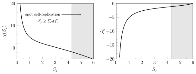
Figure 14: Schnakenberg Model. Left: $\chi(S_{j})$ versus $S_{j}$, computed from (D.95). Right: ${\mathcal{A}}_{j}$ versus $S_{j}$. The shaded regions in these figures are the regions $S_{j}>\Sigma_{2}\approx 4.3$ where the spot is unstable on an ${\mathcal{O}}(1)$ time-scale to a self-replication instability.

The other function required for the slow dynamics, and which depends on the specific form of the nonlinear kinetics, is ${\mathcal{A}}_{j}$ defined in (41). In computing ${\mathcal{A}}_{j}$ from (41), $U_{j0}$ is now given by the solution to (D.95) and $P_{1}(\rho)$ is the solution to (37) subject to $(P_{1},P_{2})^{T}\sim(0,{1/\rho})^{T}$ as $\rho\to\infty$, where the matrix ${\mathcal{M}}_{j}$ in (37) is now given in terms of the solution to (D.95) by

$${\mathcal{M}}_{j}\equiv\begin{pmatrix}-1+2U_{j0}V_{j0}&U_{j0}^{2}\\ -2U_{j0}V_{j0}&-U_{j0}^{2}\\ \end{pmatrix}\,.$$ (D.96)

The computed function ${\mathcal{A}}_{j}$ versus $S_{j}$ for the Schnakenberg model is plotted in Fig. 14. In terms of these model-specific functions $\chi(S_{j})$ and ${\mathcal{A}}_{j}$, the result for slow spot dynamics is as follows:

Principal Result 5 (Schnakenberg model: slow spot dynamics).

Let ${\displaystyle\varepsilon}\to 0$. Provided that there are no ${\mathcal{O}}(1)$ time-scale instabilities of the quasi-equilibrium spot pattern, the slow dynamics of the spot pattern on the unit sphere for (D.94) is characterized by the quasi-equilibrium solution

$$u_{\mathrm{unif}}\sim\sum_{i=1}^{N}U_{i,0}\left(\frac{|\bm{x}-\bm{x}_{i}|}{{\displaystyle\varepsilon}}\right)\,,\qquad v_{\mathrm{unif}}\sim\sum_{i=1}^{N}S_{i}L_{i}(\bm{x})+\frac{\overline{v}_{c}}{\nu}\,,$$ (D.97)

where the time-dependent spot locations $\bm{x}_{j}(\sigma)$ on the slow time-scale $\sigma$, with $\sigma={\displaystyle\varepsilon}^{2}t$, satisfy

$$\frac{\mathrm{d}\bm{x}_{j}}{\mathrm{d}\sigma}=\frac{2}{\mathcal{A}_{j}}\left(\bm{\mathrm{I}}-{\mathcal{Q}}_{j}\right)\sum_{\begin{subarray}{c}i=1\\ i\neq j\end{subarray}}^{N}\frac{S_{i}\bm{x}_{i}}{|\bm{x}_{i}-\bm{x}_{j}|^{2}}\,,\qquad{\mathcal{Q}}_{j}\equiv\bm{x}_{j}\bm{x}_{j}^{T}\,,\qquad j=1,\ldots,N\,,$$ (D.98a)

where $$S_{j} j=1,\ldots,N \overline{v}_{c} a N$$ for , and the constant in (D.97), are coupled to the spot locations and the parameter in (D.94) by the -dimensional nonlinear algebraic system

$$\mathcal{N}(\bm{S})\equiv\Bigl{[}\bm{\mathrm{I}}-\nu(\bm{\mathrm{I}}-{\mathcal{E}}_{0})\mathcal{G}\Bigr{]}\bm{S}+\nu(\bm{\mathrm{I}}-{\mathcal{E}}_{0})\bm{\chi}(\bm{S})-\frac{2a}{N}\bm{e}=\bm{0}\,,$$ (D.98b)

with $\overline{v}_{c}=2aN^{-1}+\nu N^{-1}\left(\bm{e}^{T}\bm{\chi}(\bm{S})-\bm{e}^{T}{\mathcal{G}}\bm{S}\right)$. In (D.97) and (D.98b), $L_{i}(\bm{x})\equiv\log|\bm{x}-\bm{x}_{i}|$, while the matrices ${\mathcal{G}}$, ${\mathcal{E}}_{0}$, and the vectors $\bm{\chi}$, $\bm{e}$ are as defined previously in Principal Result 1.

In [16] it was shown that the $j^{\textrm{th}}$ spot is linearly unstable on an ${\mathcal{O}}(1)$ time-scale to locally non-radially symmetric perturbations near $\bm{x}_{j}$ when $S_{j}>\Sigma_{2}\approx 4.3$. This linear instability was found in [16] to lead to a nonlinear spot self-replication event. From Fig. 14, we have ${\mathcal{A}}_{j}<0$ on $0<S_{j}<\Sigma_{2}$, so that the slow dynamics of spots is repulsive. We emphasize that the DAE system (D.98) is remarkably similar in form to that for the Brusselator model in Principal Results 1–2.

References

- [1] R. Barreira, C. A. Elliott, A. Madzvamuse, The surface finite element method for pattern formation on evolving biological surfaces, J. Math. Biol. 63, (2011), pp. 1095-1109.
- [2] S. Boatto, H. E. Cabral, Nonlinear stability of a latitudinal ring of point vortices on a non-rotating sphere, SIAM J. Appl. Math., 64(1), (2003), pp. 216–230.
- [3] V. A. Bogomolov, Dynamics of vorticity at a sphere, Fluid Dyn. (USSR), 6, (1977), pp. 863–870.
- [4] T. K. Callahan, Turing patterns with O(3) symmetry, Physica D, 188(1), (2004), pp. 65–91.
- [5] M. A. J. Chaplain, M. Ganesh, I. G. Graham, Spatio-temporal pattern formation on spherical surfaces: numerical simulation and application to solid tumour growth, J. Math. Biology, 42(5), (2001), pp. 387-423.
- [6] W. Chen, M. J. Ward, The stability and dynamics of localized spot patterns in the two-dimensional Gray-Scott model, SIAM J. Appl. Dyn. Sys., 10(2), (2011), pp. 582–666.
- [7] W. Chen, M. J. Ward, Oscillatory instabilities of multi-spike patterns for the one-dimensional Gray-Scott model, Europ. J. Appl. Math., 20(2), (2009), pp. 187–214.
- [8] P. Chossat, R. Lauterbach, I. Melbourne, Steady-sate bifurcation with symmetry, Arch. Rat. Mech. Anal., 113, (1990), pp. 313–376.
- [9] A. Doelman, W. Eckhaus, T. J. Kaper, Slowly modulated two-pulse solutions in the Gray-Scott model i: asymptotic construction and stability, SIAM J. Appl. Math., 61(3), (2000), pp. 1080-1102.
- [10] A. Doelman, W. Eckhaus, T. J. Kaper, Slowly modulated two-pulse solutions in the Gray-Scott model ii: geometric theory, bifurcations, and splitting dynamics, SIAM J. Appl. Math., 61(6), (2000), pp. 2036-2061.
- [11] A. Doelman, T. Kaper, K. Promislow, Nonlinear asymptotic stability of the semi-strong pulse dynamics in a regularized Gierer-Meinhardt model, SIAM J. Math. Anal., 38(6), (2007), pp. 1760–1789.
- [12] J. Gjorgjieva, J. Jacobsen, Turing patterns on growing spheres: the exponential case, DCDS supplement (special issue), (2007), pp. 436-445.
- [13] D. Iron, M. J. Ward, The dynamics of multi-spike solutions to the one-dimensional Gierer-Meinhardt model, SIAM J. Appl. Math., 62(6), (2002), pp. 1924-1951.
- [14] D. Iron, M. J. Ward, A metastable spike solution for a non-local reaction-diffusion model, SIAM J. Appl. Math., 60(3), (2000), pp. 778-802.
- [15] R. Kidambi, P. K. Newton, Motion of three vortices on the sphere, Physica D 116(1-2), (1998), pp. 143–175.
- [16] T. Kolokolnikov, M. J. Ward, J. Wei, Spot self-replication and dynamics for the Schnakenberg Model in a two-dimensional domain, J. Nonlinear Sci., 19(1), (2009), pp. 1–56.
- [17] T. Kolokolnikov, M. J. Ward, Reduced wave Green’s functions and their effect on the dynamics of a spike for the Gierer-Meinhardt model, Europ. J. Appl. Math., 14(5), (2003), pp. 513–545.
- [18] S. Kondo, R. Asai, A reaction–diffusion wave on the skin of the marine angelfish Pomacanthus, Nature, 376, (1995), pp. 765-768.
- [19] C. Landsberg, A. Voigt, A multigrid finite element method for reaction-diffusion systems on surfaces, Comput. Visual Sci., 13, (2010), pp. 177–185.
- [20] C. B. Macdonald, B. Merriman, S. J. Ruuth, Simple computation of reaction-diffusion processes on point clouds, Proc. Natl. Acad. Sci. U.S.A., 110(23), (2013), pp. 9209–9214.
- [21] P. C. Matthews, Pattern formation on a sphere, Phys. Rev. E., 67(3), (2003), pp. 036206.
- [22] P. C. Matthews, Transcritical bifurcation with symmetry, Nonlinearity, 16, (2003), pp. 1449-1471.
- [23] W. Nagata, L. G. Harrison, S. Wehner, Reaction-diffusion models of growing plant tips: bifurcations on hemispheres, Bull. of Math. Biology, 6(4), (2003), pp. 571–607.
- [24] Y. Nec, M. J. Ward, The stability and slow dynamics of two-spike patterns for a class of reaction-diffusion system, Math. Model. Natur. Phenom., 85, (2013), pp. 206–232.
- [25] P. K. Newton, The N-Vortex Problem: Analytical Techniques, Springer, New York, (2001).
- [26] P. K. Newton, T. Sakajo, Point vortex equilibria and optimal packings of circles on a sphere, Proc. Roy. Soc. A, 467, (2011), pp. 1468–1490.
- [27] K. J. Painter, Modelling of pigment patterns in fish: book chapter in mathematical models for biological pattern formation. editors P. K. Maini, H. G. Othmer, IMA Vol. in Math and its Applications, 121, (2000), pp. 59–82. Springer-Verlag.
- [28] B. Peña, C. Pérez-Garcia, Stability of Turing patterns in the Brusselator model, Phys. Rev. E., 64(5), (2001), pp. 056213.
- [29] R. G. Plaza, F. Sánchez-Garduño, P. Padilla, R. A. Barrio, P. K. Maini, The effect of growth and curvature on pattern formation, J. Dynam. Diff. Eq., 16(4), (2004), pp. 1093-1121.
- [30] I. Prigogine, R. Lefever, Symmetry breaking instabilities in dissipative systems. II, J. Chem. Phys., 48(4), (1968), pp. 1695-1700.
- [31] J. D. Rademacher, First and second order semi-strong interface interaction in reaction-diffusion systems, SIAM J. App. Dyn. Syst., 12(1), (2012), pp. 175–203.
- [32] I. Rozada, S. Ruuth, M. J. Ward, The stability of localized spot patterns for the Brusselator on the sphere, SIAM J. Appl. Dyn. Sys., 13(1), (2014), pp. 564–627.
- [33] W. Stortelder, J. de Swart, J. Pintér, Finding elliptic Fekete point sets: Two numerical solution approaches, J. Comput. Appl. Math. 130(1-2), (1998), pp. 205–216.
- [34] W. Sun, M. J. Ward, R. Russell, The slow dynamics of two-spike solutions for the Gray-Scott and Gierer-Meinhardt systems: competition and oscillatory instabilities, SIAM J. App. Dyn. Sys., 4(4), (2005), pp. 904–953.
- [35] W. H. Tse, M. J. Ward, Hotspot formation and dynamics for a continuum model of urban crime, Europ. J. Appl. Math., to appear, Firstview article, (2015).
- [36] J. C. Tzou, A. Bayliss, B. J. Matkowsky, V. A. Volpert, Stationary and slowly moving localized pulses in a singularly perturbed Brusselator model, Europ. J. Appl. Math., 22(5), (2011), pp. 423–453.
- [37] P. van Heijster, A. Doelman, T. J. Kaper, K. Promislow, Front interactions in a three-component system, SIAM J. Appl. Dyn. Sys., 9(2), (2010), pp. 292–332.
- [38] C. Varea, J. L. Aragón, R. A. Barrio, Turing patterns on a sphere, Phys. Rev. E., 60(4), (1999), pp. 4588-4592.
- [39] M. J. Ward, J. Wei, Hopf bifurcation of spike solutions for the shadow Gierer-Meinhardt model, 14(6), (2003), pp. 677-711.
- [40] J. Wei, M. Winter, Stationary multiple spots for reaction-diffusion systems, J. Math. Biol., 57(1), (2008), pp. 53–89.