Two-sample Bayesian nonparametric goodness-of-fit test

Abstract

In recent years, Bayesian nonparametric statistics has gathered extraordinary attention. Nonetheless, a relatively little amount of work has been expended on Bayesian nonparametric hypothesis testing. In this paper, a novel Bayesian nonparametric approach to the two-sample problem is established. Precisely, given two samples $\mathbf{X}=X_{1},\ldots,X_{m_{1}}$ $\overset{i.i.d.}{\sim}F$ and $\mathbf{Y}=Y_{1},\ldots,Y_{m_{2}}\overset{i.i.d.}{\sim}G$, with $F$ and $G$ being unknown continuous cumulative distribution functions, we wish to test the null hypothesis $\mathcal{H}_{0}:\leavevmode\nobreak\ F=G$. The method is based on the Kolmogorov distance and approximate samples from the Dirichlet process centered at the standard normal distribution and a concentration parameter 1. It is demonstrated that the proposed test is robust with respect to any prior specification of the Dirichlet process. A power comparison with several well-known tests is incorporated. In particular, the proposed test dominates the standard Kolmogorov-Smirnov test in all the cases examined in the paper.

Key words and phrases: Dirichlet process, goodness-of-fit tests, Kolmogorov distance, two-sample problem.

MSC 2000: 62F15, 62N03.

1 Introduction

Two-sample comparison is a common problem in statistics. Namely, given two samples $\mathbf{X}=X_{1},\ldots,X_{m_{1}}\overset{i.i.d.}{\sim}F$ and $\mathbf{Y}=Y_{1},\ldots,Y_{m_{2}}\overset{i.i.d.}{\sim}G$, with $F$ and $G$ being unknown continuous cumulative distribution functions, the problem is to decide whether $F=G$. For instance, in medical studies, one may want to assess the efficiency of a new drug in two groups of patients. See Borgwardt and Ghahramani (2009) for more interesting examples in different disciplines.

The objective of this paper is to describe a Bayesian nonparametric procedure for the above situation. Our method is based on approximate samples from the Dirichlet process (Ferguson, 1973) with the standard normal base measure and a concentration parameter of unity. Next, the Kolmogorov distance is used to examine if the two distributions are equal or not.

Bayesian nonparametrics is a fast developing area in statistics. Nevertheless, there has been relatively little amount of work has been expended on Bayesian nonparametric hypothesis testing. Most of the work includes goodness-of-fit tests for one-sample problems. Two standard nonparametric Bayesian approaches for one-sample goodness-of-fit tests can be found in the literature. The first approach consists of embedding the proposed model in the null hypothesis into a larger family of models (the alternative family). Following this step, a prior is placed on the alternative family. Then, the Bayes factor of the null hypothesis to the alternative is computed. For example, Carota and Parmigiani (1996), and Florens, Richard, and Rolin (1996) used a Dirichlet process prior for the alternative distribution. McVinish, Rousseau, and Mengersen (2009) considered mixtures of triangular distributions. Another form of the prior, the Pólya tree process (Lavine, 1992), was suggested by Berger and Guglielmi (2001). The second approach for one-sample goodness-of-fit tests is based on placing a prior on the true distribution generating the data. For this test, the distance between the posterior distribution and the proposed one is measured. Muliere and Tardella (1998), Swartz (1999), Al Labadi and Zarepour (2013a, 2014b) considered the Dirichlet process and applied the Kolmogorov distance to test continuous distributions. Viele (2000) used the Dirichlet process and the Kullback-Leibler distance to test only discrete distributions. Explicit expressions for calculating the different types of distance between the Dirichlet process and its base measure were derived in Al Labadi and Zarepour (2014b). On the other hand, Hsieh (2011) used the Pólya tree prior and the Kullback-Leibler distance to test continuous distributions. As for two-sample tests, Holmes, Caron, Griffin, and Stephens (2015) developed a way to compute the Bayes factor for testing the null hypothesis through the marginal likelihood of the data with Pólya tree priors centered either subjectively or using an empirical procedure. Under the null hypothesis, they modeled the two samples to come from a single random measure distributed as a Pólya tree, whereas under the alternative hypothesis the two samples come from two separate Pólya tree random measures. Ma and Wong (2011) allowed the two distributions to be generated jointly through optional coupling of a Pólya tree prior. Borgwardt and Ghahramani (2009) discussed two-sample tests based on Dirichlet process mixture models and derived a formula to compute the Bayes factor in this case. Generalizations of the Bayes factor approach based on Pólya tree priors to censored and multivariate data were proposed by Chen and Hanson (2014). Note that, the two-sample Bayesian nonparametric tests based on the distance approach are not found in the literature. Thus, the method proposed in this paper is considered the first endeavor in this direction.

This paper is structured as follows. In Section 2, we recall the definition of the Dirichlet process and some of its relevant properties. In Section 3, we describe our method to test the equality of two unknown distributions. In Section 4, illustrative examples and simulation results are included. In Section 5, we empirically compare the power of the proposed test to several well-known tests. Some properties of the proposed approach are discussed in Section 6. Finally, some concluding remarks are made in Section 7.

2 The Dirichlet Process

In this section, we introduce some preliminary information about the Dirichlet process. The Dirichlet process, formally introduced in Ferguson (1973), is the most well-known and widely used prior in Bayesian nonparametric inference. Consider a space $\mathfrak{X}$ with a $\sigma-$algebra $\mathcal{A}$ of subsets of $\mathfrak{X}$. Let $H$ be a fixed probability measure on $(\mathfrak{X},\mathcal{A})$ and $a$ be a positive number. Following Ferguson (1973), a random probability measure $P=\left\{P(A)\right\}_{A\in\mathcal{A}}$ is called a Dirichlet process on $(\mathfrak{X},\mathcal{A})$ with parameters $a$ and $H$, if for any finite measurable partition $\{A_{1},\ldots,A_{k}\}$ of $\mathfrak{X}$, the joint distribution of the vector $\left(P(A_{1}),\ldots\,P(A_{k})\right)$ has the Dirichlet distribution with parameters $(aH(A_{1}),\ldots,$ $aH(A_{k})),$ where $k\geq 2$. We assume that if $H(A_{j})=0$, then $P(A_{j})=0$ with a probability one. If $P$ is a Dirichlet process with parameters $a$ and $H,$ we write $P\sim{DP}(a,H).$ The parameter $a$ is known as the concentration parameter and the probability measure $H$ is called the base (centering) measure of $P.$

An attractive feature of the Dirichlet process is the conjugacy property. If $X_{1},\ldots,X_{m}$ is a sample from $P\sim DP(a,H)$, then the posterior distribution of $P$ given $X_{1},\ldots,X_{m}$ coincides with the distribution of the Dirichlet process with parameters $a^{*}$ and $H^{*}$, where

$$a^{*}=a+m\quad\text{and}\quad H^{*}_{m}=\frac{a}{a+m}H+\frac{m}{a+m}\frac{\sum_{i=1}^{m}\delta_{{X}_{i}}}{m}.$$ (2.1)

Here and throughout this paper, $\delta_{X}$ denotes the Dirac measure at $X$, i.e. $\delta_{X}(A)=1$ if $X\in A$ and $0$ otherwise. We also use a “$*$” as a superscript to denote posterior quantities. James, Lijoi, and Prünster (2006) showed that the Dirichlet process is the only normalized random measure with independent increments that enjoys the conjugacy property. Notice that, the posterior base distribution $H^{*}$ is a convex combination of the base distribution and the empirical distribution. The weight associated with the prior base distribution $H$ is proportional to $a$, while the weight associated with the empirical distribution is proportional to the number of observations $m$. The posterior base distribution $H^{*}$ approaches the prior base measure $H$ for large values of $a.$ On the other hand, for small values of $a$, $H^{*}$ is close to the empirical distribution. The consistency property of the Dirichlet process has been studied in detail in Goshal (2010). Similar to the frequentist’s empirical process, as $m\to\infty$, Lo (1987) showed that the centered and scaled Dirichlet process $\sqrt{m}\left({P}^{*}_{m}-H^{*}_{m}\right)$ converges to a Brownian bridge on $D[0,1]$ with respect to the Skorohod topology. Lo (1987) applied his result to establish asymptotic validity of the Bayesian bootstrap. See also James (2008) and Al Labadi and Zarepour (2013b). The distributional functionals of the Dirichlet process appear, for instance, in Cifarelli and Regazzini (1990), Regazzini, Guglielmi, and Di Nunno (2002), Lijoi and Regazzini (2004) and James (2005, 2006).

Ferguson (1973) proposed a series representation as an alternative definition for the Dirichlet process. Also see Ferguson and Klass (1972). Specifically, let $(E_{k})_{k\geq 1}$ be a sequence of i.i.d. random variables with an exponential distribution of mean 1 and $\Gamma_{i}=E_{1}+\cdots+E_{i}$. Let $(\theta_{i})_{i\geq 1}$ be a sequence of i.i.d. random variables with common distribution $H$, independent of $(\Gamma_{i})_{i\geq 1}$. Define

$$P(\cdot)=\sum_{i=1}^{\infty}{\frac{L^{-1}(\Gamma_{i})}{\sum_{i=1}^{\infty}{{L^{-1}(\Gamma_{i})}}}\delta_{\theta_{i}}(\cdot)},$$ (2.2)

where $L(x)=a\int_{x}^{\infty}t^{-1}e^{-t}dt,x>0,$ and $L^{-1}(y)=\inf\{x>0:L(x)\geq y\}.$ Then the random probability measure $P$ is a Dirichlet process with parameters $a$ and $H$.

From (2.2), it follows clearly that a realization of the Dirichlet process is a discrete probability measure. This is true even when the base measure is absolutely continuous. This fact was noted by Ferguson (1973), and Blackwell and MacQueen (1973). Note that, although the Dirichlet process is discrete with probability one, this discreteness is no more troublesome than the discreteness of the empirical process. By imposing the weak topology, the support for the Dirichlet process is quite large. Specifically, the support for the Dirichlet process is the set of all probability measures whose support is contained in the support of the base measure. This means if the support of the base measure is $\mathfrak{X}$, then the space of all probability measures is the support of the Dirichlet process. For example, if we have a normally distributed base measure, then the Dirichlet process can choose any probability measure. See Ferguson (1973) and Ghosh and Ramamoorthi (2003) for further discussion about the support of the Dirichlet process. In practice, it is difficult to work with (2.2) because there is no tractable form for the Lévy measure $L$ and determining the random weights in the sum requires the computation of an infinite sum. Recently, Zarepour and Al Labadi (2012) derived an efficient approximation of the Dirichlet process with monotonically decreasing weights. Specifically, let $X_{n}$ be a random variable with a $\text{Gamma}(a/n,1)$ distribution. Define

$$G_{n}(x)=\Pr(X_{n}>x)={\frac{1}{\Gamma(a/n)}\int_{x}^{\infty}e^{-t}t^{a/n-1}dt}$$

and

$$G^{-1}_{n}(y)=\inf\left\{x:G_{n}(x)\geq y\right\}.$$

Let $(\theta_{i})_{1\leq i\leq n}$ be a sequence of i.i.d. random variables with values in $\mathfrak{X}$ and common distribution $H$, independent of $(\Gamma_{i})_{1\leq i\leq{n+1}}.$ Then, as $n\to\infty$,

$$P_{n}=\sum_{i=1}^{n}\frac{{G_{n}^{-1}\left(\frac{\Gamma_{i}}{\Gamma_{n+1}}\right)}}{\sum_{i=1}^{n}{G_{n}^{-1}\left(\frac{\Gamma_{i}}{\Gamma_{n+1}}\right)}}\delta_{\theta_{i}}$$ (2.3)

converges almost surely to $P$, defined by (2.2). Zarepour and Al Labadi (2012) and Al Labadi and Zarepour (2014a) demonstrated that the convergence rate of the representation (2.3) is empirically faster than several existing representations, including Bondesson (1982), Sethuraman (1994), and Wolpert and Ickstadt (1998).

Based on representation (2.3), the following algorithm outlines the steps required to generate a sample from the approximate Dirichlet process with parameters $a$ and $H$:

Algorithm A: Simulating an approximation for the Dirichlet process process

1. Fix a relatively large positive integer $n$.

2. Generate $\theta_{i}\overset{\text{i.i.d.}}{\sim}H$ for $i=1,\ldots,n.$

3. For $i=1,\ldots,n+1,$ generate $E_{i}$ from an exponential distribution with mean 1, independent of $\left(\theta_{i}\right)_{1\leq i\leq n}$ and let $\Gamma_{i}=E_{1}+\cdots+E_{i}.$

4. For $i=1,\ldots,n,$ compute $G_{n}^{-1}\left({\Gamma_{i}}/{\Gamma_{n+1}}\right),$ which is simply the quantile function of the $\text{Gamma}(\alpha/n,1)$ distribution evaluated at $1-{\Gamma_{i}}/{\Gamma_{n+1}}.$

5. Use representation (2.3) to find an approximate sample of the Dirichlet process.

3 A Bayesian Nonparametric goodness-of-fit Test

In this section, we consider the two-sample problem described in the Introduction, where two i.i.d. samples are observed and the problem is to test if the two underlying distributions are different. Specifically, given two samples $\mathbf{X}=X_{1},\ldots,X_{m_{1}}\overset{i.i.d.}{\sim}F$ and $\mathbf{Y}=Y_{1},\ldots,Y_{m_{2}}\overset{i.i.d.}{\sim}G$ with $F$ and $G$ being unknown continuous cumulative distribution functions, we want to test the null hypothesis $\mathcal{H}_{0}:\leavevmode\nobreak\ F=G$. The approach is based on measuring the Kolmogorov distance between the posterior distribution of the Dirichlet process given the first sample and the posterior distribution of the Dirichlet process given the second sample. Next, we compare whether the distance is small or large. Since the posterior distribution of the Dirichlet process converges uniformly to the actual distribution generating the data as the sample size gets large (Ferguson, 1973; Goshal, 2010; Al Labadi and Zarepour, 2013b), $\mathcal{H}_{0}$ is rejected whenever the distance is large (see also Lemma 1 in Section 6 for more discussion). On the other hand, $\mathcal{H}_{0}$ is not rejected if the distance is small. Two issues must be considered: (1) how to select the parameters for the Dirichlet process and (2) how to conclude whether the resulting distance is large or small. As for the first issue, we choose the base measure to be the standard normal distribution and the concentration parameter to be 1. We show in Section 6 of the current paper that the proposed test is robust with respect to the prior specification of the Dirichlet process (i.e., the concentration parameter and the base measure). To address the second issue, we introduce first the Kolmogorov distance. Let $P_{n_{1}}$ and $Q_{n_{2}}$ be two discrete distributions with corresponding jump points $(U_{k})_{1\leq k\leq n_{1}}$ and $(V_{k})_{1\leq k\leq n_{2}}$. The Kolmogorov distance between $P_{n_{1}}$ and $Q_{n_{2}}$, denoted by $d(P_{n_{1}},Q_{n_{2}}):=d$, is

$$d(P_{n_{1}},Q_{n_{2}})=\sup_{x\in\mathbb{R}}\left|P_{n_{1}}\left((-\infty,x]\right)-Q_{n_{2}}\left((-\infty,x]\right)\right|:=\sup_{x\in\mathbb{R}}|P_{n_{1}}(x)-Q_{n_{2}}(x)|,$$

where, here and throughout the paper, we use the same notation for the probability measure and its corresponding cumulative distribution function. The above distance can be simplified (for programming convenience) to

$$d(P_{n_{1}},Q_{n_{2}})=\max_{1\leq i\leq n_{1}+n_{2}}|P_{n_{1}}(Z_{i})-Q_{n_{2}}(Z_{i})|,$$ (3.1)

where $(Z_{k})_{1\leq k\leq{n_{1}+n_{2}}}$ are the combined jump points. In symbols, $Z_{k}=U_{k},k=1,\ldots,n_{1}$ and $Z_{n_{1}+k}=V_{k},k=1,\ldots,n_{2}$. Thus, for each $k$, $k=1,\ldots,n_{1}+n_{2}$, we compute $|P_{n_{1}}(Z_{i})-Q_{n_{2}}(Z_{i})|$ and set $d$ to be the largest of these values.

In our approach, we set $P_{n_{1}}=P^{*}_{n_{1},m_{1}}$ and $Q_{n_{2}}=Q^{*}_{n_{2},m_{2}}$ in (3.1), where $P^{*}_{n_{1},m_{1}}$ is an approximation of the posterior distribution of the Dirichlet process given the first sample and $Q^{*}_{n_{2},m_{2}}$ is an approximation of the posterior distribution of the Dirichlet process given the second sample. Small values of $d$ indicate evidence in favor of $\mathcal{H}_{0}$. To determine whether $d$ is large or small, the (prior) Kolmogorov distance between two prior distributions of the Dirichlet process is computed. Henceforth, $d_{0}$ denotes the Komogorov distance between two prior distributions. We take the base measure for each prior distribution to be the standard normal distribution, where the concentration parameter of the first prior is $1+m_{1}$ and for the second prior it is $1+m_{2}$. This setup of the prior distributions of the Dirichlet process guarantees that any change between the prior distance and posterior distance is only due to the difference between the two samples. Then we calculate the $95\%$ prediction interval by deleting the lowest and highest $2.5\%$ of the values of $d_{0}$. We set $U$ to be the upper bound of the $95\%$ prediction interval of $d_{0}$. It follows that, we reject (do not reject) $\mathcal{H}_{0}$ if the mean of the values of $d$ is greater (smaller) than $U$. It is straightforward to construct tables for values of $U$ with different sample sizes and significance levels. For convenience, for sample sizes less than or equal to 20, values of $U$ are reported in Table 10 in the Appendix. On the other hand, for sample sizes greater than or equal to 20, values of $U$ can be approximated by the following formula:

$$U\approx 1.41\sqrt{\frac{1}{m_{1}}+\frac{1}{m_{2}}}.$$ (3.2)

Formula (3.2) is derived via a regression of $U$ from the simulation of different sample sizes, where the coefficient of determination $R^{2}$ for the regression equation is more than $99.9\%$. Note that the value of $U$ is determined based on the distance between two Dirichlet processes. Such distance depends only on the cumulative weights of each Dirichlet process. That is, $H$ is not playing any role in determining the distance. Thus, the value of $U$ does not depend on $H$. It follows that Table 10 and formula (3.2) are valid for any $H$. See also Section 6 for more discussion about this point.

The following algorithm summarize the steps required for a Bayesian nonparametric goodness-of-fit test for two samples:

Algorithm B: Bayesian nonparametric test for two samples

1. Set the base measure $H$ of the Dirichlet process to be the standard normal distribution and the concentration parameter $a$ to 1.

2. Use Algorithm A to generate a random sample from an approximation of the posterior Dirichlet process $P^{*}_{n_{1},m_{1}}$, given the first sample. Here $m_{1}$ is the size of the first sample.

3. Use Algorithm A to generate a random sample from an approximation of the posterior Dirichlet process $Q^{*}_{n_{2},m_{2}}$, given the second sample. Here $m_{2}$ is the size of the second sample.

4. Compute $d\left(P^{*}_{n_{1},m_{1}},Q^{*}_{n_{2},m_{2}}\right)$, as defined in (3.1).

5. Repeat steps (2)-(4) to obtain $r$ i.i.d. samples of $d\left(P^{*}_{n_{1},m_{1}},Q^{*}_{n_{2},m_{2}}\right)$. For large $n_{1}$, $n_{2}$ and $r$, the empirical distribution of these values is an approximation to the distribution of $d(P^{*}_{m_{1}},Q^{*}_{m_{2}})$, where $P^{*}_{m_{1}}$ is the posterior distribution of the Dirichlet process given the first sample and $Q^{*}_{m_{2}}$ is the posterior distribution of the Dirichlet process given the second sample.

6. Calculate $U$, the upper bound of $95\%$ prediction interval confidence interval as follows: (alternatively, use either Table 10 or formula (3.2))

   1. Repeat the above steps (1)-(5) to calculate the distance $d_{0}$ between prior distributions of the Dirichlet process. The base measure is the standard normal distribution, while the concentration parameters for the first and the second samples are $1+m_{1}$ and $1+m_{2}$, respectively.

   2. Sort the values of $d_{0}$ and set $U$ to be the maximum value after deleting $2.5\%$ of the largest values of $d_{0}$.

7. If the mean of the distance $d$ is less than $U$, then there is a sufficient evidence not to reject $\mathcal{H}_{0}$. Otherwise, we reject the null hypothesis $\mathcal{H}_{0}.$

4 Examples

In this section, the work of the proposed method is illustrated through the following examples.

Example 1. Consider samples generated from the following distributions, where each sample is of size 100. These distributions are also considered in Holmes, Caron, Griffin, and Stephens (2015).

1. $\mathbf{X}\sim N(0,1)$ and $\mathbf{Y}\sim N(0,1)$

2. $\mathbf{X}\sim N(0,1)$ and $\mathbf{Y}\sim N(1,1)$

3. $\mathbf{X}\sim N(0,1)$ and $\mathbf{Y}\sim N(0,2)$

4. $\mathbf{X}\sim N(0,1)$ and $\mathbf{Y}\sim 0.5N(-2,1)+0.5N(2,1)$

5. $\mathbf{X}\sim N(0,1)$ and $\mathbf{Y}\sim t_{3}$

6. $\mathbf{X}\sim N(0,1)$ and $\mathbf{Y}\sim t_{0.5}$

7. $\log\mathbf{X}\sim N(0,1)$ and $\log\mathbf{Y}\sim N(1,1)$

8. $\log\mathbf{X}\sim N(0,1)$ and $\log\mathbf{Y}\sim N(0,2)$,

where $N(\mu,\sigma)$ is the normal distribution with mean $\mu$ and standard deviation $\sigma$ and $t_{r}$ is the $t$ distribution with $r$ degrees of freedom. In Algorithm B, we set $H=N(0,1)$, $a=1$, $n_{1}=n_{2}=1000$, $r=2000$, and $m_{1}=m_{2}=100$. The results are reported in Table 1. Thus, we reject the null hypothesis whenever the mean of $d$ is greater than $U=0.2$. We also compare our results with standard (frequentist) goodness-of-fit tests such as the Kolmogorov-Smirnov (K-S) test and the Wilcoxon (Mann-Whitney U) test. To calculate these tests we have used the codes “ks.test” and “wilcox.test” available in R. It follows from Table 1 that the new test performs very well for all cases. Since the Wilcoxon test assumes that one of the samples must be a shifted version of the other, it is not used for samples 3, 4, 5, 6, and 8. Therefore, using the Wilcoxon test is not always reasonable in practice.

Table 1: Example 1: Bayesian nonparametric test against (frequentist) Kolmogorov-Smirnov test and Wilcoxon test.

Samples	$d$: Bayesian	p-value: K-S	p-value: Wilcoxon
1	0.15	0.8127	0.6002
2	0.42	0.0000	0.0000
3	0.26	0.0101	-
4	0.44	0.0000	-
5	0.19	0.2106	-
6	0.31	0.0008	-
7	0.42	0.0000	0.0000
8	0.26	0.0101	-
$U$	0.20

Figures 1, 2, 3, and 4 provide plot of 5 sample paths for each of the posterior Dirichlet process given the first sample and the posterior Dirichlet process given the second sample. Conclusions similar to that given above can also be drawn from the figures.

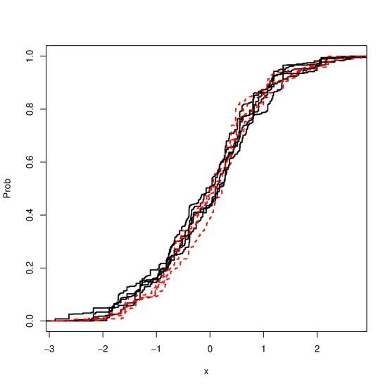
(a) $\mathbf{X}\sim N(0,1)$ and $\mathbf{Y}\sim N(0,1)$

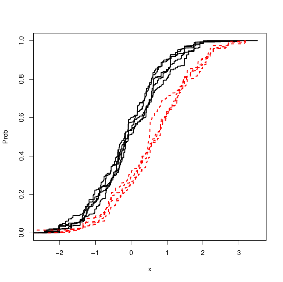
(b) $\mathbf{X}\sim N(0,1)$ and $\mathbf{Y}\sim N(1,1)$

Figure 1: The solid lines represent sample paths of the posterior Dirichlet process given the first sample and the dashed lines represent sample paths of the posterior Dirichlet process given the second sample.

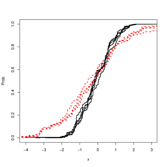
(a) $\mathbf{X}\sim N(0,1)$ and $\mathbf{Y}\sim N(0,2)$

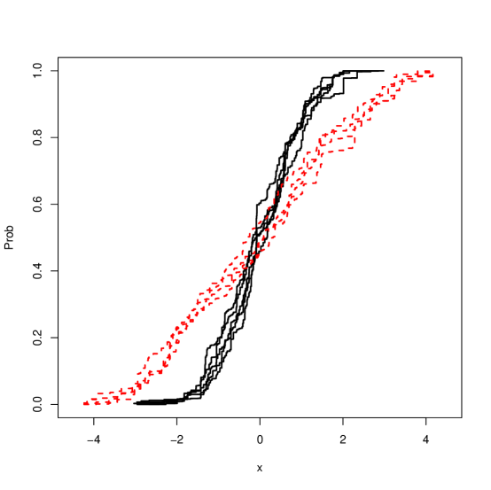
(b) $\mathbf{X}\sim N(0,1)$ and $\mathbf{Y}\sim 0.5N(-2,1)+0.5N(2,1)$

Figure 2: The solid lines represent sample paths of the posterior Dirichlet process given the first sample and the dashed lines represent sample paths of the posterior Dirichlet process given the second sample.

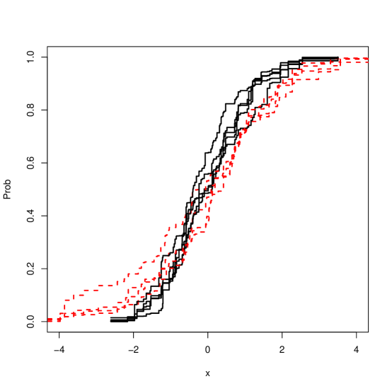
(a) $\mathbf{X}\sim N(0,1)$ and $\mathbf{Y}\sim t_{3}$

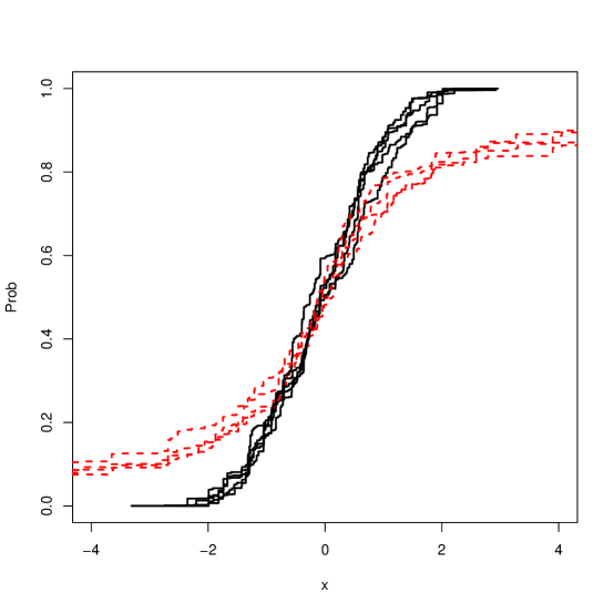
(b) $\mathbf{X}\sim N(0,1)$ and $\mathbf{Y}\sim t_{0.5}$

Figure 3: The solid lines represent sample paths of the posterior Dirichlet process given the first sample and the dashed lines represent sample paths of the posterior Dirichlet process given the second sample.

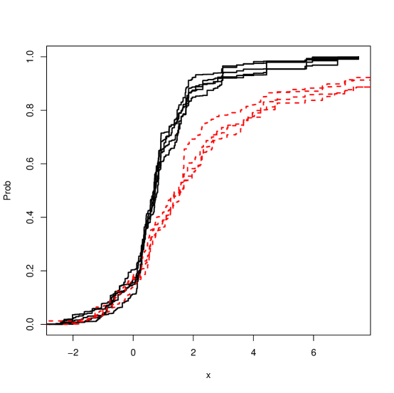
(a) $\log\mathbf{X}\sim N(0,1)$ and $\log\mathbf{Y}\sim N(1,1)$

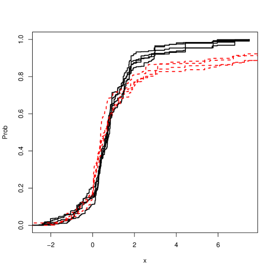
(b) $\log\mathbf{X}\sim N(0,1)$ and $\log\mathbf{Y}\sim N(0,2)$

Figure 4: The solid lines represent sample paths of the posterior Dirichlet process given the first sample and the dashed lines represent sample paths of the posterior Dirichlet process given the second sample.

Example 2. In this example, we study the performance of the proposed test as the sample size increases. We consider samples from the distributions given in Example 1, cases 1 and 2. The results are summarized in Table 2 and Table 3.

Table 2: Example 2: $\mathbf{X}\sim N(0,1)$ and $\mathbf{Y}\sim N(0,1)$.

Samples	$d$: Bayesian	U	p-value: K-S	p-value: Wilcoxon
$m_{1}=m_{2}=5$	0.50	0.69	0.8730	0.4206
$m_{1}=m_{2}=10$	0.41	0.56	0.7869	0.7959
$m_{1}=m_{2}=15$	0.33	0.48	0.9383	0.8381
$m_{1}=m_{2}=20$	0.31	0.42	0.5713	0.5683
$m_{1}=m_{2}=30$	0.23	0.36	0.3929	0.2301
$m_{1}=m_{2}=50$	0.14	0.28	0.7166	0.5192
$m_{1}=m_{2}=100$	0.15	0.20	0.5806	0.3958
$m_{1}=m_{2}=200$	0.12	0.16	0.5441	0.7598

Table 3: Example 2: $\mathbf{X}\sim N(0,1)$ and $\mathbf{Y}\sim N(1,1)$

Samples	$d$: Bayesian	U	p-value: K-S	p-value: Wilcoxon
$m_{1}=m_{2}=5$	0.72	0.70	0.0794	0.0317
$m_{1}=m_{2}=10$	0.73	0.56	0.0123	0.0005
$m_{1}=m_{2}=15$	0.61	0.47	0.0077	0.0010
$m_{1}=m_{2}=20$	0.53	0.42	0.00397	0.0132
$m_{1}=m_{2}=30$	0.52	0.36	0.0000	0.0000
$m_{1}=m_{2}=50$	0.50	0.28	0.0000	0.0000
$m_{1}=m_{2}=100$	0.46	0.20	0.0000	0.0000
$m_{1}=m_{2}=200$	0.39	0.16	0.0000	0.0000

It follows from Table 2 that, in all cases, the null hypothesis is not rejected. On the other hand, from Table 3, the null hypothesis is rejected. In both scenarios, the results are consistent with that obtained by the frequentist tests. Thus, the proposed test works even with sample sizes as small as 5. The power of the proposed test is examined in the next section.

5 Power Comparison

In this section, we empirically compare the power of the proposed test with the (standard) Kolmogorov-Smirnov test and the Wilcoxon test. We consider the following cases:

1. $\mathbf{X}\sim N(0,1)$ and $\mathbf{Y}\sim N(1,1)$

2. $\mathbf{X}\sim N(0,1)$ and $\mathbf{Y}\sim N(0,2)$

3. $\mathbf{X}\sim N(0,1)$ and $\mathbf{Y}\sim 0.5N(-2,1)+0.5N(2,1)$

4. $\mathbf{X}\sim N(0,1)$ and $\mathbf{Y}\sim t_{0.5}$

5. $\mathbf{X}\sim\text{Exponential}(1)$ and $\mathbf{Y}\sim\text{Exponential}(2)$. [$F_{X}(x)=1-e^{-x}$ and $F_{Y}(y)=1-e^{-2y}$]

The power of each test is estimated by calculating the proportion of rejecting the null hypothesis out of 1000 samples when the two sampling distributions are different (i.e. $F\neq G$). We consider several sample sizes. The simulation results are summarized in Table 4 to Table 8. The results in the tables indicate that the power of the proposed test is always greater than the power of the Kolmogorov-Smirnov test. On the other hand, as pointed out in Section 4, Wilcoxon test assumes that one of the samples must be a shifted version of the other. In practice, such assumption is not known a priori. Thus, Wilcoxon test is only useful for Case 1 and Case 5. Even in these two cases, the proposed test is as efficient as the Wilcoxon test. See Table 4 and Table 8.

Table 4: Power comparison from $\mathbf{X}\sim N(0,1)$ and $\mathbf{Y}\sim N(1,1)$.

Samples	Bayesian	K-S	Wilcoxon
$m_{1}=m_{2}=5$	0.343	0.075	0.235
$m_{1}=m_{2}=10$	0.480	0.218	0.484
$m_{1}=m_{2}=15$	0.670	0.533	0.711
$m_{1}=m_{2}=20$	0.840	0.724	0.855
$m_{1}=m_{2}=30$	0.948	0.885	0.963
$m_{1}=m_{2}=50$	0.995	0.982	0.995
$m_{1}=m_{2}=100$	1	1	1
$m_{1}=m_{2}=200$	1	1	1

Table 5: Power comparison from $\mathbf{X}\sim N(0,1)$ and $\mathbf{Y}\sim N(0,2)$.

Samples	Bayesian	K-S	Wilcoxon
$m_{1}=m_{2}=5$	0.123	0.01	0.049
$m_{1}=m_{2}=10$	0.108	0.022	0.049
$m_{1}=m_{2}=15$	0.125	0.067	0.048
$m_{1}=m_{2}=20$	0.217	0.124	0.054
$m_{1}=m_{2}=30$	0.332	0.184	0.059
$m_{1}=m_{2}=50$	0.667	0.371	0.051
$m_{1}=m_{2}=100$	0.979	0.800	0.060
$m_{1}=m_{2}=200$	1	0.997	0.059

Table 6: Power comparison from $\mathbf{X}\sim N(0,1)$ and $\mathbf{Y}\sim 0.5N(-2,1)+0.5N(2,1)$.

Samples	Bayesian	K-S	Wilcoxon
$m_{1}=m_{2}=5$	0.176	0.025	0.056
$m_{1}=m_{2}=10$	0.303	0.075	0.065
$m_{1}=m_{2}=15$	0.545	0.277	0.079
$m_{1}=m_{2}=20$	0.784	0.472	0.074
$m_{1}=m_{2}=30$	0.949	0.762	0.075
$m_{1}=m_{2}=50$	1	0.982	0.076
$m_{1}=m_{2}=100$	1	1	0.066
$m_{1}=m_{2}=200$	1	1	0.075

Table 7: Power comparison from $\mathbf{X}\sim N(0,1)$ and $\mathbf{Y}\sim t_{0.5}$.

Samples	Bayesian	K-S	Wilcoxon
$m_{1}=m_{2}=5$	0.109	0.015	0.046
$m_{1}=m_{2}=10$	0.107	0.028	0.057
$m_{1}=m_{2}=15$	0.135	0.061	0.057
$m_{1}=m_{2}=20$	0.226	0.110	0.058
$m_{1}=m_{2}=30$	0.338	0.187	0.059
$m_{1}=m_{2}=50$	0.762	0.491	0.049
$m_{1}=m_{2}=100$	1	0.943	0.061
$m_{1}=m_{2}=200$	1	1	0.051

Table 8: Power comparison from $\mathbf{X}\sim\text{Exponential}(1)$ and $\mathbf{Y}\sim\text{Exponential}(2)$.

Samples	Bayesian	K-S	Wilcoxon
$m_{1}=m_{2}=5$	0.173	0.026	0.100
$m_{1}=m_{2}=10$	0.202	0.069	0.209
$m_{1}=m_{2}=15$	0.315	0.226	0.337
$m_{1}=m_{2}=20$	0.446	0.321	0.444
$m_{1}=m_{2}=30$	0.589	0.484	0.620
$m_{1}=m_{2}=50$	0.847	0.746	0.832
$m_{1}=m_{2}=100$	0.994	0.961	0.991
$m_{1}=m_{2}=200$	1	1	1

6 Additional Properties

In this section, we discuss some additional properties of the proposed method for the goodness-of-fit test. The next lemma shows that, under the null hypothesis, the Kolmogorov distance between posterior distributions given the data converges to zero as sample sizes get large.

Lemma 1.

If $P^{*}_{m_{1}}$ is the posterior distribution of the Dirichlet process given the first and $Q^{*}_{m_{2}}$ is the posterior distribution of the Dirichlet process given the second sample. Then, under $\mathcal{H}_{0}$, we have

$$d(P^{*}_{m_{1}},Q^{*}_{m_{2}})\to 0,$$

as $m_{1},m_{2}\to\infty$. Recall, $m_{i}$ represents the sample size of the sample $i$, $i=1,2$.

Proof.

It follows from the triangle inequality that

$$d\left(P^{*}_{m_{1}},Q^{*}_{m_{2}}\right) \leq d\left(P^{*}_{m_{1}},H^{*}_{m_{1}}\right)+d\left(Q^{*}_{m_{2}},H^{*}_{m_{1}}\right)$$ (6.1)

$$\leq d\left(P^{*}_{m_{1}},H^{*}_{m_{1}}\right)+d\left(Q^{*}_{m_{2}},H^{*}_{m_{2}}\right)+d\left(H^{*}_{m_{1}},H^{*}_{m_{2}}\right),$$

where $H^{*}_{m_{i}}$ is defined in (2.1) for any continuous base measure $H$, $i=1,2$. The proof of the lemma is complete since, under $\mathcal{H}_{0}$, the right hand side of the inequality (6.1) converges to zero as $m_{1},m_{2}\to\infty$ (Ferguson, 1973; Goshal, 2010; Al Labadi and Zarepour, 2013b). ∎

Next, we show empirically that the proposed technique of goodness-of-fit test is robust against prior specification the Dirichlet process’ parameters (i.e., the concentration parameter and the base measure). To this end, we have repeated Example 1 in Section 4 with two additional cases. In the first case, we take $H$ to be the uniform distribution on $[0,1]$ and $a=1$. In the second case, we take $H$ to be the standard normal distribution and $a=50$. The results are reported in Table 9. It follows clearly from Table 9 that the conclusions drawn in Example 1 are not affected by changing either $H$ or $a$. Specifically, fixing $a$ and changing $H$, will not change either the distance or $U$. This is due to the fact that the distance is measured between two Dirichlet processes, which only depends on the cumulative weights of each Dirichlet process. Thus, the distance and $U$ are independent from $H$. On the other hand, fixing $H$ and changing $a$ changes both the distance and $U$. If $a$ is increased (decreased), then the both distance and $U$ are decreased (increased) in such way that conclusions are not affected and remain the same.

Table 9: Robustness of the Bayesian nonparametric test against changing the parameters of the Dirichlet process

Samples	$d:H=N(0,1),a=1$	$d:H=U[0,1],a=1$	$d:H=N(0,1),a=50$
1	0.15	0.15	0.12
2	0.42	0.42	0.30
3	0.26	0.26	0.19
4	0.44	0.44	0.30
5	0.19	0.19	0.15
6	0.31	0.31	0.21
7	0.42	0.42	0.29
8	0.26	0.26	0.19
$U$	0.20	0.20	0.18

7 Concluding Remarks

A method based on the Kolmogorov distance and approximate samples from the Dirichlet process is proposed to asses the equality of two unknown distributions. The new approach is simple and flexible such that it can be applied to any two-sample problem with any sample size. As shown in the power study, the proposed test has distinctly higher power than the power of several popular tests in many cases. In particular, the proposed test dominates the standard Kolmogorov-Smirnov test in all the cases examined in the present paper. On the other hand, unlike most frequentist tests, the proposed test is not based on computing p-values. The main concern about using p-values in testing statistical hypothesis is that they overestimate the evidence against the null hypothesis (Masson, 2011; Sawrtz, 1999; Wagenmakers, 2007). For instance, see Table 1.

The current study may lead to further research directions. For instance, it would be interesting to study the effect of selecting other distances such as the Wasserstein (or Kantorovich) distance and the Kullback-Leibler distance on the proposed approach. Another important extension is the generalization of the approach to construct a goodness-of-fit test for multivariate distributions. In principle, there is no need to change the methodology. However, the calculation of the distance requires amendment in this case. Extending the approach to multivariate distributions will bypass the distribution-free problem for the tests that rely on the empirical distribution function. Finally, similar to the frequentist’s Kolmogorov-Smirnov test, it is possible to construct a test based on the fact that the two independent processes $\sqrt{m_{1}}\left(P^{*}_{m_{1}}-H^{*}_{m_{1}}\right)$ and $\sqrt{m_{2}}\left(P^{*}_{m_{2}}-H^{*}_{m_{2}}\right)$ converge jointly in distribution to the two independent Brownian bridges $B_{F}$ and $B_{G}$, where $F$ and $G$ are the “true” distributions generating the data. Recall that, for a collection of Borel sets $\mathscr{S}$ in $\mathbb{R}$, a Gaussian process $\left\{B_{F}(S):S\in\mathscr{S}\right\}$ is called a Brownian bridge with parameter measure $F$ if ${E}\left[B_{F}(S)\right]=0$ for any $S\in\mathscr{S}$ and ${Cov}\left(B_{F}(S_{1}),B_{F}(S_{2})\right)=F(S_{1}\cap S_{2})-F(S_{1})F(S_{2})$ for any $S_{1},S_{2}\in\mathscr{S}$ (Kim and Bickel, 2003). We leave this direction for future work.

Appendix

Table 10: Values of $U$ (upper bound of the 95% prediction interval for the prior distance $d_{0}$).

	$m_{1}$
$m_{2}$	1	2	3	4	5	6	7	8	9	10	11	12	13	14	15	16	17	18	19	20
1	0.93
2	0.90	0.86
3	0.87	0.82	0.79
4	0.87	0.80	0.78	0.74
5	0.84	0.79	0.74	0.72	0.69
6	0.84	0.78	0.74	0.71	0.67	0.66
7	0.82	0.78	0.72	0.69	0.67	0.64	0.63
8	0.82	0.75	0.69	0.68	0.64	0.64	0.62	0.60
9	0.79	0.76	0.71	0.69	0.64	0.61	0.61	0.60	0.58
10	0.81	0.76	0.71	0.68	0.62	0.60	0.58	0.58	0.58	0.55
11	0.83	0.74	0.67	0.63	0.61	0.59	0.58	0.57	0.55	0.54	0.52
12	0.79	0.73	0.66	0.67	0.63	0.58	0.58	0.56	0.55	0.54	0.52	0.52
13	0.80	0.72	0.67	0.64	0.59	0.58	0.55	0.56	0.53	0.54	0.51	0.51	0.50
14	0.79	0.73	0.66	0.64	0.60	0.57	0.57	0.54	0.53	0.52	0.51	0.51	0.50	0.49
15	0.79	0.71	0.67	0.62	0.60	0.57	0.55	0.54	0.51	0.51	0.50	0.50	0.50	0.47	0.47
16	0.79	0.70	0.65	0.61	0.59	0.59	0.56	0.53	0.53	0.52	0.51	0.51	0.49	0.47	0.46	0.45
17	0.79	0.72	0.67	0.63	0.59	0.56	0.56	0.53	0.52	0.50	0.49	0.49	0.47	0.47	0.46	0.45	0.45
18	0.80	0.72	0.66	0.62	0.60	0.58	0.55	0.53	0.52	0.51	0.48	0.47	0.47	0.48	0.45	0.45	0.44	0.44
19	0.79	0.70	0.65	0.63	0.58	0.57	0.53	0.54	0.51	0.49	0.49	0.47	0.46	0.46	0.44	0.45	0.45	0.42	0.44
20	0.79	0.73	0.65	0.62	0.59	0.57	0.54	0.51	0.49	0.49	0.49	0.47	0.46	0.44	0.44	0.45	0.43	0.43	0.42	0.42

References

- [1] Al Labadi, L., and Zarepour, M. (2013a), ‘A Bayesian nonparametric goodness of fit test for right censored data based on approximate samples from the beta-Stacy process’, Canadian Journal of Statistics, 41, 3, 466–487.
- [2] Al Labadi, L., and Zarepour, M. (2013b), ‘On asymptotic properties and almost sure approximation of the normalized inverse-Gaussian process’, Bayesian Analysis, 8, 553–568.
- [3] Al Labadi, L., and Zarepour, M. (2014a), ‘On simulations from the two-parameter Poisson-Dirichlet process and the normalized inverse-Gaussian process’, Sankhya A, 76,158–176.
- [4] Al Labadi, L., and Zarepour, M. (2014b), ‘Goodness of fit tests based on the distance betweenthe Dirichlet process and its base measure’, To appear in Journal of Nonparametric Statistics, DOI: 10.1080/10485252.2013.856431.
- [5] Berger, J.O., and Guglielmi, A. (2001), ‘Bayesian testing of a parametric model versus nonparametric alternatives’, Journal of the American Statistical Association, 96, 174–184.
- [6] Blackwell, D., and MacQueen, J.B. (1973), ‘Ferguson distributions via Polya urn schemes’, Annals of Statistics, 1, 353–355.
- [7] Bondesson, L. (1982), ‘On simulation from infinitely divisible distributions’, Advances in Applied Probability, 14, 885–869.
- [8] Borgwardt, K.M., and Ghahramani, Z. (2009), ‘Bayesian two-sample tests’. http://arxiv.org/abs/0906.4032.
- [9] Carota, C., and Parmigiani, G. (1996), ‘On Bayes factors for nonparametric alternatives’, in Bayesian Statistics 5, ed. J.M. Bernardo, J.O. Berger, A.P. Dawid, and A.F.M. Smith, London, 1996: Oxford University Press, 508–511.
- [10] Cifarelli, D.M., and Regazzini, E. (1990), ‘Distribution functions of means of a Dirichlet process’, Annals of Statistics, 18, 429–442.
- [11] Chen, Y., and Hanson, T. (2014), ‘Bayesian nonparametric k-sample tests for censored and uncensored data’, Computational Statistics and Data Analysis, 71, 335–346.
- [12] Ferguson, T.S. (1973), ‘A Bayesian analysis of some nonparametric problems’, Annals of Statistics, 1, 209–230.
- [13] Ferguson, T.S., and Klass, M.J. (1972), ‘A representation of independent increment processes without Gaussian components’, Annals of Mathematical Statistics, 1, 209–230.
- [14] Florens, J.P., Richard, J.F., and Rolin, J.M. (1996), ‘Bayesian encompassing specification tests of a parametric model against a nonparametric alternative’, Technical Report 9608, Universitsé Catholique de Louvain, Institut de statistique.
- [15] Ghosal, S. (2010), ‘The Dirichlet process, related priors and posterior asymptotics’, in Bayesian Nonparametrics, ed. N.L Hjort, C.C. Holmes, P. Müller and S. Walker, Cambridge: Cambridge University Press, 35–79.
- [16] Ghosh, J.K., and Ramamoorthi, R.V. (2003), Bayesian Nonparametrics, New York: Springer.
- [17] Hsieh, P. (2011), ‘A nonparametric assessment of model adequacy based on Kullback-Leibler divergence’, Statistics and Computing, 23, 149–162.
- [18] Holmes, C. C., Caron, F., Griffin, J. E., and Stephens, D. A. (2015), ‘Two-sample Bayesian nonparametric hypothesis testing’. Bayesian Analysis2, 297-320.
- [19] Ishwaran, H., James, L.F., and Zarepour, M. (2009), ‘An alternative to out of bootstrap’, Journal of Statistical Planning and Inference, 39, 788–801.
- [20] James, L.F. (2005), ‘Functionals of Dirichlet processes, the Cifarelli-Regazzini identity and beta-gamma processes’, Annals of Statistics, 33, 647–660.
- [21] James, L.F. (2006), ‘Poisson calculus for spatial neutral to the right processes’, Annals of Statistics, 34, 416–440.
- [22] James, L.F (2008), ‘Large sample asymptotics for the two-parameter Poisson- Dirichlet process’, in Pushing the Limits of Contemporary Statistics: Contributions in Honor of Jayanta K. Ghosh, ed. B. Clarke and S. Ghosal, Ohio: Institute of Mathematical Statistics, 187–199.
- [23] James, L.F., Lijoi, A., and Prünster, I. (2006), ‘Conjugacy as a distinctive feature of the Dirichlet process’, Scandinavian Journal of Statistics, 33, 105–120.
- [24] Kim, N., and Bickel, P. (2003), ‘The limit distribution of a test statistic for bivariate normality’, Statistica Sinica, 13, 327–349.
- [25] Lavine, M. (1992), ‘Some aspects of Polya tree distributions for statistical modelling’, Annals of Statistics, 20, 1222–1235.
- [26] Lijoi, A., and Regazzini, E. (2004), ‘Means of a Dirichlet process and multiple hypergeometric functions’, Annals of probability, 32, 1469–1495.
- [27] Lo , A.Y. (1987), ‘A large sample study of the Bayesian bootstrap’, Annals of Statistics, 15, 360–375.
- [28] Ma, L., and Wong, W.H (2011), ‘Coupling optional pólya trees and the two sample problem’, Journal of the American Statistical Association, 106, 1553–1565.
- [29] McVinish, R., Rousseau, J., and Mengersen, K. (2009), ‘Bayesian goodness of fit testing with mixtures of triangular distributions’, Scandivavian Journal of Statistics, 36, 337–354.
- [30] Muliere, P., and Tardella, L. (1998), ‘Approximating distributions of random functionals of Ferguson-Dirichlet prior’, Canadian Journal of Statistics, 26, 283–297.
- [31] Regazzini, E., Guglielmi, A., and Di Nunno, G. (2002), ‘Theory and numerical analysis for exact distribution of functionals of a Dirichlet process’, Annals of Statistics, 30, 1376–1411.
- [32] Sethuraman, J. (1994), ‘A constructive definition of Dirichlet priors’, Statistica Sinica, 4, 639–650.
- [33] Swartz, T.B. (1999), ‘Nonparametric goodness-of-fit’, Communications in Statistics: Theory and Methods, 28, 2821–2841.
- [34] Viele, K., (2000), ‘Evaluating fit using Dirichlet processes’, Technical Report 384, University of Kentucky, Dept. of Statistics.
- [35] Wolpert, R.L., and Ickstadt, K., (1998), ‘Simulation of Lévy random fields’, in Practical Nonparametric and Semiparametric Bayesian Statistics, ed. : D. Day, P. Nuller, and D. Sinha, Springer, 227–242.
- [36] Zarepour, M., and Al Labadi, L. (2012), ‘On a rapid simulation of the Dirichlet process’, Statistics and Probability Letters, 82, 916–924.