Images from the Mind: BCI image evolution based on RSVP of polygon primitives

Abstract

This paper provides a proof of concept for an EEG-based reconstruction of a visual image which is on a user’s mind. Our approach is based on the Rapid Serial Visual Presentation (RSVP) of polygon primitives and Brain-Computer Interface (BCI) technology. The presentation of polygons that contribute to build a target image (because they match the shape and/or color of the target) trigger attention-related EEG patterns. Accordingly, these target primitives can be determined using BCI classification of Event-Related Potentials (ERPs). They are then accumulated in the display until a satisfactory reconstruction is reached. Selection steps have an average classification accuracy of $75\%$. $25\%$ of the images could be reconstructed completely, while more than $65\%$ of the available visual details could be captured on average. Most of the misclassifications were not misinterpretations of the BCI concerning users’ intent; rather, users tried to select polygons that were different than what was intended by the experimenters. Open problems and alternatives to develop a practical BCI-based image reconstruction application are discussed.

1 Introduction

We introduce a Brain-Computer Interface (BCI) application based on Rapid Serial Visual Presentation (RSVP) of polygon primitives for image reconstruction. Our paradigm relies on the decomposition of a collection of images (figure 1) into a set of approximate constituent parts (polygon primitives). These primitives are presented to the experimental subjects in bursts. Event Related Potentials (ERPs) associated with the oddball paradigm [1, 2] are used as EEG correlates to detect those pieces that contribute to the reconstruction of the target image (which is on the user’s mind) in an incremental fashion. The operational basis (RSVP) has already been employed for BCI-based gaze-independent spellers [3, 4] and an Icon Messenger [5]. The results presented in this paper invite us to be optimistic about this new paradigm for BCI image reconstruction. More experiments should be carried out to expand the design outside the chosen collection of images, ideally moving towards a free-painting device. Some ideas are proposed based on the outcome of the current work. The experiments also suggest ways to increase the reliability, speed, and accuracy of the current framework.

Our work draws from recent advances in Cortically-Coupled Computer Vision (C3Vision) [6, 7, 8] where human vision is enhanced through an efficient data mining of EEG patterns while stimuli are presented. Such an approach has shown to boost the search for target images, and how to speed up the localization of salient details from within a large image [9, 10]. Even further improvement can be achieved with a closed loop philosophy in which human vision and EEG are not only coupled, but engage in a cycle where the artificial intelligence behind the EEG-based classifiers offers feedback in real time [11, 12]. These seminal studies provide interesting insights about the capabilities of such BCIs and suggest that the limits of our own design could be pushed further.

In [13] we find an early approach closer to the line of research that we pursue. Physiological states – including EEG and indicators such as ventilation, heart rate, and others – are correlated to ‘positive’ and ‘negative’ feelings elicited by visual stimuli. The ability to prompt positive reactions is then used as fitness functions for new, randomly generated images that evolve by means of a genetic algorithm. The decisions based on these cues are compared offline to the deliberate choices made by the experimental subjects who should decide what images were more artsy. These physiological correlates predict up to $61\%$ of the subjects’ choices. It is more complicated to assess the global goal of this research – i.e. evolving art.

The main drawback of this paradigm is the extended exposure time needed to gather the relevant physiological data. Subjects are exposed to pictures for one second so that neural correlates of mood can be recorded. This stretches a single generation of the genetic algorithm to $12$ minutes. Because of this large exposure, it is likely that only coarse features of a picture are relevant for selection. This might be a problem for practical applications, if we wanted to direct the evolution towards detailed visual features. Additionally, the only selective pressures are “positive” feelings elicited by the drawings, for which it is difficult to quantify a progress: Does the last image render more positive feelings than the original one? How long can we advance in positiveness before the physiological correlates saturate? These thorny details, rather than flaws in the original design, reveal the difficulty of the task under consideration.

While the authors of [13] intended to explore the undetermined space of art and feelings evoked by drawings, Shamlo and Makeig [14] sketch a procedure to evolve towards a definite target image. Bursts of randomly generated drawings are presented to the subjects, whose EEGs are recorded. A burst might or might not contain a target image that resembles “two eyes”. The subject presses a button after each burst to indicate if the target has been consciously spotted out. EEG patterns are extracted that correlate with the presence of the target image during a burst. The authors focus on processing the data during a posterior offline analysis. Using ten fold cross-validation on data from a single trial, very high accuracy is obtained (up to $0.98$ area under ROC curve of correctly classified target pictures).

Encouraged by these good results, and in the spirit of C3Vision, the authors propose to use their BCI paradigm to bypass the slow feedback that subjects have to provide manually nowadays. One straightforward application suggested is to use this EEG activity to evolve images. Currently existing software [15], accepts user-provided images and attempts to evolve them towards a desired target picture. Random mutations and crossover are applied to the original seed to generate new drawings. In the standard approach, the user manually chooses among the new candidates that fall closer to an arbitrary goal (e.g. “two eyes” as in [14]). This manual procedure is cumbersome. Using EEG correlates to identify what images should be fed to the algorithm could speed up the evolutionary process. Unfortunately, such interesting possibility is only suggested in [14] based on the exceptional performance of the EEG-driven classification task. Actual experiments should be implemented to test the complete BCI–evolutionary-algorithm loop. When this is done, it will be possible to address an important aspect of the BCI design. The performance reported in [14] refers to the identification of target images within bursts that the experimental subject manually identified as containing a target. The high accuracy of this manual selection ($94\%$ correct classifications) indicates that the task (the identification of a broad feature such as “two eyes”) might be simple enough. It is an open question about how accurate the procedure will be once the tasks become harder, e.g. if we would attempt to evolve more detailed visual structures.

The P300-Brain Painting BCI [16, 17, 18] inspired by the early P300-Speller BCIs [19] is the device closer to ours in goals and performance. Using the oddball paradigm, colors, shapes, and a variety of tools are selected from a matrix of highlighted rows and columns. The selected operators modify an existing canvas in a similar way that a mouse interface would do. In [18] this BCI was evaluated in healthy and ALS patients finding, for certain design specifications, performances comparable to those of the equivalent matrix speller. The insights from these works – in terms of speed and accuracy – are complicated to translate to ours due to the important differences in implementation. We investigate two different – albeit similar in purpose – designs, and this will complicate the comparison between BCIs as discussed below.

The painting tools available in [18] are rather scarce: two shapes (square and circle), eight colors, and four sizes. Despite this potential limitation, the subjects can produce quite complex paintings (figure 3 in [18]). If we wanted to incorporate more shapes or colors, we might face an important limitation since the number of painting tools must fit in the symbol matrix: a larger matrix (more tools) will translate in lower selection accuracy. As the authors point out, this problem affects the movement of the mouse cursor too: only eight directions are allowed along which the cursor moves one single unit at a time. It is suggested to use sensorimotor rhythms to control a mouse pointer over the canvas. That would release space in the symbol matrix for other needs. Despite these minor issues, the BCI in [18] must be regarded as an important breakthrough for BCI-painting.

The paradigm explored in [13] relies on physiological signals. This slows down the interface drastically, as tens of seconds are necessary to collect reliable data. But the approach in [14] and others [11, 12] set an interesting precedent for our BCI given the high rate at which stimuli are presented (up to $12$ Hz). We chose more conservative rates (around $3$ Hz) for the proof of concept introduced here. Another crucial difference between most examples in the literature and ours is that we proceed bottom-up to reconstruct a set of images: our stimuli are polygon primitives that might resemble smaller details of a target drawing, which allows for a finer grained reconstruction than those in [13, 14]. In these studies, each stimulus is a whole picture and targets are based on broader features such as the existence of two eyes. This would be important, if we wanted to extrapolate the technical setup (mainly the stimulus rate) to our design. Furthermore experiments actual image reconstructions were undertaken, thus we offer the first serious test of this novel and promising BCI paradigm.

The paper is organized as follows: In section 2 the proposed BCI is described along with the experimental and data analysis details. In section 3 the results are summarized. We close with a discussion of these results (in comparison with the existing literature) in section 4, where future lines of research are proposed together with possible improvements and alternatives to the current design. Appendix A includes a description of the choices made regarding the preprocessing of the images and the experimental setup. This is compared to similar BCI schemes that inspired the research. Appendix B analyzes in detail an anomaly found in some image reconstructions.

2 Methods

2.1 Participants

Ten participants (five women and five men, ages ranging from early twenties to early thirties) took part in the experiment on a voluntary, non rewarded basis. One of the subjects was associated to the BCI research group. This subject and two others had previous experiences with BCI experiments. The rest of the subjects were naïve with respect to BCI technologies. All of them had normal or corrected to normal vision and did not report any health issues during the experiment.

2.2 Apparatus

EEG was recorded at 1000 Hz using BrainAmp amplifiers and an ActiCap active electrode system with $63$ channels (Brain Products, Munich, Germany). The electrodes used were Fp1,2, AF3,4,7,8, Fz, F1-10, FCz, FC1-6, FT7,8, Cz, C1-6, T7,8, CPz, CP1-6, TP7,8, Pz, P1-10, POz, PO3,4,7,8, Oz, O1,2. All electrodes were referenced to the left mastoid using a forehead ground. For offline analyses, electrodes were re-referenced to linked mastoids. All the impedances were kept below $10\>k\Omega$.

Stimuli were presented on a $24$” TFT screen with a refresh rate of $60\>Hz$ and a resolution of $1920\times 1200 \>px^{2}$. The experiment was implemented in Python using the open-source BCI framework Pyff [20] with Pygame [21] and Vision-Egg [22]. Data analysis and classification were performed with MATLAB (The MatlabWorks, Natick, MA, USA) using an in-house BCI toolbox (www.bbci.de/toolbox).

2.3 Design and procedure

The design of the experiment includes a pre-processing of the images to extract the primitives that are shown during RSVP bursts. Important choices regarding stimulus presentation were also made. Because we explore a novel paradigm, almost any design feature is open to debate. In the following, we report the actual choices made for the experiment. For an introduction and discussion of the other possibilities the reader is referred to appendix A.

2.3.1 Preprocessing of target images

The nine drawings of fruits and vegetables collected in figure 1 were chosen as potential targets for reconstruction from the revised Snodgrass and Vanderwart’s object database [23]. They are easily recognizable, have bright, plain colors, and combine basic shapes with some minor details – such as the stalk of a cherry – that could act as landmarks during a reconstruction task. They are always displayed upon a blank background.

Figure 1: Images selected as BCI reconstruction targets. The chosen images comprise very basic and recognizable shapes with bright colors. Besides, some of the drawings present relatively small details that become important as the reconstruction advances. We also show the polygon decompositions obtained for each image.

Similar to the role played by characters in RSVP spellers [3, 4], we need nuclear units that constitute stimuli during the bursts of our BCI paradigm. These stimuli must be able to reconstruct the target images as they accumulate in the screen. We submitted the chosen images to a preprocessing step during which a genetic algorithm [24] extracted a series of primitives (polygons) that approximated the drawings up to a satisfactory degree (final product shown in figure 1). We refer to these primitives throughout the text as the polygon decomposition of each of the targets. A brief description of the genetic algorithm is found in appendix A.1. The actual code that we used and the values of different parameters chosen for our implementation can be found in a public repository [25].

The resulting decompositions contain between $4$ and $10$ polygons (with $6.7$ on average) depending on the target drawing. We restricted polygons to have between $3$ and $7$ vertices and solid colors – i.e. no transparency was allowed. Polygons are overlaid on a blank background and on each other, thus their order matters for the reconstruction task.

The fitness function used as a selection criterion by the genetic algorithm (see appendix A.1) is a pixel-by-pixel distance between an image and its polygon decomposition. By computing the fitness drop of a decomposition when one polygon is removed, we have a measure of the impact of each polygon in the final reconstruction. We dub this measure visual information and report it as a percentage. When running the BCI experiments we only used polygons with a visual information higher than $3\%$ ($15\%$ during the calibration phase – see sec. 2.3.2). On average, the polygons eventually selected for the experiments bore a visual information of $13.5\%$ with a standard deviation of $13.4\%$.

This visual information also allows us to rank the polygons within a decomposition according to their importance in the reconstruction. We used this ranking to select what target polygons are displayed in the initial bursts of the reconstruction, and we moved towards less informative polygons as the reconstruction proceeded, as explained in section 2.3.2.

Finally, the oddball paradigm targets are displayed among allegedly neutral non-target stimuli. Whenever a picture was selected for reconstruction, the polygons in its decomposition were considered target primitives. The polygons from the decomposition of all non-target images were held in a pool from which non-target primitives were drawn at the beginning of each burst (see appendix A.1 for discussion).

2.3.2 Experimental setup

The experiment consisted of a calibration phase and a reconstruction phase, schematically depicted in figure 2. In either phase, a drawing from figure 1 was selected as a target and displayed for $5$ seconds prior to each burst. A burst consisted of the rapid presentation of polygons that included target and non-target stimuli – i.e. primitives from the decomposition of the target and non-target images respectively. For each burst, $5$ non-target polygons were selected for display together with the (one) corresponding target polygon.

Figure 2: Schematic representation of bursts during different phases of the experiment. a Calibration phase: Bursts of polygons are presented to the subjects with no feedback between bursts. A target picture is randomly chosen for each burst. Stimuli in this phase are restricted to polygons bearing more than $15\%$ visual information to ensure that ERPs are reliably elicited and measured. b Reconstruction phase: A target picture is chosen and remains target for several bursts until its reconstruction is completed. Each burst presents new target polygons upon the background where previous target primitives accumulate, thus implementing the image reconstruction. After each burst a feedback is provided showing the correct polygon and the polygon selected by the classifier. Despite the classification result, the correct polygon is always kept in successive bursts so that the reconstruction can proceed. An example of the reconstruction implemented is shown in [26].

A burst involves a number of blocks that may be different for the calibration and reconstruction phases. Each block consists of the display of all $6$ polygons in a shuffled order. Each polygon is shown just once per block. The only constraint to the random order within a burst is that no primitive may appear twice in immediate succession. Because a burst is a series of blocks, this restriction only affects the randomness of a block given the last stimulus of the previous block. The stimulus onset asynchrony (SOA) between successive polygons was $330 \>ms$: during $230\>ms$ the visual stimulus (the polygon) was shown and during the last $100 \>ms$ the corresponding polygon was substituted by a transparent rectangle – i.e. by a void stimulus.

Calibration phase: We restricted the visual stimuli to those polygons contributing more than $15\%$ visual information. By avoiding polygons that might not be reliably recognized as targets by the participant (due to little visual information), ERPs elicited by the target polygons were likely a valid signal to calibrate the classifier. Before each burst, a picture was selected as the target image and one random polygon from its decomposition (among those with a visual information above $15\%$) was selected as the target primitive. During this phase, a burst consisted of $4$ blocks for subjects VPmao, VPmap, and VPjam, and of $10$ blocks for any other subject. After each burst, a new target image was selected. The subjects were told that, following the display of a drawing, random polygons would be presented and one or more of them could resemble the drawing or some salient feature of it. They were not explicitly instructed to seek for these stimuli in an active way. They were requested to avoid abrupt facial movements, to avoid blinking and to relax the jaw. Approximately each $15$ minutes a self-paced pause was offered. During the calibration phase, there was no feedback provided to the participants.

Reconstruction phase: We considered all polygons from the decompositions that contributed more than $3\%$. For each subject, $15$ reconstructions were completed. After choosing one of the images for reconstruction, it was displayed for $5$ seconds. Then the first burst proceeded with the most informative polygon of the chosen image as target, together with $5$ non-targets drawn from the pool of polygons. Bursts during this phase consisted of $4$ blocks for subjects VPmai and VPmao, and $10$ for any other subject. During each burst of the reconstruction phase, the classifier would score the likelihood that each polygon had elicited an ERP, and at the end of the burst the primitive being most likely the target was determined, as explained in section 2.4. This primitive was displayed for $5$ seconds as a feedback alongside the correct target polygon. Then the original target picture under reconstruction was shown again for $5$ seconds. The next burst proceeded with the next most informative polygon as target and with $5$ new non-targets from the polygon pool. The correct stimuli from previous bursts were retained after they had been played out, so that the reconstruction could proceed. After a reconstruction was completed, a self-paced pause was offered. The instructions to the subjects were the same as during the calibration phase, except now subjects were told that the reconstruction would proceed until a fair, schematic rendering of the target image had been reached. A video of a successful reconstruction is available [26].

2.4 Data analysis

ERP analysis: EEG signals were lowpass filtered with a Chebyshev filter using a bandpass up to $40\>Hz$ and a stopband starting at $49\>Hz$, and then down-sampled to $100\>Hz$. Continuous signals were divided into epochs ranging from $-200\>ms$ to $1000\>ms$ relative to each stimulus onset. Baseline correction was performed on the pre-stimulus interval of $200\>ms$. Epochs containing strong eye movements were detected and rejected using the following criterion: Epochs in which the difference of the maximum and the minimum values in one of the channels F9, Fz, F10, AF3, and AF4 exceeded $70\>\mu V$ were rejected. Only those non-target epochs were used in which the three preceding and the three following symbols were also non-targets in order to avoid overlap from ERPs of preceding or successive targets. For the grand average the ERP curves were averaged across all trials and participants. To compare the ERP curves of two classes (target and non-target) signed $r^{2}$-values were calculated.

Classification of what polygons the subject attended to: We employed binary classifiers based on spatio-temporal features. We sought for discrimination between epochs related to targets vs. non-targets. As preprocessing, EEG signals were down-sampled to $100\>Hz$ by calculating the average for consecutive data points in non-overlapping stretches of $10\>ms$ each. Epochs with an excessive power in a broadband ($5-40\>Hz$) indicating, e.g. muscular artifacts, were rejected from the calibration data. The aim of the heuristic is to find five time intervals that have a stationary (target minus non-target difference) pattern and maximal $r^{2}$ differences. Occasionally the intervals determined by the heuristic were adjusted by the experimenter before starting the on-line runs (see appendix A.2). Features were calculated from $55$ channels (all except for Fp1,2, AF3,4, F9,10, FT7,8; which are the electrodes more exposed to facial movements) by averaging voltages within each of the five chosen time windows resulting in $55\times 5=275$ dimensional feature vectors. For classification, a linear discriminant analysis (LDA) with shrinkage of the covariance matrix [27] was trained on calibration data. A polygon was determined by averaging the classifier output for all displayed polygons across the $4$ or $10$ blocks of each burst and then by choosing the primitive that received the largest average output.

In order to investigate the rate/accuracy tradeoff, the classifier that was used online was also applied offline to the image reconstruction data. The polygon selection depended then on averages across the first n blocks, with $n=1,\dots,10$. For $n=10$ the full neural records are analyzed, so we obtain the same results as when operating the classifier online. For $n<10$, some of the data within each trial is discarded, so we are estimating the performance of the classifier if shorter neural activity records were available. We also computed the Information Transfer Rate per decision ($ITR_{d}$) – i.e. the number of bits involved in each classification – using:

$$ITR = log_{2}(N)+p_{c}\>log_{2}(p_{c})+$$ (1)

$$+(1-p_{c})\>log_{2}\left({1-p_{c}\over N-1}\right),$$

where $N=6$ represents the number of primitives among which the classifier chooses and pc represents the empirically measured probability of making the right classification [18, 28]. In the offline analysis, by normalizing over the number n of blocks for $n=1,\dots,10$ we get a proxy for the number of bits that the classifier can extract per block and can thus trade off between the redundant information (offered by the repeated presentation of the same stimuli) and fast recovery (obtained by less presentations, but hindered by a lower accuracy). Additionally, we can normalize by the time consumed by a whole burst to obtain an Information Transfer Rate in bits per seconds (noted $ITR$, without subscript). $ITR$ approximates the amount of information extracted and can be overoptimistic, as noted in [18]. The $ITR$ is not a realistic performance measure for the BCI context as it considers redundant coding on the side of the transmitter to achieve error robustness, which is not a reasonable assumption for the BCI user. In contrast, BCI applications require some mechanism which allows the user to undo false selections. Since the design of such a mechanism is not straightforward for our application and requires a full discussion of its own, we still use the $ITR$ here as a good way to investigate the speed/accuracy trade-off without stressing the absolute value of the $ITR$.

3 Results

3.1 ERPs

The ERP analysis of the data (figure 3) presents the grand average of brain activity over all subjects and trials under target and non-target stimuli. When plotting the scalp map of this activity (figure 3a) we immediately recognize how the ERPs of interest for our classification tasks are notable mainly in the frontal and central channels, being the occipital and temporal areas of null or little interest. This is consistent with the P300 ERP associated to the oddball paradigm.

Figure 3: Event Related Potential analysis. Signals are averaged over all subjects and trials. a Average activity in different electrodes during target (magenta) and non-target (gray) stimulus presentation. b First and second rows: Averages over subjects of the potentials at channel Cz (first row) and PO7 (second row) during target and non-target trials. Shadowed areas delimit important time intervals with notable divergences between signals associated to target and non-target stimuli. Third and fourth rows: brain activity averaged over each of these relevant time intervals. Fifth and sixth rows: quantification of divergences between target and non-target signals with signed $r^{2}$-values distributed over the scalp and throughout time as a plot for the Cz and PO7 channels.

For each subject, time intervals of interest have been selected to provide the classifier with discriminative data as it was indicated in section 2.4. In the grand average we can see how signals usually diverge between target and non-target activity (figure 3b) and what time intervals are more useful on average; the time interval between $400$ and $500\>ms$ is the most discriminative, which is once again consistent with the prominent role that the P300 ERP should play in the designed BCI.

3.2 Classification

During the reconstruction phase, the classification implemented after each burst was considered successful if the classifier had identified the corresponding target polygon from the current target drawing. This is different to setups where the subjects report whether a stimulus is target or not [13, 14]. Note that in our paradigm a non-target stimulus might be considered target by a subject and ERPs might be elicited for such stimuli as well, but these would be scored as wrong classifications if selected by the classifier. This is further discussed in section 3.4. On the other hand, different polygons carry different visual information about the target drawing: making mistakes late in the reconstruction would not be as dramatic as getting some of the first primitives wrong. We quantified how much of the visual information was correctly recalled with respect to the maximum possible (note that polygons contributing less than $3\%$ are never displayed). We refer to this number as weighted selection accuracy as opposed to the raw selection accuracy that measures the percentage of correct classifications irrespective of their importance.

Figure 4: Offline analysis of performance with alternative settings. a It is possible to attain acceptable accuracies using less blocks per bursts. The accuracy grows less than linearly with the number of blocks. This suggests that an optimal operating point might exist at which a maximal accuracy could be reached faster. b $ITR$ per number of blocks reveals a good operating point at $3$ blocks per burst. This is a very optimistic result, and the approximative power of $ITR$ is further diminished by the design of the experiment, which does not allow (and does not require either) for corrections over selected polygons.

The average online selection accuracy across all subjects is $73.4\%$. If we take into account only those subjects whose classification was based on bursts with $10$ blocks, then the online selection accuracy raises to $76.4\%$. This must be compared to the chance level for one target among $6$ stimuli: $16.7\%$. The weighted accuracy is $80.5\%$ ($83.4\%$ for subjects with $10$ blocks).

In an offline analysis we studied what would be the performance of the BCI if, within each burst, the classifier would consider less blocks to compute its output, as explained in section 2.4. The results are collected in figure 4. There is a drop in performance for lower block numbers, as expected, but the average selection accuracy remains relatively high – above $60\%$ for any choice with more than $4$ blocks per burst (figure 4a).

In a real free-painting application it would not be necessary to present a template (target) image. This and the presentation of feedback after each burst affect the time normalization term of the ITR, whose calculation underlies the plot in figure 4b. For that figure we assumed $2$ seconds for the display of the selected polygon. We can speculate what would happen under extremely fast conditions, say $500\>ms$ for feedback presentation. Then, a peak of $5.4\>bits/min$ would be registered also at $3$ blocks per burst (not shown). The opposite, conservative case with $5000\>ms$ for feedback (as in our experiment, also not shown) presents its peak at $6$ blocks with an entropy rate of $3.3\>bits/min$, but the maximum is flat and extends from $3$ to $8$ blocks per burst.

3.3 Performance drop with task difficulty

As indicated in section 2.3.2, during the reconstruction task a polygon is selected based on the output of the classifier. This might be the correct polygon – the one belonging to the target image reconstruction – or an incorrect one. Both the correct and the selected polygons are shown as a feedback to the subject and, irrespective of the outcome, the correct polygon is held fixed on the background as new randomized stimuli are displayed in the following bursts. This certainly limits reconstruction freedom, but it allows us to proceed to tinier details and assess how the accuracy behaves in more complicated scenarios.

$25.3\%$ of the paintings were completely reconstructed to its full extent without selecting any wrong polygon. This rises to $28.3\%$ if we consider only subjects whose bursts consisted of $10$ blocks. (The probability of reconstructing a picture by chance alone is lower than $0.001$ even for the picture whose reconstruction consists of less polygons). If we would consider the reconstructions only until the first wrong polygon is selected, a $49.9\%$ ($52.9\%$ with $10$ blocks) of the tasks would have been accomplished across subjects. If we take into account the visual information conveyed by each polygon and use the weighted accuracy to account for the percentage of reconstruction complete until the first wrong classification takes place, we find that $65.3\%$ of the visual information available is correctly retrieved ($68.3\%$ for subjects with $10$ blocks).

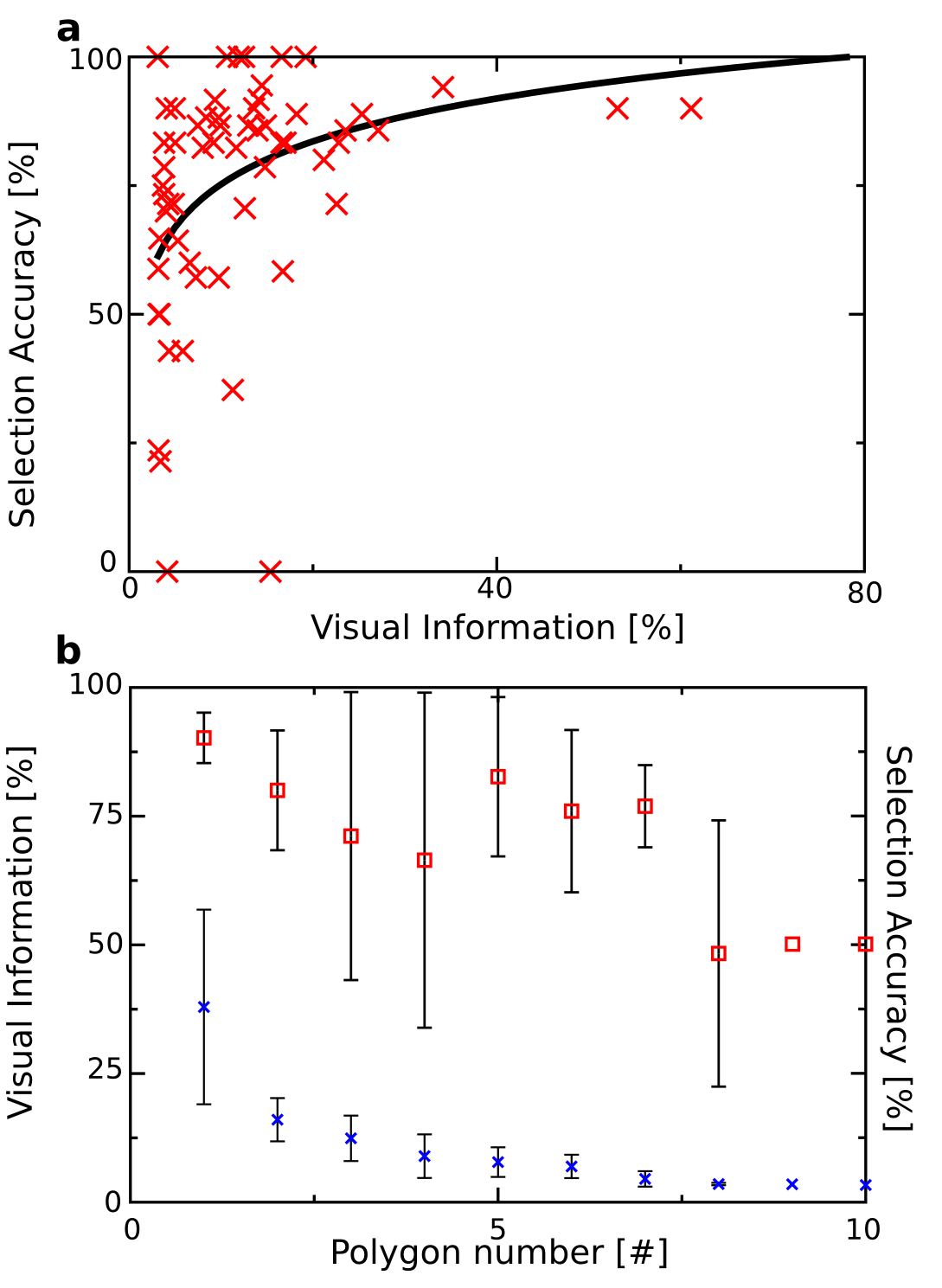
Figure 5: Performance drop with task difficulty. a Selection accuracy vs. visual information for individual polygons across subjects. Polygons bearing more information are usually larger, remind tightly in shape and color to their target, and are consequently easier to identify. Smaller polygons might reconstruct tiny details or refine existing shapes. These bear less visual information and represent a greater challenge for the image reconstruction, as indicated by the drop of performance for less information bearing polygons (thick, black trend line). It is remarkable, though, that a diversity of polygons with little visual information exists: some of them are correctly recognized almost always and some others are definitely tough to classify for any subject. b Visual information (blue crosses) and selection accuracy (red squares) vs. rank that each polygon occupies in the reconstruction of its target. Error bars indicate standard deviation of the values across polygons. Polygons presented later convey less information and are consequently more difficult to recognize in average. However, there is a huge variability in selection accuracy and a marked drop around polygons $4$ and $5$. Both panels were elaborated using data from experiments with $10$ blocks per burst. There is not any remarkable difference considering similar plots that include all data.

Because the right polygon was always preserved despite the outcome of the classifier, we could proceed with each reconstruction until the end and analyze the performance of the BCI as it explores more complicated scenarios in which target polygons convey very little information (down to $3\%$). As a result we found the selection accuracy drop for polygons bearing less visual information about the target (figure 5). Besides the obvious decay in accuracy for less informative primitives, we observe an increase in heterogeneity. As we move towards more difficult tasks, a range of selection accuracies emerge: some less informative polygons are rarely (two of them never) recognized as part of the target image while others are still correctly selected to a great extent. Polygons bearing more visual information tend to be accurately selected most of the time. Only $6$ polygons have always been correctly selected, all of them had a visual information below $20\%$ and one of them is at the edge of the $3\%$ threshold. These results were obtained for the eight subjects with $10$ blocks per burst during the reconstruction task. The outcome considering all subjects is broadly the same.

In accordance with the experimental design, less informative polygons appear later in the reconstruction task, as shown in figure 5b. The selection accuracy almost always decays as a reconstruction proceeds. Remarkably, the selection accuracy for the first polygon is $87.3\%$ ($90.8\%$ for subjects with $10$ blocks per burst). In figure 5b we also see an unexpected drop (followed by a rise) of the selection accuracy for intermediate polygons. The reason for this is discussed in appendix B and relies on the particularly difficult task that polygons $3$ or $4$ of some reconstructions posed to the subjects.

3.4 Ambiguous polygons

In choosing our pictures for reconstruction, we want them to be iconic with easily recognizable parts and with as little overlap as possible. However, it cannot be avoided that some drawings (or parts of them) resemble some other one. This leads to an undesired effect during the experimental sessions: some polygons did not belong to the reconstruction of the target drawing, but they bore some resemblance to it and were often classified as target. Because these polygons are strictly non-targets, they were excluded from the selection accuracy results reported in section 3.2. This does not imply a malfunction of the classifier because such polygons could have tricked the subjects as well. These pieces introduce an interesting ambiguity as they could contribute to several reconstructions. We refer to them as ambiguous polygons.

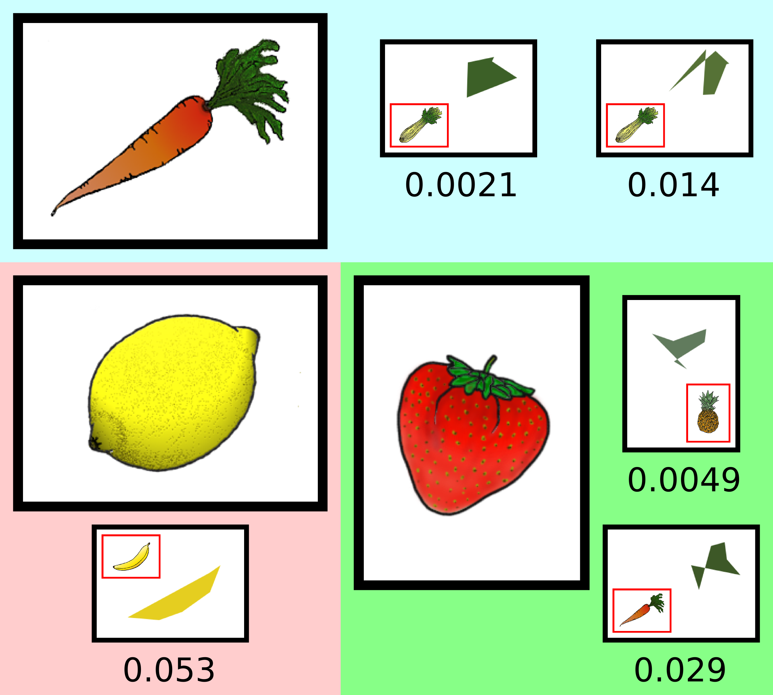
Figure 6: Ambiguous polygons. Some primitives could contribute to the reconstruction of different images. This could interfere with the reconstruction since these polygons would not be scored as correct classifications. The ambiguity of these pieces – that stems from the visual overlap between different targets – could be exploited to speed up the BCI image reconstruction. We shown the carrot, lemon, and strawberry together with some polygons that do not belong to their decompositions but that are overly selected by the classifier. For each polygon, within a red frame, it is shown the original drawing to which they belong. This figure was elaborated using data from experiments with $10$ blocks per burst. The scenario is similar if we use all data for this analysis.

As explained in section 2.3.1, along with each target polygon we chose $5$ non-target polygons from one common pool. One same polygon might have shown up several times as a non-target during one reconstruction, or for the reconstruction of the same drawing by different subjects. If in such cases the classifier repeatedly selected the non-target, we might have strong evidence that the subject perceives that polygon as contributing to the target drawing. Based on this, we computed $p$-values to ascertain what polygons had been more probably not selected by chance alone, but presumably because an honest interference existed between those non-targets and the target drawing. We show the top $5$ such pieces in figure 6 along with their $p$-values and the target images for which they were significantly over-selected. We see that these could perfectly contribute to sketch the target (like the polygon from the banana in the case of the lemon reconstruction) or to the refinement of a smaller detail (like the green polygons seemingly selected to complete the leaves of the carrot and the strawberry). In these paradigmatic cases the wrongly classified non-targets would show up roughly in the same area as the actual target polygons.

4 Discussion

In this paper we show how Rapid Serial Visual Presentation using bursts of polygons together with the oddball paradigm can be used for BCI image reconstruction. Our purpose was merely to attain a proof of concept. For that end, different design choices have been made and tested during the experimental sessions. A systematic search of the best working settings was never intended and is left for future work. Notwithstanding this, the results reported in section 3 invite us to be optimistic about the paradigm and demand that further, more rigorous experiments be performed. In this section we comment on our results and compare them to previous approaches to BCI-painting. We also propose future lines of research focusing on the development of a free-painting BCI based on the current paradigm.

4.1 Classification accuracy, performance drop, and comparison with previous research

In section 3.2 we reported a classification accuracy of $74.4\%$ ($76.4\%$ for subjects with $10$ blocks). This rises to $80.5\%$ ($83.4\%$) if we acknowledge that some correct classifications are more important than others, and use the percentage of visual information retrieved to weight our results. This means that we can reproduce up to $80\%$ of the visual information that the polygon decompositions capture of the original images.

These numbers would gain relevance if compared with those of other BCI-painting paradigms. We attempt this now, but a series of limitations exist due to the differences in BCI designs. For example, the guided evolution in [13] towards images that produce ‘positive’ feelings cannot be properly quantified. The authors report a $61\%$ accuracy, but this might be a biased result. After three generations of the genetic algorithm (which takes around $36$ minutes), subjects in [13] were asked to recall their actual choices – those picture that elicited more ‘positive’ feelings according to their conscious experience. Unfortunately, this approach is biased: the image selected by the classifier is used to generate variations that are then persistently shown to the subject, while the un-selected pictures are lost. One further limitation to compare our results to this work was pointed out at the introduction: in [13], there are no correlates with actual visual structures. While we quantify the overlap of our reconstructions with the original drawing (though naively, through the visual information), pictures in [13] evolve towards positive-looking images according to physiological feedback. Guiding the evolution towards visual details that we could quantify is rather difficult.

The impressive classification accuracy obtained in [14] clearly outperform ours. This work shall be a good reference for future BCI-painting paradigms, especially if it is possible to attain their high presentation rate ($8$ images per second during each burst) while keeping up in selection accuracy when the design is tested in actual image evolution tasks. Comparison with other aspects of our work is more difficult and we have to wait until this image evolution paradigm is put to an online test. Then, we will be able to study a sense of progression towards a final target and we could quantify properly how well detailed visual arrangements get reconstructed. If the accuracy results reported in [14] persist, this is a truly promising scheme.

Finally, the P300-Brain Painting BCI [16, 17, 18] performs very well in selection accuracies and it also provides two measures of $ITR$, reporting values that beat our BCI design. This is a very promising paradigm that mimics the equally successful matrix spellers. However, a few points should be considered. In usual spellers, a sentence is provided for a subject to copy. In [18], a picture is produced if we follow a series of instructions precisely: these indicate what shape to place next on the canvas, what color and size it shall be, and where it must be placed – all these instructions are stored as symbols in the matrix interface. These are the symbols that are accurately retrieved from the matrix for the results in [18] to make sense. Hence this is an instruction-copying task rather than a copy-painting one. If, otherwise, a subject were provided an image and were requested to copy-paint it, there would be several different sets of instructions leading to the same outcome, and such variations are more complicated to account for in terms of symbol accuracy. A similar problem restricts our BCI so that we have to dismiss ambiguous polygons, as explained above. While this implies some limitations for our paradigm, the problem is lightly deeper in [18]: copying a set of symbols (instructions) does not necessarily relate to visual cues on the canvas and, accordingly, makes quantification of the result more difficult. Specifically, it is not straightforward to find a meaningful measure equivalent to our visual information. While our selection accuracy and, specifically, our weighted accuracy report directly about the objective overlap that we attain with an actual target drawing, the results in [18] are more difficult to quantify in visual space.

We expect that future research on BCI-painting will make possible a more systematic comparison between different paradigms and visual outcomes. There is, though, a relevant caveat of our own BCI that deserves a closer analysis. In section 3.3 we report a performance drop as the difficulty of the task increases. Because of this, only $25\%$ of the reconstructions could proceed as intended. This should be improved in future implementations of the paradigm, and hence a series of alternatives are available:

• The rather conservative experimental settings (SOAs, some display options for the polygons, number of blocks per burs, etc) make possible an improvement to achieve faster $ITR$ and equally better accuracies. Gaining a few seconds per burst could allow us to introduce some error correcting mechanism, as discussed below, while keeping a high $ITR$.

• The classification results in [14] might be traced back to an easy cognitive task: $94\%$ of the bursts containing a target are consciously detected by the experimental subject, perhaps because the classification involves a clear-cut task. In our case (due to the presence of ambiguous situations) conscious wrong decisions might be prominent. This strongly suggests that to improve our accuracy we should pay more attention to the input stimuli. We could either exploit the role of ambiguous polygons or attempt to ban them altogether by building orthogonal primitives that produce a maximum diversity of designs with a minimum number of patterns. An interesting alternative could be to separate the generation of new shapes and their filling with color. This is an open and interesting problem at the frontier between BCI and natural image decomposition.

Admittedly a $25\%$ complete reconstructions falls short, but we suggest that this is not the best indicator of the performance of the BCI. It is desirable to complete the reconstruction of an image but this is a very stringent condition: finer grained primitives become more difficult to classify, while they might not be as important as the overarching primitives. Tinier details might also be open to more subjective appreciations by the BCI users. Furthermore, towards the end of a reconstruction the quality of the current primitives might degenerate since the genetic algorithm favors convergence of broad details first. We believe that weighting the classification accuracy by the amount of visual information that each classification contributes is a better indicator of the performance of our BCI paradigm. Then, as reported in section 3.2, up to $65.3\%$ ($68.3\%$ for subjects with $10$ blocks per burst) of visual information can be retrieved before the first classification mistake.

4.2 Moving towards a free-painting BCI

If we wanted to move towards an RSVP-based free-painting BCI machine, we could exploit the existence of ambiguous primitives and we should consider seriously the necessity of error correcting mechanisms. Other improvements should direct the evolution in an active way, avoiding full reliance on the randomness of primitives as discussed below, e.g., for the $2$-D location of new polygons. We speculate about the future of free-painting BCIs based on our paradigm in the following.

We consider first the possibility of including error correcting mechanisms to improve the classification accuracy and $ITR$. In computing the speed/accuracy trade-off by the $ITR$ formula, we neglected the problem of explicit correction of false BCI selections. These corrections that would have to be performed explicitly by the user are more time consuming than being accounted for by that equation (which assumes optimal error robust coding). Accordingly, a realistic trade-off would result in a higher number of blocks than the three suggested by figure 4b, reflecting the delay introduced by error correction. Other RSVP tasks have mechanisms to correct for wrong outputs. In RSVP spellers, a symbol can be explicitly incorporated among the letters to represent the backspace [19]. A similar approach could be taken for the present BCI application but it would likely interfere with the display of polygons. An appealing alternative are error potentials, a large scale signal elicited by unexpected feedback after a classification task, which can be used to automatically cancel incorrect selections [29].

One further alternative is inspired by [30] where ERP-based BCIs are explored. The selection accuracy is well characterized and a confirmation step (based on a similar RSVP task) is analyzed rendering a $96.26\%$ success with no false positives. Incorporating one such confirmation step would raise our selection accuracy to $82.1\%$. For this we computed the probability (across all subjects) that the second highest ranked polygon was the correct one given that the first choice was a wrong classification – this spares us a second burst but has a lower accuracy. If we would incorporate two confirmation steps (and, consequently, use the probability that the correct polygon was the third highest ranked one, provided the two first were not), the selection accuracy would rise to $87.8\%$. Alternatively, we could proceed with a second burst discarding the first (wrongly selected) polygon and introduce a new non-target one. This way, the accuracy would reach a $90.2\%$ for just one confirmation step. To include these details in an estimation of the $ITR$ would be very speculative: we should take into account not only the increased time lapse of the error correction task, but also potential undesired effects due to the disruption of the main painting task.

Before using solutions that need more steps, as the error correcting mechanisms discussed, we note that some available, relevant information is dismissed in the current design. A winner-takes-all decision is forced at the end of each burst while it is possible that several polygons get large scores from the classifier, especially if ambiguous primitives are present. On the other hand, easier classification at the beginning of a reconstruction might have a clear winner early in the burst. We could quantify the uncertainty of a decision (e.g. through an entropy-based classifier) and exploit this information, which is already captured by our BCI. The length of a burst could be dynamically tuned until the confidence of a decision would rise above a threshold. A sustained uncertainty could be taken as ‘select nothing’, an interesting option that free-painting applications should allow.

Regarding ambiguous polygons, these are pieces that might contribute to the reconstruction of several different images as reported in section 3.2. Usually, this is because the original drawings themselves share some common traits, as in the case of the green leaves located around the same position for the carrot, the strawberry, etc (figure 5). They do not represent a generalized situation: it would just affect a few polygons, and scoring these cases as correct classifications would not change our selection accuracy significantly.

For our results, these ambiguous polygons had a negative effect because they do not count as correct classifications (and thus lower our selection accuracy); but in a wider scope they might be extremely useful. While we imposed that the image decomposition be unique for each drawing, we can conceive of intermediate decompositions of multiple images with shared primitives. Then, a reconstruction should proceed from ambiguous, generalized descriptions towards more particular ones. This would establish a hierarchy that would cluster together pictures that are closer to each other in visual terms. By exploiting this feature we could discard non-targets quickly if they are very distant from our target but, as a consequence, we will progress towards more difficult classification tasks. To work out this situation we must research what is the finer detail that our BCI paradigm is able to resolve.

Linked to this, we could seek the use of maximally discriminating primitives at each reconstruction stage. Note the few constraints that we imposed upon the bursting polygons: many might be displayed within the same burst that convey redundant information, thus diminishing the exploratory capabilities of RSVP. Also, shape and color are tightly linked together in the current design. A two-stage decision that separates these arguably orthogonal features might be of great help towards a free-painting BCI. How we should design our primitives to maximally exploit the current paradigm is one of the open research lines proposed for the future.

Finally, there is an important aspect that is left to random chance in the current paradigm that should be corrected, if we really wanted our BCI users to explore freely the space of possible drawings. Right now, correct polygons are placed where they belong because their location is part of the specifications of each polygon decomposition. If we did not know the correct location of a primitive, it is extremely unlikely that it would be placed at the right spot by chance alone.

We envision the next design: Instead of the whole screen, consider a bursting area, a rectangle of restricted size laid upon the canvas within which all bursting polygons fit. Accordingly, the drawing will only suffer modifications in the framed area. The position and size of the bursting area could be controlled by a joystick, but this would not be appropriate for impaired users. Instead, the position of the frame could be modified through an eye tracking device or by sensory motor rhythms (as proposed in [18] for the P300-Brain Painting BCI). This last option would be the preferred choice for patients who cannot focus their sight (e.g. those suffering completely locked-in syndrome), but in this last case the drawing beneath the bursting area should be displaced while the bursting area remains fixed under the focus of the BCI user. Note that bursting is halted while the bursting area is manipulated.

To control the size of the bursting area when a joystick is not a viable option, we propose using the edges of the canvas as part of the interface: bringing the bursting area to the left-most edge of the canvas and insisting that it moves further than allowed would enlarge the horizontal dimension of the frame, while moving it all the way to the right and insisting that it goes further (e.g. focusing the sight outside the canvas region) would diminish the horizontal dimension. The same scheme would work for increasing/decreasing the vertical dimension using the top and bottom edges respectively, and the top-left and bottom-right corners would operate on both dimensions at the same time. We propose also that the top-right and bottom-left corners could be used to zoom in and out the canvas – note that this is strictly different from enlarging/shrinking the bursting area, since it allows for control over ever tinier details while the bursting polygons appear large to the BCI user.

Locating polygons in depth seems to be the remaining challenge. If necessary, we could dismiss the simultaneous modification of horizontal and vertical dimension and use the top-left and bottom-right corners to increase/decrease the layer where new primitives are bursting.

Appendix A Discussion of important design choices

A.1 Preprocessing of target images

Both writing and painting are emergent processes, although at very different levels. While in the former minimal components are clearly identified (written characters, letters) the latter is a truly emerging outcome of the very strongly, non-linearly interacting pieces that compose an image. It may be impossible to come down to some basic components of a drawing. If we intend to produce a picture from scratch, our choice of building blocks (say our alphabet for drawing) conditions the complexity that can be generated, the difficulty required to render each picture, and the speed to which we can produce it. We need to find adequate primitives that can compose a range of images quickly by combining the minimal units. Our pieces should be simple and schematic, and as pivotal to our targets as letters are to writing. We think that this is an open problem. For this study we adopted a provisional solution that we describe in the following.

As targets for reconstruction we sought iconic images from the Snodgrass and Vanderwart’s object database [23]. The chosen pictures (figure 1) are drawings of fruits and vegetables with basic shapes and colors; all of them laid on a white background, so that the reconstruction focuses in clear motives and not in peripheral details. Note anyway that the subject’s attention is free to wander over the screen. We discuss subject focus again in section A.2 in comparison with previous RSVP applications.

We need schematic, yet faithful, representations of the selected pictures. That was a preprocessing step completed weeks before the experiments. To extract useful primitives from our pool of drawings we found the perfect tool in recent applications of genetic algorithms (GAs) for image decomposition [24]. Such algorithms proceed through mutation and artificial selection from an arbitrary population of polygons to a set of polygons carefully arranged as to mimic a desired image.

For a GA, a fitness function needs to be introduced. Take a set of random polygons laid upon a white background, and some on each other to create a sense of depth. These compose an arbitrary image. Given an RGB color scheme, we use as fitness function the pixel-by-pixel Euclidean distance between the original picture and the image rendered by the collection of polygons. The better the fitness, the closer the collection of polygons resembles the original image.

As a seed for the algorithm we use an arbitrary collection of polygons $p_{i=0}=\{p_{0,j};j=1,\dots,n_{i}\}$, where $i$ labels iterations and $j$ labels the $n_{i}$ polygons composing the collection. Note that $n_{i}$ might change from one iteration to another. At each iteration the fitness of the current collection $P_{i}$ is evaluated. Some mutations are applied to generate an alternative polygon composition $P^{\prime}_{i}$. The collection with better fitness is retained: $max_{F}\{F(P_{i}),F(P^{\prime}_{i})\}\rightarrow P_{i+1}$, where $F(x)$ stands for the fitness function. The algorithm continues until a satisfactory convergence towards the original image has been reached or until the fitness does not improve for several iterations. The collection $P_{i_{end}}$ when the algorithm halts is referred to as the polygon decomposition of the original image.

The possible mutations applied at each iteration are: removal of a polygon or insertion of a new random one; swapping two polygons (recall that some polygons overlay some others); random addition, deletion, or modification of polygon’s vertices; change of a polygon color. Details on the probability of each operation (provided along the code [25]) are not relevant as long as a satisfactory approximation of the original images is achieved (which was done, as appreciated in figure 1).

The algorithm allows options regarding the kind of polygons that could be used. This turned out to be very important. We wished to discard very complex pieces; therefore only polygons with $3$ to $7$ vertices were allowed. We did not use partially transparent polygons – as implemented by the $\alpha$ parameter in the RGB color scheme. This was a valid option for the original GA [24], but it introduced important non-linearities in the interactions between polygons. As an instance, if transparency were allowed it might happen that some desired color shows up only after two polygons have been stacked in the right position. If only one of the polygons were present, we would not get quite the exact shade. But our paradigm only allows one polygon at a time, so we would risk rejecting the right polygon because it does not show the final result yet. By using only opaque polygons we partially solved this problem.

Once an image has been decomposed in its primitives, the fitness function also offers a measure of the importance of each piece in the reconstruction. For each polygon $p_{j}\in P_{i_{end}}$ we compute the fitness function of the whole arrange of polygons, and the fitness of the same arrange when $p_{i}$ is removed. We defined the visual information carried by the polygon as the normalized drop in fitness. There is no intention of connecting this visual information to actual theoretical information measures.

Using this visual information we ranked the polygons for each of our original images and retained only those contributing more than a $3\%$ (or $15\%$, see section 2.3.2). This choice renders fine enough reconstructions (see figure 1). Adding more polygons would only help with very tiny details and would make the experiments unnecessarily tedious.

The oddball paradigm requires that target stimuli are presented intermixed with neutral stimuli. When an original image from our pool was chosen as the object for reconstruction, all the polygons in its polygon decomposition became target stimuli. As for neutral stimuli, we used a pool containing all the polygons belonging to the decomposition of all other drawings.

This decision made the reconstruction task a fair one. All the polygons in our pool of neutral stimuli have been generated following the same procedure, only they belong to the polygon decomposition of different images. Differences between the two classes would ideally arise from their belonging or not to the target decomposition. If we would use, e.g., completely random polygons as neutral stimuli these could take any aspect, obviously including shapes that would hardly contribute to the generation of natural images. Such instances could be readily identified when opposed to polygons that account for details of some natural image. The reconstruction task would be artificially simplified by a preselection that greatly reduced the uncertainty about the target primitives. The task would effectively become a recognition of the less random- looking polygon.

A.2 Experimental setup

The natural guidelines for our BCI design are the experiments with RSVP spellers by Acqualagna and Blankertz [3, 4]. These give us a vague idea of settings under which a BCI for image reconstruction could function. We chose rather conservative specifications, given the novelty of the procedure. For example, during RSVP a burst SOA of $330\>ms$ between consecutive polygons was used. This lapse includes $100\>ms$ during which a void stimulus was intercalated. These settings can be compared to the SOAs of $116$ to $83\>ms$ from [3, 4], where letters succeeded each other without inserting any voids. These differences (together with the good results reported here and those from RSVP spellers) suggest that there is room for improvement should we seek more ambitious experimental settings.

The original motivation to introduce RSVP to BCI spellers was that letters could be presented always at the focal point. Stimuli falling right in the visual focus of the subject show enhanced ERPs which are detected more easily. This is not an asset in our case: we must allow the subjects to focus on different areas of their visual field when peripheral details of the target images are being reconstructed. We did not impose any conditions on the focus of the subjects. Looking at the long term goals of this research, the interest of RSVP will be on its exploratory potential because of the random, combinatorial nature of the bursting primitives and its interplay with the subject’s (sub)conscious driving of the image reconstruction process. We are convinced that these ideas are worth exploring.

As indicated in section 2.4, occasionally, the intervals determined by the heuristic were adjusted by the experimenter before starting the on-line runs. These adjustments where generic for all subjects and intended to guide the classifier towards informative time intervals. In all cases, the linear classifier converged towards five discriminative temporal intervals (ideally towards the most discriminative ones), partly erasing the manual setup. Table 1 collects the eventual time intervals chosen by the classifier for each subject.

Table 1: Discriminative time intervals found by the linear classifier for each subject.

BCI subject:	$T_{1}$ [$ms$]	$T_{2}$ [$ms$]	$T_{3}$ [$ms$]	$T_{4}$ [$ms$]	$T_{5}$ [$ms$]
VPjam	$70-120$	$120-150$	$240-350$	$345-480$	$475-530$
VPmai	$110-160$	$360-390$	$385-500$	$495-590$	$585-810$
VPmao	$210-290$	$340-440$	$435-560$	$555-570$	$640-720$
VPmap	$100-130$	$160-200$	$195-280$	$275-470$	$465-530$
VPmaq	$220-400$	$395-440$	$435-650$	$645-680$	$680-760$
VPmar	$130-170$	$210-390$	$385-480$	$475-590$	$585-690$
VPmas	$240-350$	$450-500$	$550-620$	$615-680$	$675-770$
VPmat	$220-250$	$245-280$	$275-370$	$365-510$	$505-790$
VPmau	$210-250$	$290-320$	$315-450$	$445-560$	$600-660$
VPmav	$130-180$	$280-330$	$325-470$	$465-590$	$585-610$

For the present proof of concept, we focused on achieving a classification accuracy good enough, for which we took into account as much spatio-temporal information as possible. Underlying this choice are the patterns inferred by the classifier, which involve the activity of most channels available during a series of time intervals (see Table 1). However, the current design relies strongly on the P300 oddball paradigm whose macroscopic imprint is a frontal/central positive deflection of the scalp potential. More classic accounts of this signal rely on measurements on central electrodes alone, prominently on the Cz channel.

It is fair to ask whether these central channels alone have discriminative power to accomplish the image-reconstruction task of our BCI. In figure 7 we plot the average selection accuracy per channel if that channel alone were considered by the classifier. We observe that the central and fronto-central channels are the most predictive ones, strongly supporting that the P300 fronto-central potential underlies the analyzed ERP.

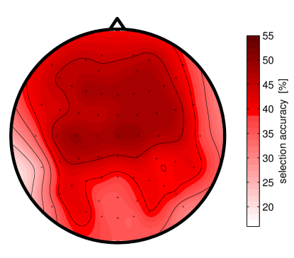
Figure 7: Selection accuracy scalp plot for a classifier trained on individual channels alone. This image reveals that the most informative channels occupy fronto-central positions (remarkably around the Cz channel), which is in accordance with a prominent role of the P300 ERP in the task under analysis. However, a notable drop in comparison with the accuracy of extended spatio-temporal filters indicates either that signals other than P300 are valuable, or that that signal is enhanced through implicit spatio-temporal filtering when data from many channels is available. We cannot decide between both possibilities currently.

We also observe a notable drop in classification accuracy compared to the quality obtained with compound spatio-temporal filters (below $50\%$ for all individual channels compared to $70\%$ and higher accuracies reported in the body of the paper). This might suggest a relevant role for other sources than the fronto-central channels. Notwithstanding, this does not imply that the enhanced accuracy of extended spatio-temporal filters necessarily stems from signals other than the P300 deflection. Due to the availability of data from multiple channels, the signal of interest may be enhanced by implicit spatial filtering. With the available data, we cannot distinguish between these possibilities.

Appendix B Average performance drop for intermediate polygons

In section 3.3 it was reported the performance drop as the difficulty of the reconstruction task increased. Two approaches were taken: i) The selection accuracy was plotted against the visual information carried by each polygon and ii) the selection accuracy was plotted as a function of the rank that each polygon occupied in the reconstruction. The first method asserts that the selection accuracy drops in average for polygons that contribute less to the reconstruction of the image (figure 5a). Highly informative polygons are usually correctly classified, but the least informative polygons display a great variation. Some of them are often well classified and some of them are not, with a range of selection accuracies in-between. This indicates that the reconstruction task does not always become more difficult as we move towards less informative polygons.

Figure 5b reports the average selection accuracy across all reconstructions against the rank that a given polygon occupies in the reconstruction. The reconstruction task proceeds from the most informative polygons to the least informative ones, given the target picture. The latter contain less information about the original image, and hence it should be more difficult to classify them correctly. Unexpectedly, the decay in performance is not a monotone function: polygons $5$, $6$, and $7$ in the reconstruction are selected with notably more accuracy than polygons $3$ and $4$. This indicates that there are some less informative polygons that are correctly selected more often than the average of other, more informative polygons.

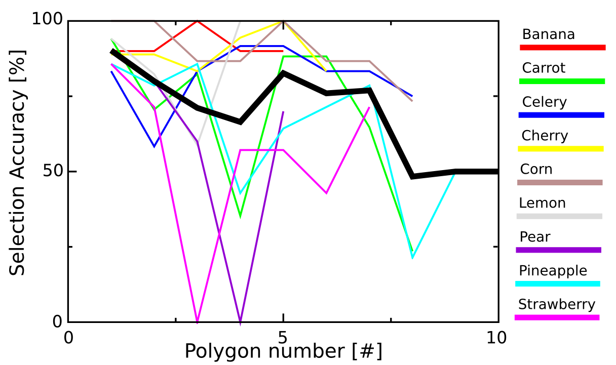
Figure 8: Performance drop in early polygons. Polygons appearing earlier in the reconstruction task bear more visual information about the targets than those showing up later. The former should be easier to recognize and be correctly classified more often. Despite this, there is a marked drop in selection accuracy of intermediate polygons when accuracy is averaged over all polygons with the same rank in the distribution (thick black line). We appreciate that the strawberry (magenta), the carrot (green), the pear (violet), and the pineapple (cyan) pose challenging tasks to the subjects precisely at polygons $3$ or $4$ of their decomposition, accounting for the average drop.

Figure 8 clarifies this drop in performance for intermediate polygons. When we look at the average accuracy per polygon for single reconstructions we note that some of them present a strongly marked fall in selection accuracy for polygons $3$ and $4$: the strawberry in polygon $3$; and the carrot, the pear, and the pineapple in polygon $4$. All four cases present a selection accuracy lower than $50\%$ for these polygons, contributing to an average performance drop across reconstructions. These polygons happen to be just difficult to classify.

In two of these cases (strawberry and pear) the problematic polygons are very light gray pieces that contribute to the reconstruction (perhaps by occluding some spurious detail brought in by earlier pieces, as with the third polygon of the cherry [26]). Because they are almost white, they are easy to miss against the blank background. In the case of the carrot the performance drop is not so dramatic. Also, this polygon number $4$ contributes to the leaves of the carrot and, as we saw in section 3.4, that was precisely a common location of ambiguous polygons. If some ambiguous non- targets have been overly miss-classified, some actual targets must necessarily be missed.

Nothing remarkable has been recognized in the case of the pineapple: the conflicting polygon seems to be a working, non-ambiguous piece of the reconstruction and we just assume that this precise primitive was more difficult for the subjects (note that the performance raises back to average for polygons $6$ and $7$ of the pineapple). Among the four important deviations at intermediate stages, this is the case with the lowest drop.

References

- [1] Patel SH, Azzam PN, Characterization of N200 and P300: selected studies of the event-related potential. Int. J. Med. Sci. 2, 147-154 (2005).
- [2] Polich J, Updating P300: an integrative theory of P3a and P3b. Clin. Neurophysiol. 118, 2128-2148 (2007)
- [3] Acqualagna L and Blankertz B, A novel brain-computer interface based on the rapid serial visual presentation paradigm. Conf. Proc. IEEE Eng. Med. Biol. Soc., 2686-2689 (2010).
- [4] Acqualagna L and Blankertz B (2013). Gaze-independent BCI-spelling using rapid serial visual presentation (RSVP). Clin. Neurophysiol. 124, 901-908.
- [5] Ahani A, Wiegand K, Orhan U, Akcakaya M, Moghadamfalahi M, Nezamfar H, Patel R, Erdogmus D, RSVP IconMessenger: icon-based brain-interfaced alternative and augmentative communication. Brain-Computer Interfaces 1(3-4), 192-203 (2014).
- [6] Gerson AD, Parra LC, Sajda P, Cortically-coupled computer vision for rapid image search. IEEE Trans. Neural Syst. Rehabil. Eng. 14, 174-179 (2006).
- [7] Parra LC, Christoforou C, Gerson AD, Dyrholm M, Luo A, Wagner M, Philistiades MG, Sajda P, Spatiotemporal lineaer decoding of brain state: application to performance augmentation in high-throughput tasks. IEEE Signal Process. Mag. 25, 95-115 (2008).
- [8] Sajda P, Pohlmeyer E, Wang J, Parra LC, Christoforou C, Dmochowski J, Hanna B, Bahlmann C, Singh MK, Chang S-F, In a blink of an eye and a switch of a transistor: cortically coupled computer vision. Proc. IEEE 98, 462-478 (2010).
- [9] Bigdely-Shamlo N, Vankov A, Ramirez RR, Makeig S, Brain activity-based image classification from rapid serial visual presentation. In Neural Systems and Rehabilitation Engineering, IEEE Transactions on, 16(5), 432-441 (2008).
- [10] Huang Y, Erdogmus D, Pavel M, Mathan S, Hild II KE, A Framework for Rapid Serial Visual Image Search using Single-trial Evoked Responses. Neurocomputing 74(12), 2041-2051 (2010).
- [11] Pohlmeyer EA, Wang K, Jangraw DC, Lou B, Chang S-F, Sajda P, Closing the loop in a cortically-coupled computer vision: a brain–computer interface for searching image databases. J. Neural Eng. 8, 036025 (2011).
- [12] Ušćumlicć M, Chavarriaga R, Millán JdR, An Iterative Framework for EEG-based Image Search: Robust Retrieval with Weak Classifiers. PLoS one 8(8), e72018 (2013).
- [13] Basa T, Go CA, Yoo K-S, Lee W-H, Using Physiological Signals to Evolve Art. In Applications of Evolutionary Computing (pp. 633-641). Springer Berlin Heidelberg, (2006).
- [14] Shamlo NB, Makeig S, Mind-Mirror: EEG-Guided Image Evolution. Novel Interaction Methods and Techniques (pp. 569-578). Springer Berlin Heidelberg, (2009).
- [15] http://www.picbreeder.com
- [16] Kübler A, Halder S, Furdea A, Hösle A, “Brain Painting – BCI meets art”, in Proceedings of the 4th International Brain-Computer Interface Workshop and Training Course, 361-366 (2008).
- [17] Halder S, Furdea A, Leeb R, Müller-Putz G, Hösle A, Kübler A, “Implementation of SMR based brain painting”. Poster at Neuromath Workshop. Leuven, Belgium (2009).
- [18] Müs̈inger JI, Halder S, Kleih SC, Furdea A, Raco V, Hösle A, Kübler A, Brain Painting: First Evaluation of a New Brain–Computer Interface Application with ALS-Patients and Healthy Volunteers. Front. Neurosci. 4, 182 (2010).
- [19] Farwell LA, Donchin E, Talking off the top of your head: toward a mental prosthesis utilizing event-related brain potentials. Electroencephalogr. Clin. Neurophysiol. 70, 510 (1988).
- [20] Venthur B, Scholler S, Williamson J, Dähne S, Treder MS, Kramarek MT, Müller K-R, Blankertz B, Pyff—A Pythonic Framework for Feedback Applications and Stimulus Presentation in Neuroscience. Frontiers Neurosci. 00179, doi: 10.3389/fnins.2010 (2010).
- [21] http://www.pygame.org
- [22] Straw AD, Vision Egg: An Open-Source Library for Realtime Visual Stimulus Generation. Frontiers Neuroinformatics, doi: 10.3389/neuro.11.004.2008 (2008).
- [23] Rossion L, Pourtois G, Revisiting Snodgrass and Vanderwart’s object database: Color and Texture improve Object Recognition. J. of Vision 1(3), 413 (2001).
- [24] http://alteredqualia.com/visualization/evolve/ https://code.google.com/p/alsing/downloads/list
- [25] https://github.com/dedan/poly_burst
- [26] http://youtu.be/LERyK3z2cYs
- [27] Lemm S, Blankertz B, Dickhaus T, Müller KR, Introduction to machine learning for brain imaging. Neuroimage 56(2), 387-399 (2011).
- [28] McFarland DJ, Wolpaw JR, EEG-based communication and control: Speed-accuracy relationships. Appl. Psychophysiol. Biofeedback 28(3), 217-231 (2003).
- [29] Schmidt N, Blankertz B, Treder MS, Online detection of error potentials increases information throughput in a brain-computer interface. Neurosci Lett, 500(1), 19-20 (2011).
- [30] Lorenz R, Pascual J, Blankertz B, Vidaurre C, Towards a holistic assessment of the user experience with hybrid BCIs. J Neural Eng, 11(3), 035007 (2014).