A Forward Equation for Barrier Options under the Brunick&Shreve Markovian Projection

Abstract.

We derive a forward equation for arbitrage-free barrier option prices in continuous semi-martingale models, in terms of Markovian projections of the stochastic volatility process. This leads to a Dupire-type formula for the coefficient derived by Brunick and Shreve for their mimicking diffusion and can be interpreted as the canonical extension of local volatility for barrier options. Alternatively, a forward partial-integro differential equation (PIDE) allows computation of up-and-out call prices under such a model, for the complete set of strikes, barriers and maturities from a single equation. In the same way as the vanilla forward Dupire PDE, the above-named forward PIDE can serve as a building block for an efficient calibration routine including barrier option quotes. We propose a discretisation scheme for the PIDE as well as a numerical validation.

1. Introduction

Efficient pricing and hedging of exotic derivatives requires a model which is rich enough to re-price accurately a range of liquidly traded market products. The case of calibration to vanilla options is now widely documented and has been considered extensively in the literature since the work of Dupire [10] in the context of local volatility models (see also Gyöngy’s formula [18]). Nowadays, the exact re-pricing of call options is a must-have standard, and LSV (local-stochastic volatility) models are the state-of-the-art in many financial institutions because of their superior dynamic properties over pure local volatility. Various sophisticated calibration techniques are in use in the financial industry, for example, based on the work of Guyon and Labordère [17] as well as Ren, Madan and Qian [20]. However, practitioners are increasingly interested in taking into account the quotes of touch and barrier options as well; the extra information they embed can be valuable in obtaining arbitrage-free values of exotic products with barrier features.

A few published works already address this question from different angles and under different assumptions. For example, in Crosby and Carr [5] a particular class of models gives a calibration to both vanillas and barriers. Model-independent bounds on the price of double no-touch options were inferred from vanilla and digital option quotes in Cox and Obloj [7]. Pironneau [19] proves that the Dupire equation is still valid for a given barrier level, in a local volatility setting. The direct generalisation of this result to general stochastic volatility models appears not to be straightforward.

In our work, we approach the problem from the Brunick-Shreve mimicking point of view [3] in the general framework of continuous stochastic volatility models. We derive a condition to be satisfied by the expectation of the stochastic variance conditional on the spot and its running maximum, $\mathopen{}\mathclose{{}\left(S_{t},M_{t}}\right)$, in order to reproduce barrier prices. This conditional expectation is often referred to as a Markovian projection. For simplicity, we focus on up-and-out call options with no rebate and continuous monitoring of the barrier, but the analysis extends to other payoff types. In the case of double barrier options, one would also have to consider the running minimum leading to an additional dimension and boundary term.

The derivation is inspired by the work of Derman & Kani [9] and Dupire [10, 11]. In that context, Gyöngy’s mimicking result [18] provides the financial engineer with a recipe to build a low-dimensional Markovian process which reproduces exactly any marginal density of the spot price process for all times $t$. Brunick and Shreve [3] extend Gyöngy’s result to path functionals of the underlying process, of which the running maximum is a special case. In particular, they prove for any stochastic volatility process the existence of a mimicking low-dimensional Markovian process with the same joint density for $\mathopen{}\mathclose{{}\left(S_{t},M_{t}}\right)$.

In [13], Forde presents a way to retrieve the mimicking coefficient by deriving a forward equation for the characteristic function of $\mathopen{}\mathclose{{}\left(S_{t},M_{t}}\right)$; computation of the coefficient is possible via an inverse two-dimensional Fourier-Laplace transform. Here, we present an alternative method to retrieve the mimicking coefficient, which lies closer to the well-known Dupire formula and can hence benefit from the earlier work in the field of vanilla calibration.

We derive a partial-integro differential equation (PIDE) in strike, barrier level and maturity for up-and-out calls priced under the Brunick-Shreve model. This forward differential equation has the same useful properties (and drawbacks) as the Dupire forward PDE. As a consequence, it can be used to price a set of up-and-out calls in one single resolution. In this regard, our method shares some similarities with the forward equations derived by Carr and Hirsa [6]. We highlight a few key differences though. First, we consider the class of stochastic volatility models rather than local volatility models with a jump term. In working directly with Brunick and Shreve’s Markovian projection onto $\mathopen{}\mathclose{{}\left(S_{t},M_{t}}\right)$, we need to consider the running maximum explicitly in our derivation. This complicates the proof and makes the idea used in [6] – employing stopping times – not applicable in our case. For the above type of Markovian projection, one gets an unusual “integro” term in the PIDE involving a second derivative, which requires particular care in the numerical solution. In contrast, the “integro” term in [6] comes from the jump process and is not treated in the same way as ours.

A very recent paper by Guyon [16] explains how path-dependant volatility models, like the Brunick-Shreve one, may be very useful to replicate a market’s spot-volatility dynamics, in particular highlighting the running maximum. It is important to note, though, that the diffusion of interest can be a fairly general stochastic process in our framework. More specifically, the variance process does not need to contain the running maximum in its parametrisation, and we do not particularly advocate the dynamic use of such a model here. Indeed, by doing so, one may find oneself with the logical conundrum that the model for the underlying depends on the time of inception of the option, i.e., the time the clock starts for the running maximum. The view we take here is that the Brunick-Shreve projection is a “code book” (to borrow a term from [4]) for barrier option prices, to which other models may be calibrated. Additionally, the forward PIDE enables in principle the pricing over a wide set of up-and-out call deals, creating a possible efficient direct solver for the inverse problem, i.e., to retrieve model parameters from any desired model class via the projected volatility $\sigma\mathopen{}\mathclose{{}\left(S_{t},M_{t},t}\right)$.

The remainder of this paper is organised as follows. In Section 2, we introduce the modelling setup and hypotheses and derive, as our first main result, a forward equation (in terms of the maturity) for barrier option prices, where the strike and barrier levels are spatial variables. Next, in Section 3, we derive a Dupire-type formula for barrier options, leading to a known setup for the reader familiar with vanilla calibration. In order to build the first step of a calibration routine to reprice up-and-out call options, we deduce a forward PIDE in Section 4 with better stability properties and develop a numerical solution scheme. Finally, in Section 5, we show that the forward PIDE and the “classical” backward pricing PDE agree on the price of barrier options, which validates our approach. Section 6 concludes.

2. Setup and Main Result

We consider a market with a risk-free, deterministic and possibly time-dependent short rate, $r(t)$ at time $t$, and continuously compounded deterministic dividend $q(t)$. Then $D\mathopen{}\mathclose{{}\left(t}\right)=\exp(-{\int_{0}^{t}r\mathopen{}\mathclose{{}\left(u}\right)\,du})$ is the discount factor, and $Q\mathopen{}\mathclose{{}\left(t}\right)=\exp({\int_{0}^{t}q\mathopen{}\mathclose{{}\left(u}\right)\,du})$ is the dividend capitalisation.

We assume the existence of a filtered probability space ($\chi$, $\mathcal{F},\mathopen{}\mathclose{{}\left\{\mathcal{F}_{t}}\right\}_{t\geq 0},\mathbb{Q})$ with a (not necessarily unique) risk-neutral measure $\mathbb{Q}$, under which the price process of a risky asset follows

(2.1) $$\frac{dS_{t}}{S_{t}}=\mathopen{}\mathclose{{}\left(r\mathopen{}\mathclose{{}\left(t}\right)-q\mathopen{}\mathclose{{}\left(t}\right)}\right)\,dt+\alpha_{t}\,dW_{t},$$

where $W$ is a standard Brownian motion and $\alpha_{t}$ is a continuous and positive $\mathcal{F}_{t}$-adapted semi-martingale such that

(2.2) $$\mathbb{E}^{\mathbb{Q}}\mathopen{}\mathclose{{}\left[\int_{0}^{t}\alpha_{u}^{2}S_{u}^{2}\ du}\right]<\infty.$$

A practically important example is $\alpha_{t}=f\mathopen{}\mathclose{{}\left(S_{t},t}\right)\sqrt{V_{t}}$ with a local volatility function $f$ and a CIR process $V$, which is often referred to as a local stochastic volatility (LSV) model.

In this paper, we consider an up-and-out call option on $S$ with continuously monitored barrier $B$, strike $K$, and maturity $T$. The arbitrage-free price under $\mathbb{Q}$ is

$$C\mathopen{}\mathclose{{}\left(K,B,T}\right)=\mathbb{E^{\mathbb{Q}}}\mathopen{}\mathclose{{}\left[D\mathopen{}\mathclose{{}\left(T}\right)\mathopen{}\mathclose{{}\left(S_{T}-K}\right)^{+}\mathbf{1}_{M_{T}<B}}\right],$$

where $\mathbf{1}_{A}$ is the indicator function of event $A$ and

$$M_{t}=\underset{0\leq u\leq t}{\max}S_{u}$$

the running maximum process of $S$. Adaptations of our results to other types of barrier options (such as put payoffs, down-and-out barriers etc) are easily possible using a similar derivation to below.

We now derive the first main result which links the barrier option price to the Markovian projection of the stochastic volatility (2.1) onto the spot and its running maximum $\mathopen{}\mathclose{{}\left(S_{t},M_{t}}\right){}_{t\geq 0}$, which we define by

(2.3) $$\sigma_{|S,M}^{2}\mathopen{}\mathclose{{}\left(K,B,T}\right)=\mathbb{E^{\mathbb{Q}}}\mathopen{}\mathclose{{}\left[\alpha_{T}^{2}\mid S_{T}=K,M_{T}=B}\right].$$

A recent result by Brunick and Shreve [3], which we apply to the process $\log\mathopen{}\mathclose{{}\left(S_{t}}\right)$, shows that under the integrability condition (2.2) on $\alpha$, the function $\sigma_{|S,M}$ is measurable, and gives the existence of a one-dimensional “mimicking” process $\widehat{S}$ with running maximum $\widehat{M}$, such that for all $t$

(2.4) $$(S_{t},M_{t})\stackrel{{\scriptstyle law}}{{=}}(\widehat{S}_{t},\widehat{M}_{t}),$$

where $\widehat{S}$ is the weak solution of

(2.5) $$\frac{d\widehat{S}_{t}}{\widehat{S}_{t}}=\mathopen{}\mathclose{{}\left(r\mathopen{}\mathclose{{}\left(t}\right)-q\mathopen{}\mathclose{{}\left(t}\right)}\right)\,dt+\sigma\mathopen{}\mathclose{{}\left(\widehat{S}_{t},\widehat{M}_{t},t}\right)\,d\widehat{W}_{t},$$

with a standard Brownian motion $\widehat{W}$ on a suitable probability space, and

$$\sigma(K,B,T)=\sigma_{|S,M}(K,B,T).$$

Remark.

We can take two views of (2.5) from the perspective of derivative pricing. First, we can think of $\sigma$ in (2.5) as a model in its own right, with a local volatility which additionally depends on the running maximum – see [16] for a discussion of “path-dependent” volatility models. This extra flexibility of matching the path-dependence of the local volatility allows calibration to barrier contracts as well as vanillas, yet keeps the market complete.

Second, and more common, a different volatility model may be used, for instance the aforementioned LSV model. In that case, the mimicking Brunick-Shreve model will give the same barrier option prices as the higher-dimensional diffusion as barrier option values are characterised precisely by the joint distribution of spot and running maximum. This property is important for calibration purposes as we will describe later. In either case, $\sigma$ plays a similar role for barrier options as the Dupire local volatility does for vanillas.

Assumption 1.

We assume that $\sigma$ in (2.5) is bounded and $C^{2,1,0}(\Omega\times\mathbb{R}^{+})$. This implies that $(\widehat{S},\widehat{M})$ is Markovian (see [2]; bounded and locally Lipschitz is sufficient). We also assume that $(S_{t},M_{t})$ – or, equivalently, $(\widehat{S}_{t},\widehat{M}_{t})$ – has a twice differentiable transition density $\phi$ under $\mathbb{Q}$, with bounded derivatives.

Proposition 1.

Under Assumption 1, the density $\phi$ is the classical solution of the following Kolmogorov forward equation in the region $\Omega=\{(x,y):0<x<y,S_{0}<y\}$,

(2.6) $$\frac{\partial\phi}{\partial t}+(r(t)-q(t))\frac{\partial}{\partial x}(x\phi)-\frac{1}{2}\frac{\partial^{2}}{\partial x^{2}}\mathopen{}\mathclose{{}\left(\sigma^{2}x^{2}\phi}\right) = 0,\qquad\qquad\qquad\;(x,y)\in\Omega,\;t>0,$$

(2.7) $$\frac{\partial}{\partial x}\mathopen{}\mathclose{{}\left(\sigma^{2}x^{2}\phi}\right)+\frac{1}{2}\frac{\partial}{\partial y}\mathopen{}\mathclose{{}\left(\sigma^{2}x^{2}\phi}\right) = (r(t)-q(t))\ x\ \phi,\qquad x=y,\;t>0,\!\!$$

(2.8) $$\phi(S_{0},S_{0},t) = 0,\qquad\qquad\qquad\qquad\qquad\;\;\;\;\;\;t>0,$$

$$\phi(x,y,0) = \delta(x-S_{0})\delta(y-S_{0}),\quad\quad(x,y)\in\Omega.$$

For completeness, we give a derivation of these equations in Appendix A.

This initial-boundary value problem is the adjoint to the backward equation satisfied by the option value $C$ as a function of $S_{t}$, $M_{t}$ and $t$, which has a homogeneous Neumann boundary condition on the diagonal $S=M$.

Remark.

The assumption of smoothness of the joint density is non-trivial. For the Black-Scholes model, with constant $\sigma$, the joint density function is known explicitly and smooth. In a recent work, [14] show the existence of the joint density – not necessarily differentiable – of an Itô process $X$ and its running minimum $\underline{X}$, where the local volatility is a sufficiently smooth and suitably bounded function of $X_{t}$ and $\underline{X}_{t}$. We also note that although the density features in our proof, it does not appear in the final result itself, and we conjecture that the regularity assumption may be weakened. Nonetheless, forward equations involving the transition density are widely used for calibration in practice and we envisage that (2.6) can also be a useful building block for calibration in the present framework. Therefore, it seems reasonable to require that the model has enough regularity for the density to satisfy such an equation.

The time zero value of barrier options can then be written as

(2.9) $$C(K,B,T) = D(T)\;\int_{S_{0}}^{\infty}\int_{0}^{\infty}(x-K)^{+}\mathbf{1}_{y<B}\,\phi(x,y,T){\,\rm d}x{\,\rm d}y$$

$$= D(T)\;\int_{K\vee S_{0}}^{B}\int_{K}^{y}(x-K)\,\phi(x,y,T){\,\rm d}x{\,\rm d}y.$$

We can now extend the argument from Dupire [10] for European calls to derive a forward equation for barriers.

Theorem 2.

Under (2.2) and Assumption 1, the value $C(K,B,T)$ of an up-and-out barrier call satisfies, for all $0<K<B$ and $T>0$,

(2.10) $$\frac{\partial^{2}C\mathopen{}\mathclose{{}\left(K,B,T}\right)}{\partial B\partial T}+\mathopen{}\mathclose{{}\left(r\mathopen{}\mathclose{{}\left(T}\right)-q\mathopen{}\mathclose{{}\left(T}\right)}\right)K\frac{\partial^{2}C\mathopen{}\mathclose{{}\left(K,B,T}\right)}{\partial K\partial B} = \frac{1}{2}\sigma_{|S,M}^{2}\mathopen{}\mathclose{{}\left(K,B,T}\right)K^{2}\frac{\partial^{3}C\mathopen{}\mathclose{{}\left(K,B,T}\right)}{\partial K^{2}\partial B}-q\mathopen{}\mathclose{{}\left(T}\right)\frac{\partial C\mathopen{}\mathclose{{}\left(K,B,T}\right)}{\partial B}\vspace{0.1 cm}$$

$$-\frac{1}{2}\frac{{\rm d}}{{\rm d}B}\mathopen{}\mathclose{{}\left(\mathopen{}\mathclose{{}\left(B-K}\right)B^{2}\sigma_{|S,M}^{2}\mathopen{}\mathclose{{}\left(B,B,T}\right)\mathopen{}\mathclose{{}\left.\frac{\partial^{3}C\mathopen{}\mathclose{{}\left(K,B,T}\right)}{\partial K^{2}\partial B}}\right\rfloor_{K=B}}\right)\,,$$

where $\sigma_{|S,M}$ is given by (2.3).

Proof.

Because of Brunick and Shreve’s mimicking result, (2.4) and (2.5), and the smoothness assumption, we can work with a density satisfying the forward equation (2.6) and (2.7). We denote $\mu\mathopen{}\mathclose{{}\left(t}\right)=r\mathopen{}\mathclose{{}\left(t}\right)-q\mathopen{}\mathclose{{}\left(t}\right)$. Differentiating (2.9) with respect to $B$ and $T$ in the first equation, using (2.6) in the second, and integrating by parts in the third, we obtain

$$\frac{\partial^{2}C\mathopen{}\mathclose{{}\left(K,B,T}\right)}{\partial T\partial B} = -r\mathopen{}\mathclose{{}\left(T}\right)\frac{\partial C\mathopen{}\mathclose{{}\left(K,B,T}\right)}{\partial B}+D\mathopen{}\mathclose{{}\left(T}\right)\int_{K}^{B}(x-K)\frac{\partial\phi}{\partial t}(x,B,T){\,\rm d}x$$

$$= -r\mathopen{}\mathclose{{}\left(T}\right)\frac{\partial C\mathopen{}\mathclose{{}\left(K,B,T}\right)}{\partial B}+$$

$$D\mathopen{}\mathclose{{}\left(T}\right)\int_{K}^{B}(x-K)\mathopen{}\mathclose{{}\left[-\mu\mathopen{}\mathclose{{}\left(T}\right)\frac{\partial}{\partial x}\mathopen{}\mathclose{{}\left(x\phi(x,B,T)}\right)+\frac{1}{2}\frac{\partial^{2}}{\partial x^{2}}\mathopen{}\mathclose{{}\left(\sigma^{2}(x,B,T)x^{2}\phi(x,B,T)}\right)}\right]{\,\rm d}x$$

$$= -r\mathopen{}\mathclose{{}\left(T}\right)\frac{\partial C\mathopen{}\mathclose{{}\left(K,B,T}\right)}{\partial B}+$$

$$\mu\mathopen{}\mathclose{{}\left(T}\right)D\mathopen{}\mathclose{{}\left(T}\right)\mathopen{}\mathclose{{}\left[-B\mathopen{}\mathclose{{}\left(B-K}\right)\phi\mathopen{}\mathclose{{}\left(B,B,T}\right)+\int_{K}^{B}\mathopen{}\mathclose{{}\left(x-K}\right)\phi(x,B,T){\,\rm d}x+K\int_{K}^{B}\phi(x,B,T){\,\rm d}x}\right]+$$

$$\frac{1}{2}D\mathopen{}\mathclose{{}\left(T}\right)\mathopen{}\mathclose{{}\left(\sigma^{2}(K,B,T)K^{2}\phi(K,B,T)-\sigma^{2}(B,B,T)B^{2}\phi(B,B,T)}\right)\ +$$

$$\frac{1}{2}D\mathopen{}\mathclose{{}\left(T}\right)(B-K)\mathopen{}\mathclose{{}\left[\frac{\partial}{\partial x}\mathopen{}\mathclose{{}\left(\sigma^{2}(x,B,T)x^{2}\phi(x,B,T)}\right)}\right]_{x=B}.$$

Using the boundary condition (2.7) in the second line of

$$\frac{{\rm d}}{{\rm d}B}\mathopen{}\mathclose{{}\left(\sigma^{2}(B,B,T)B^{2}\phi(B,B,T)}\right) = \mathopen{}\mathclose{{}\left[\frac{\partial}{\partial x}\mathopen{}\mathclose{{}\left(\sigma^{2}(x,B,T)x^{2}\phi(x,B,T)}\right)}\right]_{x=B}+\mathopen{}\mathclose{{}\left[\frac{\partial}{\partial B}\mathopen{}\mathclose{{}\left(\sigma^{2}(x,B,T)x^{2}\phi(x,B,T)}\right)}\right]_{x=B}$$

$$= -\mathopen{}\mathclose{{}\left[\frac{\partial}{\partial x}\mathopen{}\mathclose{{}\left(\sigma^{2}(x,B,T)x^{2}\phi(x,B,T)}\right)}\right]_{x=B}+2\mu\mathopen{}\mathclose{{}\left(T}\right)B\phi\mathopen{}\mathclose{{}\left(B,B,T}\right),$$

we get, by another application of the product rule,

$$\frac{{\rm d}}{{\rm d}B}\mathopen{}\mathclose{{}\left((B-K)\sigma^{2}(B,B,T)B^{2}\phi(B,B,T)}\right) = -(B-K)\mathopen{}\mathclose{{}\left[\frac{\partial}{\partial x}\mathopen{}\mathclose{{}\left(\sigma^{2}(x,B,T)x^{2}\phi(x,B,T)}\right)}\right]_{x=B}+$$

$$2\mu\mathopen{}\mathclose{{}\left(T}\right)(B-K)B\phi\mathopen{}\mathclose{{}\left(B,B,T}\right)+\sigma^{2}(B,B,T)B^{2}\phi(B,B,T).$$

The result now follows by differentiating (2.9) once more to obtain

$$\frac{\partial^{2}C\mathopen{}\mathclose{{}\left(K,B,T}\right)}{\partial K\partial B} = -D\mathopen{}\mathclose{{}\left(T}\right)\int_{K}^{B}\phi\mathopen{}\mathclose{{}\left(x,B,T}\right){\,\rm d}x,$$

(2.11) $$\frac{\partial^{3}C\mathopen{}\mathclose{{}\left(K,B,T}\right)}{\partial K^{2}\partial B} = D\mathopen{}\mathclose{{}\left(T}\right)\phi\mathopen{}\mathclose{{}\left(K,B,T}\right),$$

and substituting everything above. ∎

Remark.

We can think of (2.10) in two ways. Given a model, either via $\sigma$ directly or via a specification that allows computation of the Markovian projection, the forward equation allows computation of barrier option prices across all strikes, maturities and barriers as the solution of a single PDE. Conversely, if barrier call prices are observed on the market, (2.10) allows inferences on the Markovian projection (2.3) of the volatility. As is the case with the Dupire formula for European calls, a continuum of prices is not available and some sort of interpolation is required and can be notoriously unstable. We will return to these points in depth in the following sections.

For future reference, we define

$$\widetilde{C}\mathopen{}\mathclose{{}\left(K,B,T}\right)=\mathbb{E^{\mathbb{Q}}}\mathopen{}\mathclose{{}\left[D\mathopen{}\mathclose{{}\left(T}\right)Q\mathopen{}\mathclose{{}\left(T}\right)\mathopen{}\mathclose{{}\left(S_{T}-K}\right)^{+}\mathbf{1}_{M_{T}<B}}\right],$$

the capitalisation of the market price with dividends. By doing so, we eliminate the term $q\mathopen{}\mathclose{{}\left(T}\right)\frac{\partial C\mathopen{}\mathclose{{}\left(K,B,T}\right)}{\partial B}$ if we replace $C\mathopen{}\mathclose{{}\left(K,B,T}\right)$ by $\widetilde{C}\mathopen{}\mathclose{{}\left(K,B,T}\right)$ in (2.10). We will work with $\widetilde{C}$ in the remainder of the article.

3. A Dupire-Type Formula for Barrier Options

The program we aim to complete is summarized in Fig. 3.1.

Gyöngy [18] Dupire [10] $\downarrow$ $\downarrow$ $\sigma_{|S}^{2}\mathopen{}\mathclose{{}\left(K,t}\right)$ = $\mathbb{E^{\mathbb{Q}}}\mathopen{}\mathclose{{}\left[\alpha_{t}^{2}\mid S_{t}=K}\right]$ = $\frac{\frac{\partial C}{\partial T}-\mathopen{}\mathclose{{}\left(r-q}\right)\mathopen{}\mathclose{{}\left(C-K\frac{\partial C}{\partial K}}\right)}{\frac{1}{2}K^{2}\frac{\partial^{2}C}{\partial K^{2}}}$ $\sigma_{|S,M}^{2}\mathopen{}\mathclose{{}\left(K,B,t}\right)$ = $\mathbb{E^{\mathbb{Q}}}\mathopen{}\mathclose{{}\left[\alpha_{t}^{2}\mid S_{t}=K\cap M_{t}=B}\right]$ = (3.4) $\uparrow$ Brunick & Shreve [3]

Figure 3.1. Analogy of results for European and barrier options.

Equation (2.10) cannot be solved for the Markovian projection $\sigma_{|S,M}$ directly, due to the presence of the term $\sigma_{|S,M}(B,B,T)$. We derive a formula for $\sigma_{|S,M}$ as follows.

At $K=0$, (2.10) still holds and integration with respect to $B$ gives

(3.1) $$\frac{\partial\widetilde{C}\mathopen{}\mathclose{{}\left(0,B,T}\right)}{\partial T}=-\frac{1}{2}\sigma_{|S,M}^{2}\mathopen{}\mathclose{{}\left(B,B,T}\right)B^{3}\mathopen{}\mathclose{{}\left.\frac{\partial^{3}\widetilde{C}\mathopen{}\mathclose{{}\left(K,B,T}\right)}{\partial K^{2}\partial B}}\right\rfloor_{K=B}\quad\forall\mathopen{}\mathclose{{}\left(B,T}\right)\in\mathopen{}\mathclose{{}\left]S_{0},+\infty}\right[\times\mathbb{R}_{*}^{+},$$

noticing that because of (2.11) and (2.8) no integration constant appears. It links the price of the foreign no-touch option,

(3.2) $$FNT\mathopen{}\mathclose{{}\left(B,T}\right)=D\mathopen{}\mathclose{{}\left(T}\right)\mathbb{E^{\mathbb{Q}}}\mathopen{}\mathclose{{}\left[S_{T}\mathbf{1}_{M_{T}<B}}\right]=\frac{\widetilde{C}\mathopen{}\mathclose{{}\left(0,B,T}\right)}{Q\mathopen{}\mathclose{{}\left(T}\right)}\,,$$

to the market-implied joint-density of $\mathopen{}\mathclose{{}\left(S_{t},M_{t}}\right)$ at $K=B$; see (2.11). If we substitute (3.1) into the last term of (2.10), we get

$$\frac{\partial^{2}\widetilde{C}\mathopen{}\mathclose{{}\left(K,B,T}\right)}{\partial B\partial T}+\mathopen{}\mathclose{{}\left(r\mathopen{}\mathclose{{}\left(T}\right)-q\mathopen{}\mathclose{{}\left(T}\right)}\right)K\frac{\partial^{2}\widetilde{C}\mathopen{}\mathclose{{}\left(K,B,T}\right)}{\partial K\partial B}=\frac{1}{2}\sigma_{|S,M}^{2}\mathopen{}\mathclose{{}\left(K,B,T}\right)K^{2}\frac{\partial^{3}\widetilde{C}\mathopen{}\mathclose{{}\left(K,B,T}\right)}{\partial K^{2}\partial B}+\frac{\partial\mathopen{}\mathclose{{}\left(\frac{\mathopen{}\mathclose{{}\left(B-K}\right)^{+}}{B}\frac{\partial\widetilde{C}\mathopen{}\mathclose{{}\left(0,B,T}\right)}{\partial T}}\right)}{\partial B}\,.$$

Therefore, as $B\geq K$ in the case of interest,

(3.3) $$\frac{\partial^{2}\widetilde{C}\mathopen{}\mathclose{{}\left(K,B,T}\right)}{\partial B\partial T}-\frac{K}{B^{2}}\frac{\partial\widetilde{C}\mathopen{}\mathclose{{}\left(0,B,T}\right)}{\partial T}-\frac{\mathopen{}\mathclose{{}\left(B-K}\right)}{B}\frac{\partial^{2}\widetilde{C}\mathopen{}\mathclose{{}\left(0,B,T}\right)}{\partial T\partial B}+\mathopen{}\mathclose{{}\left(r\mathopen{}\mathclose{{}\left(T}\right)-q\mathopen{}\mathclose{{}\left(T}\right)}\right)K\frac{\partial^{2}\widetilde{C}\mathopen{}\mathclose{{}\left(K,B,T}\right)}{\partial K\partial B} =$$

$$\frac{1}{2}\sigma_{|S,M}^{2}\mathopen{}\mathclose{{}\left(K,B,T}\right)K^{2}\frac{\partial^{3}\widetilde{C}\mathopen{}\mathclose{{}\left(K,B,T}\right)}{\partial K^{2}\partial B}\,.$$

By rearrangement of (3.3) we get the following Dupire-type formula.

Corollary 3.

Under the assumptions of Theorem 2, the unique Brunick-Shreve mimicking volatility for up-and-out call options is

(3.4) $$\sigma_{|S,M}\mathopen{}\mathclose{{}\left(K,B,T}\right)\;=\;\sqrt{\cfrac{\frac{\partial^{2}\widetilde{C}\mathopen{}\mathclose{{}\left(K,B,T}\right)}{\partial B\partial T}-\frac{K}{B^{2}}\frac{\partial\widetilde{C}\mathopen{}\mathclose{{}\left(0,B,T}\right)}{\partial T}-\frac{\mathopen{}\mathclose{{}\left(B-K}\right)}{B}\frac{\partial^{2}\widetilde{C}\mathopen{}\mathclose{{}\left(0,B,T}\right)}{\partial T\partial B}+\mathopen{}\mathclose{{}\left(r\mathopen{}\mathclose{{}\left(T}\right)-q\mathopen{}\mathclose{{}\left(T}\right)}\right)K\frac{\partial^{2}\widetilde{C}\mathopen{}\mathclose{{}\left(K,B,T}\right)}{\partial K\partial B}}{\frac{1}{2}K^{2}\frac{\partial^{3}\widetilde{C}\mathopen{}\mathclose{{}\left(K,B,T}\right)}{\partial K^{2}\partial B}}},$$

$$0\leq K\leq B,\,T\geq 0\,.$$

This formula suffers from similar issues to those one finds with the evaluation of the standard Dupire formula, in that derivatives of the value function over a continuum of strikes and maturities are required. Practical approximations using the sparsely available data are necessarily sensitive to the method of interpolation.

This is exacerbated here as (2.10) involves derivatives up to order four. The formula (3.4) can be expected to be numerically somewhat more stable since we replaced the higher-order derivative with respect to the strike at barrier level with first and second order derivatives at zero strike. In addition to the numerical improvement, it is also easier in practice to retrieve barrier prices at zero strike with foreign no-touch prices, recalling (3.2), for which quotes are often available (e.g., in the FX markets).

4. A Forward Partial-Integro Differential Equation For Barrier Options

It is well known that ill-posed parameter estimation problems can often be regularised through a penalised optimisation routine, a good example of which is the calibration of local volatility through Tikhonov regularisation as presented, e.g., by Crépey [8], Egger and Engl [12], as well as Achdou and Pironneau [1].

However, in order to achieve this, a suitable forward partial differential equation is required. We now propose a further rearrangement of (2.10), which is more suited to the numerical computation of $C(K,B,T)$ taking the Markovian projection $\sigma_{|S,M}$ as input.

4.1. Formulation as PIDE

Equation (2.10) can also be expressed in PIDE form by integrating with respect to $B$. We start by integrating the diffusive term of (2.10),

$$\begin{array}[]{ccc}\int_{S_{0}\lor K}^{B}\frac{1}{2}\sigma_{|S,M}^{2}\mathopen{}\mathclose{{}\left(K,b,T}\right)K^{2}\frac{\partial^{3}\widetilde{C}\mathopen{}\mathclose{{}\left(K,b,T}\right)}{\partial K^{2}\partial b}\,{\,\rm d}b&=&\!\!\!\!\!\!\!\!\!\!\!\!\!\!\!\!\!\!\frac{1}{2}\sigma_{|S,M}^{2}\mathopen{}\mathclose{{}\left(K,B,T}\right)K^{2}\frac{\partial^{2}\widetilde{C}\mathopen{}\mathclose{{}\left(K,B,T}\right)}{\partial K^{2}}\\ &&-\frac{1}{2}\sigma_{|S,M}^{2}\mathopen{}\mathclose{{}\left(K,S_{0}\lor K,T}\right)K^{2}\frac{\partial^{2}\widetilde{C}\mathopen{}\mathclose{{}\left(K,S_{0}\lor K,T}\right)}{\partial K^{2}}\\ &&-\int_{S_{0}\lor K}^{B}\frac{1}{2}K^{2}\frac{\partial^{2}\widetilde{C}\mathopen{}\mathclose{{}\left(K,b,T}\right)}{\partial K^{2}}\frac{\partial\sigma_{|S,M}^{2}\mathopen{}\mathclose{{}\left(K,b,T}\right)}{\partial b}\,{\,\rm d}b.\end{array}$$

The term in the second line vanishes for all $K$ and $T$. Indeed, when $S_{0}\geq K$ this option is already knocked-out. When $S_{0}<K$, the term is also zero as explained below in (4.5). The other terms can all be directly integrated with respect to $B$ taking into account that, similarly, no integration constant will appear. This allows us to define the following initial boundary value problem.

Corollary 4.

Under the assumptions of Theorem 2, the up-and-out call price follows the Volterra-type PIDE, expressed as an initial boundary value problem,

(4.1) $$\frac{\partial\widetilde{C}\mathopen{}\mathclose{{}\left(K,B,T}\right)}{\partial T}+\mathopen{}\mathclose{{}\left(r\mathopen{}\mathclose{{}\left(T}\right)-q\mathopen{}\mathclose{{}\left(T}\right)}\right)K\frac{\partial\widetilde{C}\mathopen{}\mathclose{{}\left(K,B,T}\right)}{\partial K}-\frac{1}{2}\sigma_{|S,M}^{2}\mathopen{}\mathclose{{}\left(K,B,T}\right)K^{2}\frac{\partial^{2}\widetilde{C}\mathopen{}\mathclose{{}\left(K,B,T}\right)}{\partial K^{2}}=\hskip 42.67912pt$$

$$-\frac{1}{2}\sigma_{|S,M}^{2}\mathopen{}\mathclose{{}\left(B,B,T}\right)B^{2}\mathopen{}\mathclose{{}\left(B-K}\right)\frac{\partial^{3}\widetilde{C}\mathopen{}\mathclose{{}\left(B,B,T}\right)}{\partial K^{2}\partial B}-\int_{S_{0}\lor K}^{B}\frac{1}{2}K^{2}\frac{\partial^{2}\widetilde{C}\mathopen{}\mathclose{{}\left(K,b,T}\right)}{\partial K^{2}}\frac{\partial\sigma_{|S,M}^{2}\mathopen{}\mathclose{{}\left(K,b,T}\right)}{\partial b}\,{\,\rm d}b\,,$$

$$\mathopen{}\mathclose{{}\left(K,B,T}\right)\in\mathopen{}\mathclose{{}\left[0,+\infty}\right[\times\mathopen{}\mathclose{{}\left]S_{0},+\infty}\right[\times\mathbb{R}_{*}^{+},$$

(4.2) $$\widetilde{C}\mathopen{}\mathclose{{}\left(K,B,0}\right)=\mathopen{}\mathclose{{}\left(S_{0}-K}\right)^{+}\mathbf{1}_{S_{0}<B}, T=0,$$

(4.3) $$\widetilde{C}\mathopen{}\mathclose{{}\left(B,B,T}\right)=0, K=B,$$

(4.4) $$\widetilde{C}\mathopen{}\mathclose{{}\left(K,S_{0},T}\right)=0, B=S_{0}.$$

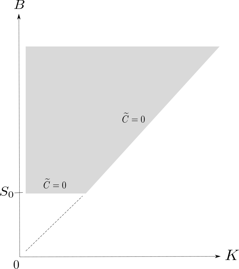
Figure 4.1. PIDE Domain and Boundaries

The initial condition (4.2) is the payoff obtained at maturity. Condition (4.3) expresses the fact that the option gets knocked out before being in-the-money if $K=B$, while (4.4) says the option gets knocked out immediately at inception if $S_{0}=B$.

Remark.

We note that in the models we will consider, no boundary condition needs to be specified at $K=0$, since the coefficients of the $K$-derivatives vanish sufficiently fast as $K\rightarrow 0$. This is the case, e.g., if $\sigma_{|S,M}^{2}$ and its $B$-derivative are bounded when $K\rightarrow 0$.

In fact, a boundary condition at $K=0$ could be derived by differentiating (2.9) twice,

$$\frac{\partial^{2}\widetilde{C}\mathopen{}\mathclose{{}\left(0,B,T}\right)}{\partial K^{2}} = D\mathopen{}\mathclose{{}\left(T}\right)Q\mathopen{}\mathclose{{}\left(T}\right)\int_{S_{0}}^{B}\phi\mathopen{}\mathclose{{}\left(0,y,T}\right){\,\rm d}y=D\mathopen{}\mathclose{{}\left(T}\right)Q\mathopen{}\mathclose{{}\left(T}\right)\mathbb{Q}\mathopen{}\mathclose{{}\left(S_{0}<M_{T}<B\mid S_{T}=0}\right)\psi(0,T),$$

where $\psi(0,T)$ is the density of $S_{T}$ at 0. The latter is equal to zero since the density of the spot at zero is zero under the log-spot model in (2.1). Linearity conditions, also known as “Zero Gamma” for spot PDEs, are commonly used in finance and particularly useful for exotic contracts. They usually lead to stable numerical schemes (see Windcliff [23]).

We also note that

(4.5) $$\frac{\partial^{2}\widetilde{C}\mathopen{}\mathclose{{}\left(B,B,T}\right)}{\partial K^{2}}=D\mathopen{}\mathclose{{}\left(T}\right)Q\mathopen{}\mathclose{{}\left(T}\right)\mathbb{Q}\mathopen{}\mathclose{{}\left(S_{0}<M_{T}<B\mid S_{T}=B}\right)\psi(B,T)=0,$$

because if the spot is equal to $B$ at $T$, then the probability that the running maximum is smaller than $B$ is zero. While we will use the Dirichlet condition on the boundary $K=B$ for computations, (4.5) allows us to express the third order cross derivative in the second line of (4.1) by a third order derivative only with respect to $K$. Indeed,

$$0=\frac{{\rm d}}{{\rm d}B}\mathopen{}\mathclose{{}\left(\frac{\partial^{2}\widetilde{C}\mathopen{}\mathclose{{}\left(B,B,T}\right)}{\partial K^{2}}}\right)=\frac{\partial^{3}\widetilde{C}\mathopen{}\mathclose{{}\left(B,B,T}\right)}{\partial K^{3}}+\frac{\partial^{3}\widetilde{C}\mathopen{}\mathclose{{}\left(B,B,T}\right)}{\partial K^{2}\partial B},$$

leading to

(4.6) $$\frac{\partial^{3}\widetilde{C}\mathopen{}\mathclose{{}\left(B,B,T}\right)}{\partial K^{3}}=-\frac{\partial^{3}\widetilde{C}\mathopen{}\mathclose{{}\left(B,B,T}\right)}{\partial K^{2}\partial B}.$$

The domain sketched in Fig. 4.1 is unbounded for large $B$. We denote $B_{Max}$ the maximum value of barrier levels we will consider in the numerical solution. Note that because of the structure of (4.1), no boundary condition is needed for $B=B_{Max}$.

4.2. Finite Difference Approximation

We define a uniform mesh which contains $M+1$ time points, $N+1$ spatial points in the strike and $P+1$ in the barrier variable, leading to the following definition of the step sizes:

$$\begin{array}[]{lclll}K_{i}&=&i\Delta_{K},&\Delta_{K}=\frac{B_{Max}-S_{0}}{N+1},&i\in\mathopen{}\mathclose{{}\left\llbracket 0,N}\right\rrbracket,\\ B_{j}&=&S_{0}+j\Delta_{B},&\Delta_{B}=\frac{B_{Max}-S_{0}}{P+1},&j\in\mathopen{}\mathclose{{}\left\llbracket 0,P}\right\rrbracket,\\ T_{m}&=&m\Delta_{T},&\Delta_{T}=\frac{T_{Max}}{M+1},&m\in\mathopen{}\mathclose{{}\left\llbracket 0,M}\right\rrbracket.\end{array}$$

For simplicity, we impose $\Delta_{K}=\Delta_{B}$. This will ensure that for any $B_{j}$, the corresponding mesh line will contain at least all $(B_{u},B_{j})$ for all $u$ smaller than $j$, which is useful for the following algorithm.

We can identify an interesting property of (4.1), especially visible with the substitution (4.6), in order to approximate the solution inductively on a discrete lattice. At $B=S_{0}$, the solution is known to be uniformly zero over the strike and time variable. Assume now an approximate solution is known up to a certain $B$. Moving from $B$ to $B+\Delta_{B}$, and approximating the integral by a quadrature rule, gives a PDE in time and strike at level $B+\Delta_{B}$, which can be solved by finite differences. From now on, we will refer to the PDE at a given barrier level $B_{j}$ as a “PDE layer”. We can then solve the PIDE for each layer at points $B_{j}$ from $S_{0}$ to $B_{Max}$.

We denote the discrete solution vector in such a layer by

$$\mathbf{u}_{.,j}^{m}=\begin{bmatrix}\widetilde{C}\mathopen{}\mathclose{{}\left(K_{0},B_{j},T_{m}}\right),\ldots,\widetilde{C}\mathopen{}\mathclose{{}\left(B_{j},B_{j},T_{m}}\right)\end{bmatrix}^{\prime}$$

of size $n_{j}=\frac{B_{j}-K_{0}}{\Delta_{K}}+1$, where ^′ denotes the transpose. We also denote by $\mathbf{I}_{n}$ the identity matrix of size $n\times n$.

Derivatives

Derivatives are approximated by centered finite differences at each space point except at $K=0$ and $K=B_{j}$, where they are computed, respectively, forward and backward. For the time being, the boundary conditions are not taken into account. We assume equally spaced points and define two operators as follows:

$$\delta_{K}\mathbf{u}_{i,j}^{m} = \frac{\mathbf{u}_{i+1,j}^{m}-\mathbf{u}_{i-1,j}^{m}}{2\Delta_{K}},$$

(4.8) $$\delta_{KK}\mathbf{u}_{i,j}^{m} = \frac{\mathbf{u}_{i+1,j}^{m}-2\mathbf{u}_{i,j}^{m}+\mathbf{u}_{i-1,j}^{m}}{\Delta_{K}^{2}}.$$

The usual matrix derivative operator can be defined for both the first and second order derivative:

$$\mathbf{D}=\frac{1}{\Delta_{K}}\begin{bmatrix}-1&1&0&...&0\\ -\frac{1}{2}&0&\frac{1}{2}&\ddots&\vdots\\ 0&\ddots&\ddots&\ddots&0\\ \vdots&\ddots&-\frac{1}{2}&0&\frac{1}{2}\\ 0&...&0&-1&1\end{bmatrix},\quad\mathbf{D_{2}}=\frac{1}{\Delta_{K}^{2}}\begin{bmatrix}1&-2&1&0&...&0\\ 1&-2&1&0&\mathopen{}\mathclose{{}\left(0}\right)&\vdots\\ 0&\ddots&\ddots&\ddots&\ddots&\vdots\\ \vdots&\ddots&\ddots&\ddots&\ddots&0\\ \vdots&\mathopen{}\mathclose{{}\left(0}\right)&0&1&-2&1\\ 0&...&0&1&-2&1\end{bmatrix}.$$

We also define the forward time difference operator

$$\delta_{T}\mathbf{u}_{i,j}^{m}=\frac{\mathbf{u}_{i,j}^{m+1}-\mathbf{u}_{i,j}^{m}}{\Delta T}.$$

Integral

The integral term will be computed using the trapezoidal quadrature rule. This yields an order two consistent approximation. The term of interest is

$$F\mathopen{}\mathclose{{}\left(K_{i},B_{j},T_{m}}\right) = \int_{S_{0}\lor K}^{B_{j}}-\frac{1}{2}K_{i}^{2}\frac{\partial^{2}\widetilde{C}\mathopen{}\mathclose{{}\left(K_{i},b,T_{m}}\right)}{\partial K^{2}}\frac{\partial\sigma_{|S,M}^{2}\mathopen{}\mathclose{{}\left(K_{i},b,T_{m}}\right)}{\partial b}{\,\rm d}b.$$

Let us assume that we know an approximation to the solution of the PIDE for the discrete set of barriers $\mathopen{}\mathclose{{}\left(B_{n}}\right)_{n<j}$. We also know that, when the barrier is at the spot level, the integrand is zero. Hence,

$$F\mathopen{}\mathclose{{}\left(K_{i},B_{j},T_{m}}\right) = -\,\,\sum_{n=1}^{j-1}\mathopen{}\mathclose{{}\left(\frac{1}{2}K_{i}^{2}\frac{\partial^{2}\widetilde{C}\mathopen{}\mathclose{{}\left(K_{i},B_{n},T_{m}}\right)}{\partial K^{2}}\frac{\partial\sigma_{|S,M}^{2}\mathopen{}\mathclose{{}\left(K_{i},B_{n},T_{m}}\right)}{\partial B}\Delta_{B}}\right)$$

$$-\,\,\frac{1}{4}K_{i}^{2}\frac{\partial^{2}\widetilde{C}\mathopen{}\mathclose{{}\left(K_{i},B_{j},T_{m}}\right)}{\partial K^{2}}\frac{\partial\sigma_{|S,M}^{2}\mathopen{}\mathclose{{}\left(K_{i},B_{j},T_{m}}\right)}{\partial B}\Delta_{B}$$

$$+\,\,\mathcal{O}\mathopen{}\mathclose{{}\left(\Delta_{B}^{2}}\right).$$

The sum in the first line can be computed for all $K_{i}$ and $T_{m}$ in a forward induction over $j$, as the solution is known for all the barrier levels involved. This sum is then treated as a source function for the PDE layer of level $B_{j}$. We define a vector

$$\mathbf{f}_{.,j}^{m}=\mathopen{}\mathclose{{}\left[\begin{array}[]{c}-\sum_{n=1}^{j-1}\mathopen{}\mathclose{{}\left(\frac{1}{2}K_{i}^{2}\delta_{KK}\mathbf{u}_{i,n}^{m}\frac{\partial\sigma_{|S,M}^{2}\mathopen{}\mathclose{{}\left(K_{i},B_{n},T_{m}}\right)}{\partial B}\Delta_{B}}\right)\end{array}}\right]_{i=0,1,...,n_{j}}.$$

The remaining term in (4.2) gives a small correction to the diffusion at $B_{j}$ and we can incorporate it in the discretisation of the corresponding diffusive term of (4.1).

Boundary Derivative Term

To approximate the “boundary derivative” at $(B,B,T)$ in (4.1), we use (4.6) and a first order approximation to the third derivative with discretisation matrix written as

$$\mathbf{\Phi}=\frac{1}{\Delta_{K}^{3}}\begin{bmatrix}0&\ldots&0&\text{0}&-1&3&-3&1\\ \vdots&\mathopen{}\mathclose{{}\left(0}\right)&\vdots&\vdots&\vdots&\vdots&\vdots&\vdots\\ 0&\ldots&0&0&-1&3&-3&1\end{bmatrix}.$$

As this term is present in the discretised equation for all interior mesh points, this reduces the consistency order in $\Delta_{K}$ of the overall scheme to one. We found higher order finite differences to be unstable.

Remark.

A second order accurate stable scheme can be obtained by using (2.11) to replace the third order derivative at the boundary by the density, which can be found by solving the Kolmogorov forward equation (2.6) numerically.

PIDE in Terms of Matrix Operations

If we take into account the finite difference approximations and quadrature rule for the integral, it is now possible to give a discretised PIDE, for a given triplet $\mathopen{}\mathclose{{}\left(i,j,m}\right)\in\mathopen{}\mathclose{{}\left\llbracket 0,N}\right\rrbracket\times\mathopen{}\mathclose{{}\left\llbracket 0,M}\right\rrbracket\times\mathopen{}\mathclose{{}\left\llbracket 0,P}\right\rrbracket$ by

$$\delta_{T}\mathbf{u}_{i,j}^{m}+\mathopen{}\mathclose{{}\left(r\mathopen{}\mathclose{{}\left(T_{m}}\right)-q\mathopen{}\mathclose{{}\left(T_{m}}\right)}\right)K_{i}\delta_{K}\mathbf{u}_{i,j}^{m}-\frac{1}{2}\mathopen{}\mathclose{{}\left(\sigma_{|S,M}^{2}\mathopen{}\mathclose{{}\left(K_{i},B_{j},T_{m}}\right)-\frac{1}{2}\frac{\partial\sigma_{|S,M}^{2}\mathopen{}\mathclose{{}\left(K_{i},B_{j},T_{m}}\right)}{\partial B}\Delta_{B}}\right)K_{i}^{2}\delta_{KK}\mathbf{u}_{i,j}^{m}$$

(4.10) $$+\frac{1}{2}\sigma_{|S,M}^{2}\mathopen{}\mathclose{{}\left(B_{j},B_{j},T_{m}}\right)B_{j}^{2}\mathopen{}\mathclose{{}\left(B_{j}-K}\right)^{+}\delta_{KKB}^{-}\mathbf{u}_{n_{j},j}^{m} =$$

$$-\sum_{n=1}^{j-1}\frac{1}{2}K_{i}^{2}\delta_{KK}\mathbf{u}_{i,j}^{m}\frac{\partial\sigma_{|S,M}^{2}\mathopen{}\mathclose{{}\left(K_{i},B_{n},T_{m}}\right)}{\partial B}\Delta_{B},$$

and specify the coefficient matrices

$$\mathbf{A}_{.,j}^{m} = \mathopen{}\mathclose{{}\left(r\mathopen{}\mathclose{{}\left(T_{m}}\right)-q\mathopen{}\mathclose{{}\left(T_{m}}\right)}\right)\text{diag}\mathopen{}\mathclose{{}\left(K_{0},...,K_{n_{j}}}\right),$$

$$\mathbf{B}_{.,j}^{m} = -\frac{1}{2}\text{diag}\mathopen{}\mathclose{{}\left(\mathopen{}\mathclose{{}\left(\sigma_{|S,M}^{2}\mathopen{}\mathclose{{}\left(K_{i},B_{j},T_{m}}\right)K_{i}^{2}-\frac{1}{2}K_{i}^{2}\frac{\partial\sigma_{|S,M}^{2}\mathopen{}\mathclose{{}\left(K_{i},B_{j},T_{m}}\right)}{\partial B}\Delta_{B}}\right)_{i\in\mathopen{}\mathclose{{}\left\llbracket 0,n_{j}}\right\rrbracket}}\right),$$

$$\mathbf{C}_{.,j}^{m} = -\frac{1}{2}\text{diag}\mathopen{}\mathclose{{}\left(\mathopen{}\mathclose{{}\left(\sigma_{|S,M}^{2}\mathopen{}\mathclose{{}\left(B_{j},B_{j},T_{m}}\right)B_{j}^{2}\mathopen{}\mathclose{{}\left(B_{j}-K_{i}}\right)^{+}}\right)_{i\in\mathopen{}\mathclose{{}\left\llbracket 0,n_{j}}\right\rrbracket}}\right).$$

Remark.

We can also approximate $\mathbf{B}_{.,j}^{m}$ further by Taylor expansion,

$$\mathbf{B}_{.,j}^{m}=-\frac{1}{2}\text{diag}\mathopen{}\mathclose{{}\left(\mathopen{}\mathclose{{}\left(\sigma_{|S,M}^{2}\mathopen{}\mathclose{{}\left(K_{i},B_{j}-\frac{\Delta_{B}}{2},T_{m}}\right)K_{i}^{2}}\right)_{i\in\mathopen{}\mathclose{{}\left\llbracket 0,n_{j}}\right\rrbracket}}\right)+\mathcal{O}\mathopen{}\mathclose{{}\left(\Delta_{B}^{2}}\right),$$

which has a negative sign irrespective of the mesh size and does not alter the convergence order.

Under forward Euler time stepping, the complete scheme can be more compactly written as

$$\frac{\mathbf{u}_{.,j}^{m+1}-\mathbf{u}_{.,j}^{m}}{\Delta T}+\mathbf{L}_{.,j}^{m}\mathbf{u}_{.,j}^{m} = \mathbf{f}_{.,j}^{m},$$

$$\mathbf{\mathbf{L}}_{.,j}^{m} = \mathbf{A}_{.,j}^{m}\mathbf{D}+\mathbf{B}_{.,j}^{m}\mathbf{D_{2}}+\mathbf{C}_{.,j}^{m}\mathbf{\Phi}.$$

Under $\theta$-time-stepping, the scheme becomes

$$\mathopen{}\mathclose{{}\left(\mathbf{I}_{n_{j}}+\theta\Delta_{T}\mathbf{L}_{.,j}^{m+1}}\right)\mathbf{u}_{.,j}^{m+1}=\mathopen{}\mathclose{{}\left(\mathbf{I}_{n_{j}}-\mathopen{}\mathclose{{}\left(1-\theta}\right)\Delta_{T}\mathbf{L}_{.,j}^{m}}\right)\mathbf{u}_{.,j}^{m}+\theta\Delta_{T}\mathbf{f}_{.,j}^{m+1}+\mathopen{}\mathclose{{}\left(1-\theta}\right)\Delta_{T}\mathbf{f}_{.,j}^{m}.$$

This includes the second-order accurate Crank-Nicolson scheme for $\theta=0.5$, which is used for our numerical computations.

This section shows that we can adapt the classical tools of finite difference methods in order to solve this PIDE. Each of the layers being a one-dimensional PDE, it is solved by successive roll-forward performed by a Gaussian elimination. Although the Thomas algorithm cannot be applied directly since $\mathbf{L}_{.,j}^{m}$ is not tri-diagonal (even after applying the necessary boundary conditions), a sparse Gaussian elimination will still be $\mathcal{O}\mathopen{}\mathclose{{}\left(n}\right)$ as the dense sub-matrix has a fixed number of columns.

Solution Algorithm

We conclude with a summary of a possible algorithm to solve the PIDE numerically:

Algorithm 1 PIDE Discretisation

$\mathbf{u}_{.,j}^{0}$ = $\mathopen{}\mathclose{{}\left(\mathopen{}\mathclose{{}\left(S_{0}-K_{i}}\right)^{+}\mathbf{1}_{S_{0}<B_{j}}}\right)_{i\in\mathopen{}\mathclose{{}\left\llbracket 0,N}\right\rrbracket}$

$\mathbf{u}_{.,0}^{m}=0$

$\mathbf{f}_{.,0}^{m}=0$

  for  ( $j=0\,;\,j\leq P\,;\,j++$)  do

      solve $B_{j}-$layer PDE for $\mathopen{}\mathclose{{}\left(\mathbf{u}_{.,j}^{m}}\right)_{m\in\mathopen{}\mathclose{{}\left\llbracket 0,M}\right\rrbracket}$:

$$\mathopen{}\mathclose{{}\left(\mathbf{I}_{n_{j}}+\theta\Delta_{T}\mathbf{L}_{.,j}^{m+1}}\right)\mathbf{u}_{.,j}^{m+1}=\mathopen{}\mathclose{{}\left(\mathbf{I}_{n_{j}}-\mathopen{}\mathclose{{}\left(1-\theta}\right)\Delta_{T}\mathbf{L}_{.,j}^{m}}\right)\mathbf{u}_{.,j}^{m}+\theta\Delta_{T}\mathbf{f}_{.,j}^{m+1}+\mathopen{}\mathclose{{}\left(1-\theta}\right)\Delta_{T}\mathbf{f}_{.,j}^{m}$$

      compute $\mathbf{f}_{.,j+1}^{m}$ from $\mathbf{f}_{.,j}^{m}$ and $\mathbf{u}_{.,j}^{m}$ (for $j<P$)

  end for

5. Numerical Results

5.1. Pricing Under the Mimicking Brunick-Shreve Model

For validation purposes of the forward equation, we will use a numerical solution of the backward pricing PDE in the Brunick-Shreve model. The backward PDE gives the price over a range of $S$ and $M$ and $t$, for fixed $K$, $B$ and $T$.

Augmented State Feynman-Kac PDE

Recall that the spot diffusion of the underlying under $\mathbb{Q}$ is

(5.1) $$\cfrac{dS_{t}}{S_{t}}=\mathopen{}\mathclose{{}\left(r\mathopen{}\mathclose{{}\left(t}\right)-q\mathopen{}\mathclose{{}\left(t}\right)}\right)\,dt+\sigma\mathopen{}\mathclose{{}\left(S_{t},M_{t},t}\right)\,dW_{t}.\$$

We note that the spot process is not Markovian anymore due to the dependence of the volatility on the running maximum. Hence, we cannot use the standard one dimensional Feynman-Kac PDE with Dirichlet boundary condition, but need to augment the state space even for barrier options (as well as European options). Assume that strike $K$, barrier $B$ and maturity $T$ are all fixed. Then, following identical steps to the derivation by Shreve [21] in the Black-Scholes case, we get the following (see Appendix A).

Proposition 5.

Under a Brunick-Shreve model (5.1), the up-and-out call price $C$ defined in the region $\small{\Omega_{B}=\{(x,y):0<x<y,S_{0}<y<B\}}$ is the solution to the following initial boundary value problem:

(5.2) $$\frac{\partial C}{\partial t}+\mathopen{}\mathclose{{}\left(r\mathopen{}\mathclose{{}\left(t}\right)-q\mathopen{}\mathclose{{}\left(t}\right)}\right)x\frac{\partial C}{\partial x}+\frac{1}{2}x^{2}\sigma^{2}\mathopen{}\mathclose{{}\left(x,y,t}\right)\frac{\partial^{2}C}{\partial x^{2}}-r\mathopen{}\mathclose{{}\left(t}\right)C=0,\, (x,y)\in\Omega_{B},\;0<t<T,$$

$$C\mathopen{}\mathclose{{}\left(0,y,t}\right)=0, t\leq T,$$

$$C\mathopen{}\mathclose{{}\left(x,y,T}\right)=\mathopen{}\mathclose{{}\left(x-K}\right)^{+}\mathbf{1}_{y<B}, y>S_{0},$$

$$\mathopen{}\mathclose{{}\left.\frac{\partial C\mathopen{}\mathclose{{}\left(x,y,t}\right)}{\partial y}}\right\rfloor_{x=y}=0, y>S_{0},$$

$$C\mathopen{}\mathclose{{}\left(x,B,t}\right)=0, x>0,\,t\leq T.$$

Finite Difference Approximation

We briefly explain the numerical solution of (5.2).

We first notice that (5.2) is a classical Black-Scholes PDE (where the volatility is a function of $S$, a “parameter” $M$, and $t$), and derivatives with respect to $y$ only enter via the Neumann boundary condition (on the diagonal $x=y$). This means that for a fixed $y$, we have to solve a Black-Scholes type PDE on $\mathopen{}\mathclose{{}\left[0,y}\right]\ \times\{y\}$. From now on, the one-dimensional PDE for a given level of $y$ will be referred to as a “PDE layer”.

If $y=B$, then $C\mathopen{}\mathclose{{}\left(x,y,t}\right)=0$ for all $x$. We can then use the Neumann boundary condition to bootstrap backwards in $y$ from $B$ to $S_{0}$. To illustrate the idea, consider now $y=B-\Delta_{y}$ for a mesh size $\Delta_{y}$, then

$$\mathopen{}\mathclose{{}\left.\frac{\partial C\mathopen{}\mathclose{{}\left(x,y,t}\right)}{\partial y}}\right\rfloor_{x=y}=\frac{C\mathopen{}\mathclose{{}\left(y,y+\Delta_{y},t}\right)-C\mathopen{}\mathclose{{}\left(y,y,t}\right)}{\Delta y}+\mathcal{O}\mathopen{}\mathclose{{}\left(\Delta_{y}}\right)=0\implies C\mathopen{}\mathclose{{}\left(y,y,t}\right)=C\mathopen{}\mathclose{{}\left(y,y+\Delta_{y},t}\right)+\mathcal{O}\mathopen{}\mathclose{{}\left(\Delta_{y}^{2}}\right).$$

We can build the next PDE layer at $y$ using an approximate Dirichlet boundary condition at $x=y$, $C\mathopen{}\mathclose{{}\left(y,y,t}\right)\approx C\mathopen{}\mathclose{{}\left(y,y+\Delta_{y},t}\right)$ (here, 0). Subsequent PDE layers can be constructed similarly by backward reasoning. We will describe a higher-order version below. The solution in each layer will then depend on layers with greater $y$ via this boundary condition. The premium value is retrieved from $C\mathopen{}\mathclose{{}\left(S_{0},S_{0},0}\right)$.

We now describe the construction of meshes of the form $(x_{j}(y),y)_{j=1,\ldots,N_{x}(y)}$ for layer $y$, as well as of the spacing of points in the $y$-direction. The best accuracy was achieved numerically with a refined running maximum grid close to $S_{0}$ and, for each $y$, a uniformly spaced spot grid (except for nodes close to the diagonal, as detailed below).

Denote by $\Delta_{y}$ a desired target mesh width. Then for the $y$-mesh we choose $N_{y}=\mathopen{}\mathclose{{}\left\lceil\frac{B-S_{0}}{\Delta_{y}}}\right\rceil$ points with an exponential grading as defined in [22], so that $\forall\,i$$\in\mathopen{}\mathclose{{}\left\llbracket 0,N_{y}}\right\rrbracket$:

$$y_{i} = \mathopen{}\mathclose{{}\left(S_{0}-\theta}\right)+\theta\,\exp\mathopen{}\mathclose{{}\left(\lambda z_{i}}\right),$$

$$\lambda = 2,$$

$$\theta = \frac{B-S_{0}}{e^{\lambda}-1},$$

$$z_{i} = \frac{i}{\mathopen{}\mathclose{{}\left(N_{y}+1}\right)}.$$

The construction of the mesh, illustrated in Figure 5.1, ensures that $y_{i}$ lies on the grid of the PDE layer of levels $y_{i+1}$ and $y_{i+2}$, and hence no interpolation is needed to retrieve the boundary condition for the next PDE layer as described in the next paragraph.

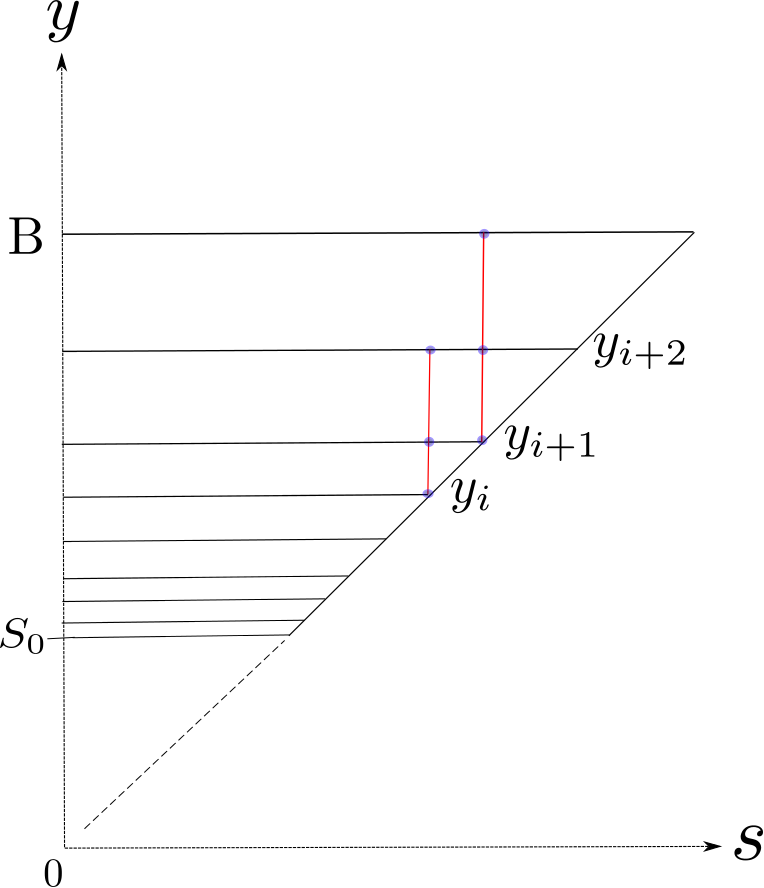
Figure 5.1. Mesh construction for backward equation. The spot grid is recomputed for every PDE layer to be $(x_{j}(y_{i}),y_{i})$, where $x_{j}=j\Delta_{x}$, $j<N_{x}-2$, $x_{N_{x}-j}=y_{i-j}$, $j\in\{0,1,2\}$, $\Delta_{x}=y_{i-2}/(N_{x}-2)$ and $N_{x}=\mathopen{}\mathclose{{}\left\lceil y_{i}/\Delta_{y}}\right\rceil$ to keep the spacing approximately constant.

In order to increase accuracy from the numerical boundary condition described at the start of this section, we use second order Taylor expansion in $y$-direction instead of a simple backward finite difference for all $y_{i}$ with $i<N_{y}-1$. The bootstrap idea stays the same. Indeed, write $c\mathopen{}\mathclose{{}\left(y}\right)=c\mathopen{}\mathclose{{}\left(y_{i},y,t}\right)$ where $y_{i}$ is a certain given level of the $y$-discretisation and $c^{\prime}\mathopen{}\mathclose{{}\left(y}\right)=\frac{\partial c\mathopen{}\mathclose{{}\left(y_{i},y,t}\right)}{\partial y}$. We consider a Taylor expansion around $y=y_{i}$: $c\mathopen{}\mathclose{{}\left(y}\right)=c\mathopen{}\mathclose{{}\left(y_{i}}\right)+\frac{1}{2}\mathopen{}\mathclose{{}\left(y-y_{i}}\right)^{2}c^{\prime\prime}\mathopen{}\mathclose{{}\left(y_{i}}\right)+o\mathopen{}\mathclose{{}\left((y-y_{i})^{2}}\right)$ (as $c^{\prime}\mathopen{}\mathclose{{}\left(y_{i}}\right)=0$ by the boundary condition). Using this at points $y_{i+1}$ and $y_{i+2}$, we get $c\mathopen{}\mathclose{{}\left(y_{i}}\right)=c\mathopen{}\mathclose{{}\left(y_{i+2}}\right)+\frac{\mathopen{}\mathclose{{}\left(y_{i+2}-y_{i}}\right)^{2}}{\mathopen{}\mathclose{{}\left(y_{i+2}-y_{i}}\right)^{2}-\mathopen{}\mathclose{{}\left(y_{i+1}-y_{i}}\right)^{2}}\mathopen{}\mathclose{{}\left(c\mathopen{}\mathclose{{}\left(y_{i+1}}\right)-c\mathopen{}\mathclose{{}\left(y_{i+2}}\right)}\right)$. This is then used as a boundary value at $y_{i}$. The first layer at $N_{y}-1$ is treated with a first order backward difference as described previously.

5.2. Numerical Validation

Our numerical validation consists in pricing a set of up-and-out call options for different strikes, maturities and barriers with:

1. the Forward PIDE (4.1) and one numerical solution for the whole set of deal parameters;

2. the Backward Feynman-Kac PDE (5.2) and as many solutions as triplets of deal parameters.

The goal is to make them match with about one basis point tolerance.

The Brunick-Shreve volatility is generated with an SVI parametrisation in both barrier and strike dimension (details can be found in [15]) defined as

(5.3) $$\sigma\mathopen{}\mathclose{{}\left(x,y,t}\right) = \frac{1}{2}\mathopen{}\mathclose{{}\left(\sigma_{SVI}\mathopen{}\mathclose{{}\left(\log\mathopen{}\mathclose{{}\left(\frac{x}{S_{0}}}\right),t+1}\right)+\sigma_{SVI}\mathopen{}\mathclose{{}\left(\log\mathopen{}\mathclose{{}\left(\frac{y}{S_{0}}}\right),t+1}\right)}\right),$$

$$\sigma_{SVI}\mathopen{}\mathclose{{}\left(k,t}\right) = \sqrt{a+b\mathopen{}\mathclose{{}\left(\rho\mathopen{}\mathclose{{}\left(k-m}\right)+\sqrt{\mathopen{}\mathclose{{}\left(k-m}\right)^{2}+\sigma^{2}}}\right)}.$$

The Brunick-Shreve volatility surface has a shape as in Figure 5.2.

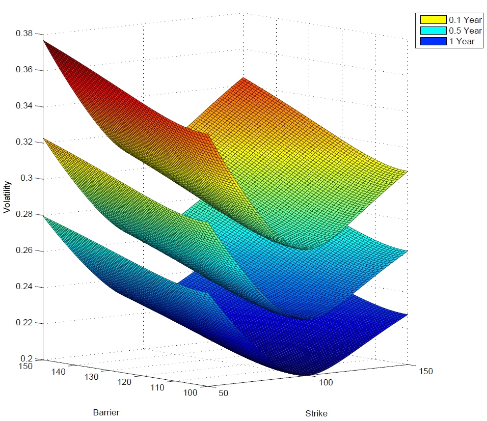
Figure 5.2. Assumed Brunick-Shreve volatility surface as per (5.3), where $a=0.04,b=0.2,\sigma=0.2,\rho=m=0$, and $T\in\{0.1,0.5,1\}$.

The spot is $S_{0}=100$, the risk-free rate is $r=0.1$ and the dividend yield is $q=0.05$.

We use the numerical schemes as described in 4.2 and 5.1 for the PIDE and PDE solution, respectively, with Crank-Nicolson time stepping. The discretisation parameters are $N=P=N_{y}=1000$ space steps (with $N_{x}$ adjusted as described) and $M=1000$ time steps.

We compare prices for $\mathopen{}\mathclose{{}\left(K,B,T}\right)$ covering the set $\mathopen{}\mathclose{{}\left[0,120}\right]\times\mathopen{}\mathclose{{}\left[100,120}\right]\times\mathopen{}\mathclose{{}\left\{1}\right\}$ with 120 points in strike and 40 points in barrier levels, see Table 1. The error is computed as the relative error if the net present value (NPV) is above one and as absolute error otherwise.

Average Difference	Maximum Difference
4.6e-5	3.5e-4

Table 1. Difference between forward and backward solutions over strikes between 0 and 120, and up-and-out barriers between 100 and 120, all for maturity 1.

We can analyse more precisely the behaviour for a few barrier levels. For example, Figure 5.3 shows the difference as a function of strike. The associated values for a barrier fixed at 120 are in Table 2.

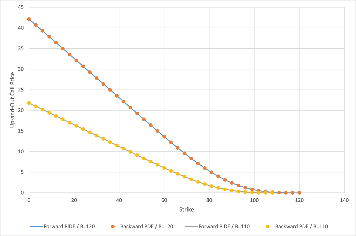
Figure 5.3. Forward PIDE vs Backward PDE:
up-and-out call option prices with Brunick-Shreve volatility, $S=100$ and $T=1$.

Strike	Forward	Backward	Rel.
	PIDE	PDE	Diff.
0	42.1486	42.1486	1e-06
9	37.8567	37.8568	1e-06
18	33.5649	33.5650	2e-06
27	29.2731	29.2732	2e-06
36	24.9815	24.9815	3e-06
45	20.6928	20.6929	3e-06
54	16.4263	16.4264	2e-06
63	12.2536	12.2535	5e-06
72	8.3438	8.3436	2e-05
81	4.9680	4.9677	6e-05
90	2.4170	2.4168	9e-05
99	0.8472	0.8472	9e-07
108	0.1546	0.1547	1e-04
117	0.0023	0.0023	8e-05
120	0.0000	0.0000	0

Table 2. Results and relative errors for different strikes; barrier = 120, forward = 105.13.

The results match with the desired accuracy.

6. Conclusions

In this paper, we provided a new and numerically effective way to work with observed barrier option prices to determine the Brunick-Shreve Markovian projection of a stochastic variance of a semi-martingale $S$ with running maximum $M$ onto $\mathopen{}\mathclose{{}\left(S_{t},M_{t}}\right)$. The present Dupire-type formula, which provides similar advantages (and disadvantages) as the standard Dupire approach for vanillas, was then re-arranged to obtain a forward PIDE, which is convenient to control the numerical stability of best fit algorithms [8]. There is a well-known literature on the calibration of vanilla options through Markovian projection for LSV models (see Guyon and Labordère [17] and Ren, Madan and Quian [20]). We believe that extending these methods combined with the Forward PIDE we presented in this paper will lead to novel calibration algorithms for barrier options.

Acknowledgements

The authors thank Marek Musiela from the Oxford-Man Institute, Alan Bain and Simon McNamara from BNP Paribas London as well as an anonymous referee for their insightful comments.

Appendix A Derivation of the Kolmogorov Forward and Backward Equations

In this section, we derive the forward and backward Kolmogorov equations for a model of the type

$$\cfrac{dS_{t}}{S_{t}} = (r\mathopen{}\mathclose{{}\left(t}\right)-q\mathopen{}\mathclose{{}\left(t}\right))\,dt+\sigma(S_{t},M_{t},t)\,dW_{t},$$

$$M_{t} = \underset{0\leq u\leq t}{\max}S_{u}$$

and under Assumption 1.

The Backward Equation (Derivation of Proposition 5)

We first note that the up-and-out call is a traded contract. As a consequence, the discounted price process $D(t){C}_{t}$ is a martingale under the risk-neutral measure $\mathbb{Q}$. Hence

$$D(t)C_{t}=\mathbb{E^{\mathbb{Q}}}\mathopen{}\mathclose{{}\left[D(T)\mathopen{}\mathclose{{}\left({S}_{T}-K}\right)^{+}\mathbf{1}_{{M}_{T}<B}\mid\mathcal{F}_{t}}\right]\qquad\;0\leq t\leq T.$$

Furthermore, as $\mathopen{}\mathclose{{}\left(S_{t},M_{t}}\right)$ is a Markovian vector, there exists a function $v$ such that

$$D(t)v(x,y,t)=\mathbb{E^{\mathbb{Q}}}\mathopen{}\mathclose{{}\left[D(T)\mathopen{}\mathclose{{}\left({S}_{T}-K}\right)^{+}\mathbf{1}_{{M}_{T}<B}\mid S_{t}=x,\,M_{t}=y}\right]\qquad\forall(x,y)\in\Omega_{B},\;0\leq t\leq T.$$

We assume that $v$ is smooth and belongs to the space $C^{2,1,1}(\Omega_{B}\times\mathbb{R}^{+})$. Now write

$$C_{t}=v(S_{t},M_{t},t).$$

By the Itô-Doeblin lemma and recalling that the running maximum process $M$ has finite variation, zero quadratic variation and zero cross-variation with $S$,

$$d(D(t)C_{t}) = -r\mathopen{}\mathclose{{}\left(t}\right)D(t)C_{t}\,dt+D(t)\mathopen{}\mathclose{{}\left[\frac{\partial v}{\partial t}\,dt+\frac{\partial v}{\partial x}\,dS_{t}+\frac{\partial v}{\partial y}\,dM_{t}+\frac{1}{2}\frac{\partial^{2}v}{\partial x^{2}}\,d[S]_{t}}\right].$$

The process $D\mathopen{}\mathclose{{}\left(t}\right){C}_{t}$ is a martingale if and only if

(A.1) $$\frac{\partial v}{\partial t}-r\mathopen{}\mathclose{{}\left(t}\right)v+(r\mathopen{}\mathclose{{}\left(t}\right)-q\mathopen{}\mathclose{{}\left(t}\right))x\frac{\partial v}{\partial x}+\frac{1}{2}\sigma^{2}x^{2}\frac{\partial^{2}v}{\partial x^{2}} = 0,\quad(x,y)\in\Omega_{B},\;0<t<T,$$

$$\mathopen{}\mathclose{{}\left.\frac{\partial v}{\partial y}}\right\rfloor_{x=y} = 0,\quad y>S_{0}.$$

This gives the desired backward PDE. We note that the boundary condition is equivalent to

(A.2) $$\frac{{\rm d}v(y,y,t)}{{\,\rm d}y}=\mathopen{}\mathclose{{}\left.\frac{\partial v(x,y,t)}{\partial x}}\right\rfloor_{x=y}.$$

The Forward Equation (Derivation of Proposition 1)

We assume as before that the joint density function $\phi$ of the process $(S_{t},M_{t})$ exists and belongs to the space $C^{2,1,1}(\Omega\times\mathbb{R}^{+})$.

Let $h\in C^{2,1}\mathopen{}\mathclose{{}\left(\Omega}\right)$ be a test function of two (spatial) variables. We also assume that $h$ and its derivatives vanish for $x=0$. We denote $\mu\mathopen{}\mathclose{{}\left(t}\right)=r\mathopen{}\mathclose{{}\left(t}\right)-q\mathopen{}\mathclose{{}\left(t}\right)$.

We apply the Itô-Doeblin lemma and get:

$$h\mathopen{}\mathclose{{}\left(S_{t},M_{t}}\right) = h\mathopen{}\mathclose{{}\left(S_{0},M_{0}}\right)$$

$$+\int_{0}^{t}\mathopen{}\mathclose{{}\left[\mu\mathopen{}\mathclose{{}\left(u}\right)S_{u}\frac{\partial h\mathopen{}\mathclose{{}\left(S_{u},M_{u}}\right)}{\partial x}+\frac{1}{2}\sigma^{2}\mathopen{}\mathclose{{}\left(S_{u},M_{u},u}\right)S_{u}^{2}\frac{\partial^{2}h\mathopen{}\mathclose{{}\left(S_{u},M_{u}}\right)}{\partial x^{2}}}\right]{\,\rm d}u$$

$$+\int_{0}^{t}\sigma\mathopen{}\mathclose{{}\left(S_{u},M_{u},u}\right)S_{u}\frac{\partial h\mathopen{}\mathclose{{}\left(S_{u},M_{u}}\right)}{\partial x}\,dW_{u}+\int_{0}^{t}\frac{\partial h\mathopen{}\mathclose{{}\left(S_{u},M_{u}}\right)}{\partial y}\,dM_{u}\,.$$

By taking expectations we can write

$$\mathbb{E^{\mathbb{Q}}}\mathopen{}\mathclose{{}\left[h\mathopen{}\mathclose{{}\left(S_{t},M_{t}}\right)}\right] = h\mathopen{}\mathclose{{}\left(S_{0},M_{0}}\right)+\mathbb{E}^{\mathbb{Q}}\mathopen{}\mathclose{{}\left[\int_{0}^{t}\mu\mathopen{}\mathclose{{}\left(t}\right)S_{u}\frac{\partial h\mathopen{}\mathclose{{}\left(S_{u},M_{u}}\right)}{\partial x}{\,\rm d}u}\right]$$

$$+\mathbb{E}^{\mathbb{Q}}\mathopen{}\mathclose{{}\left[\int_{0}^{t}\frac{1}{2}\sigma^{2}\mathopen{}\mathclose{{}\left(S_{u},M_{u},u}\right)S_{u}^{2}\frac{\partial^{2}h\mathopen{}\mathclose{{}\left(S_{u},M_{u}}\right)}{\partial x^{2}}{\,\rm d}u}\right]+\mathbb{E}^{\mathbb{Q}}\mathopen{}\mathclose{{}\left[\int_{0}^{t}\frac{\partial h\mathopen{}\mathclose{{}\left(S_{u},M_{u}}\right)}{\partial y}\,dM_{u}}\right]\,.$$

Hence, we can introduce the density function $\phi$ of $(S,M)$, assumed twice differentiable,

$$\mathbb{E^{\mathbb{Q}}}\mathopen{}\mathclose{{}\left[h\mathopen{}\mathclose{{}\left(S_{t},M_{t}}\right)}\right]=\int_{S_{0}}^{\infty}\int_{0}^{y}h(x,y)\phi(x,y,t){\,\rm d}x{\,\rm d}y\,,$$

differentiate with respect to $t$, and write for all $t>\text{0}$

$$\int_{S_{0}}^{\infty}\int_{0}^{y}h\frac{\partial\phi}{\partial t}{\,\rm d}x{\,\rm d}y=\int_{S_{0}}^{\infty}I_{\mu}(y){\,\rm d}y+\frac{1}{2}\int_{S_{0}}^{\infty}I_{\sigma}(y){\,\rm d}y+\frac{{\rm d}}{{\rm d}t}\mathbb{E}^{\mathbb{Q}}\mathopen{}\mathclose{{}\left[\int_{0}^{t}\frac{\partial h\mathopen{}\mathclose{{}\left(S_{u},M_{u}}\right)}{\partial y}\,dM_{u}}\right],$$

(A.3)

where, explicitly with all arguments,

$$I_{\sigma}(y) = \int_{0}^{y}\mathopen{}\mathclose{{}\left(\sigma^{2}\mathopen{}\mathclose{{}\left(x,y,t}\right)x^{2}\frac{\partial^{2}h\mathopen{}\mathclose{{}\left(x,y}\right)}{\partial x{}^{2}}}\right)\phi(x,y,t){\,\rm d}x\,,$$

$$I_{\mu}(y) = \int_{0}^{y}\mathopen{}\mathclose{{}\left(\mu\mathopen{}\mathclose{{}\left(t}\right)x\frac{\partial h(x,y)}{\partial x}}\right)\phi(x,y,t){\,\rm d}x\,.$$

For $I_{\sigma}$, we can perform integration by parts twice to get

$$I_{\sigma}(y) = \mathopen{}\mathclose{{}\left.\frac{\partial h(x,y)}{\partial x}}\right\rfloor_{x=y}\sigma^{2}(y,y,t)y^{2}\phi(y,y,t)-h(y,y)\mathopen{}\mathclose{{}\left.\frac{\partial\sigma^{2}(x,y,t)x^{2}\phi(x,y,t)}{\partial x}}\right\rfloor_{x=y}$$

$$+\int_{0}^{y}h(x,y)\frac{\partial^{2}\sigma^{2}(x,y,t)x^{2}\phi(x,y,t)}{\partial x^{2}}{\,\rm d}x\,.$$

For the integral of $I_{\sigma}$, since

$$\mathopen{}\mathclose{{}\left.\frac{\partial h\mathopen{}\mathclose{{}\left(x,y}\right)}{\partial x}}\right\rfloor_{x=y}=\frac{{\rm d}h\mathopen{}\mathclose{{}\left(y,y}\right)}{{\rm d}y}-\mathopen{}\mathclose{{}\left.\frac{\partial h\mathopen{}\mathclose{{}\left(x,y}\right)}{\partial y}}\right\rfloor_{x=y},$$

we can integrate the first term by parts with respect to $y$,

$$\int_{S_{0}}^{\infty}I_{\sigma}(y){\,\rm d}y = -\int_{S_{0}}^{\infty}h(y,y)\mathopen{}\mathclose{{}\left[\mathopen{}\mathclose{{}\left.\frac{\partial\sigma^{2}(x,y,t)x^{2}\phi(x,y,t)}{\partial x}}\right\rfloor_{x=y}+\frac{{\rm d}\sigma^{2}(y,y,t)y^{2}\phi(y,y,t)}{{\rm d}y}}\right]{\,\rm d}y$$

$$+\;\int_{S_{0}}^{\infty}\int_{0}^{y}h(x,y)\mathopen{}\mathclose{{}\left[\frac{\partial^{2}\sigma^{2}(x,y,t)x^{2}\phi(x,y,t)}{\partial x^{2}}}\right]{\,\rm d}x{\,\rm d}y$$

$$-\int_{S_{0}}^{\infty}\mathopen{}\mathclose{{}\left.\frac{\partial h(x,y)}{\partial y}}\right\rfloor_{x=y}\sigma^{2}(y,y,t)y^{2}\phi(y,y,t){\,\rm d}y$$

$$-\;h\mathopen{}\mathclose{{}\left(S_{0},S_{0}}\right)\sigma^{2}\mathopen{}\mathclose{{}\left(S_{0},S_{0},t}\right)S_{0}^{2}\phi\mathopen{}\mathclose{{}\left(S_{0},S_{0},t}\right).$$

For $I_{\mu}$, we integrate by parts once,

$$I_{\mu}(y) = \mu\mathopen{}\mathclose{{}\left(t}\right)h(y,y)y\phi(y,y,t)-\int_{0}^{y}h(x,y)\mathopen{}\mathclose{{}\left[(r\mathopen{}\mathclose{{}\left(t}\right)-q\mathopen{}\mathclose{{}\left(t}\right))\frac{\partial x\phi(x,y,t)}{\partial x}}\right]{\,\rm d}x.$$

We insert in (A.3),

(A.4) $$\int_{S_{0}}^{\infty}\int_{0}^{y}h(x,y)\mathopen{}\mathclose{{}\left[\frac{\partial\phi(x,y,t)}{\partial t}+\mu\mathopen{}\mathclose{{}\left(t}\right)\frac{\partial x\phi(x,y,t)}{\partial x}-\frac{1}{2}\mathopen{}\mathclose{{}\left(\frac{\partial^{2}\sigma^{2}(x,y,t)x^{2}\phi(x,y,t)}{\partial x^{2}}}\right)}\right]{\,\rm d}x{\,\rm d}y=$$

$$\int_{S_{0}}^{\infty}h(y,y)\mathopen{}\mathclose{{}\left[\mu\mathopen{}\mathclose{{}\left(t}\right)y\phi(y,y,t)-\frac{1}{2}\mathopen{}\mathclose{{}\left(\mathopen{}\mathclose{{}\left.\frac{\partial\sigma^{2}(x,y,t)x^{2}\phi(x,y,t)}{\partial y}}\right\rfloor_{x=y}+2\mathopen{}\mathclose{{}\left.\frac{\partial\sigma^{2}(x,y,t)x^{2}\phi(x,y,t)}{\partial x}}\right\rfloor_{x=y}}\right)}\right]{\,\rm d}y$$

$$-\;\frac{1}{2}h\mathopen{}\mathclose{{}\left(S_{0},S_{0}}\right)\sigma^{2}\mathopen{}\mathclose{{}\left(S_{0},S_{0},t}\right)S_{0}^{2}\phi\mathopen{}\mathclose{{}\left(S_{0},S_{0},t}\right)$$

$$-\int_{S_{0}}^{\infty}\mathopen{}\mathclose{{}\left.\frac{\partial h(x,y)}{\partial y}}\right\rfloor_{x=y}\sigma^{2}(y,y,t)y^{2}\phi(y,y,t){\,\rm d}y+\frac{{\rm d}}{{\rm d}t}\mathbb{E}^{\mathbb{Q}}\mathopen{}\mathclose{{}\left[\int_{0}^{t}\frac{\partial h\mathopen{}\mathclose{{}\left(S_{u},M_{u}}\right)}{\partial y}\,dM_{u}}\right].$$

Let us first consider all functions $h$ of compact support on $\Omega$. Hence $h$ and its derivatives are assumed to additionally vanish for $x=y$. Since $M_{t}$ only grows when $M_{t}=S_{t}$, the term $\int_{0}^{t}\frac{\partial h\mathopen{}\mathclose{{}\left(S_{u},M_{u}}\right)}{\partial y}\,dM_{u}$ is zero. Then (A.4) becomes

$$\int_{S_{0}}^{\infty}\int_{0}^{y}h(x,y)\mathopen{}\mathclose{{}\left[\frac{\partial\phi(x,y,t)}{\partial t}+\mu\mathopen{}\mathclose{{}\left(t}\right)\frac{\partial x\phi(x,y,t)}{\partial x}-\frac{1}{2}\mathopen{}\mathclose{{}\left(\frac{\partial^{2}\sigma^{2}(x,y,t)x^{2}\phi(x,y,t)}{\partial x^{2}}}\right)}\right]{\,\rm d}x{\,\rm d}y=0\,,$$

where we conclude that for all $\mathopen{}\mathclose{{}\left(x,y,t}\right)$ in $\mathopen{}\mathclose{{}\left(\Omega\times\mathbb{R}_{*}^{+}}\right)$

$$\frac{\partial\phi(x,y,t)}{\partial t}+\mu\mathopen{}\mathclose{{}\left(t}\right)\frac{\partial x\phi(x,y,t)}{\partial x}-\frac{1}{2}\mathopen{}\mathclose{{}\left(\frac{\partial^{2}\sigma^{2}(x,y,t)x^{2}\phi(x,y,t)}{\partial x^{2}}}\right)=0\,.$$

Let us now consider all functions $h$ which do not vanish at $x=y$ but only depend on the space variable $x$ such that we define $g\mathopen{}\mathclose{{}\left(x}\right)=h\mathopen{}\mathclose{{}\left(x,y}\right)$ with $g$ in the space $C^{2}$$\mathopen{}\mathclose{{}\left(\mathbb{R}^{+}}\right)$. In that case, the terms $\int_{0}^{t}\frac{\partial h}{\partial y}\,dM_{u}$ and $\int_{S_{0}}^{\infty}\mathopen{}\mathclose{{}\left.\frac{\partial h(x,y)}{\partial y}}\right\rfloor_{x=y}\mathopen{}\mathclose{{}\left.\sigma^{2}y^{2}\phi}\right\rfloor_{x=y}{\,\rm d}y$ vanish. From (A.4) we can write

$$0=\int_{S_{0}}^{\infty}g(y)\mathopen{}\mathclose{{}\left[\mu\mathopen{}\mathclose{{}\left(t}\right)y\phi(y,y,t)-\frac{1}{2}\mathopen{}\mathclose{{}\left(\mathopen{}\mathclose{{}\left.\frac{\partial\sigma^{2}(x,y,t)x^{2}\phi(x,y,t)}{\partial y}}\right\rfloor_{x=y}+2\mathopen{}\mathclose{{}\left.\frac{\partial\sigma^{2}(x,y,t)x^{2}\phi(x,y,t)}{\partial x}}\right\rfloor_{x=y}}\right)}\right]{\,\rm d}y-$$

$$\frac{1}{2}g\mathopen{}\mathclose{{}\left(S_{0}}\right)\sigma^{2}\mathopen{}\mathclose{{}\left(S_{0},S_{0},t}\right)S_{0}^{2}\phi\mathopen{}\mathclose{{}\left(S_{0},S_{0},t}\right).$$

If additionally we impose $g$ to vanish at $x=S_{0}$, then we conclude that for all $\mathopen{}\mathclose{{}\left(x,y,t}\right)$ in $\mathopen{}\mathclose{{}\left(\Omega\times\mathbb{R}_{*}^{+}}\right)$

$$\mu\mathopen{}\mathclose{{}\left(t}\right)y\phi(y,y,t)=\frac{1}{2}\mathopen{}\mathclose{{}\left.\frac{\partial\sigma^{2}(x,y,t)x^{2}\phi(x,y,t)}{\partial y}}\right\rfloor_{x=y}+\mathopen{}\mathclose{{}\left.\frac{\partial\sigma^{2}(x,y,t)x^{2}\phi(x,y,t)}{\partial x}}\right\rfloor_{x=y}\,.$$

Finally, for all functions $g$ which do not vanish at $x=S_{0}$ we are left with

$$g\mathopen{}\mathclose{{}\left(S_{0},t}\right)\sigma^{2}\mathopen{}\mathclose{{}\left(S_{0},S_{0},t}\right)S_{0}^{2}\phi\mathopen{}\mathclose{{}\left(S_{0},S_{0},t}\right)=0\,,$$

which concludes the proof.

Remark.

It is straightforward to generalise the approach to work directly under (2.1), say under a local-stochastic volatility model, to derive forward and backward equations for the joint density of $S_{t}$, $M_{t}$ and the stochastic variance $V_{t}$. We find again the dual operator with respect to the $L_{2}$ inner product, now with three spatial dimensions.

References

- [1] Yves Achdou and Olivier Pironneau. Computational Methods for Option Pricing. Frontiers in applied mathematics. Society for Industrial and Applied Mathematics, Philadelphia, 2005.
- [2] Gerard Brunick. Uniqueness in law for a class of degenerate diffusions with continuous covariance. Probab. Theory Relat. Fields, 155:265–302, 2011.
- [3] Gerard Brunick and Steven Shreve. Mimicking an Itô process by a solution of a stochastic differential equation. Ann. Appl. Probab., 23(4):1584–1628, 2013.
- [4] René Carmona and Sergey Nadtochiy. Local volatility dynamic models. Finan. Stoch., 13(1):1–48, 2009.
- [5] Peter Carr and John Crosby. A class of Lévy process models with almost exact calibration to both barrier and vanilla FX options. Quant. Finance, 10(10):1115–1136, 2010.
- [6] Peter Carr and Ali Hirsa. Forward evolution equations for knock-out options. In Michael C. Fu, Robert A. Jarrow, Ju-Yi J. Yen, and Robert J. Elliott, editors, Advances in Mathematical Finance, Applied and Numerical Harmonic Analysis, pages 195–217. Birkhäuser Boston, 2007.
- [7] Alexander M.G. Cox and Jan Obłój. Robust pricing and hedging of double no-touch options. Finan. Stoch., 15(3):573–605, 2011.
- [8] Stéphane Crépey. Tikhonov regularization. Encyclopedia of Quantitative Finance, pages 1807–1812, 2010.
- [9] Emanuel Derman, Iraj Kani, and Michael Kamal. Trading and hedging local volatility. Goldman Sachs, Quantitative Strategies Research Notes, 1996.
- [10] Bruno Dupire. A unified theory of volatility. In Peter Carr, editor, Derivatives Pricing: The Classic Collection. Risk Books, London, 2004.
- [11] Bruno Dupire. Functional Itô calculus. Bloomberg Portfolio Research Paper 2009-04-FRONTIERS, Bloomberg, 2009. SSRN: http://ssrn.com/abstract=1435551.
- [12] Herbert Egger and Heinz W Engl. Tikhonov regularization applied to the inverse problem of option pricing: convergence analysis and rates. Inv. Probl., 21(3):1027, 2005.
- [13] Martin Forde. On the Markovian projection in the Brunick-Shreve mimicking result. Stat. & Probab. Lett., 85:98–105, 2013.
- [14] Martin Forde, Andrey Pogudin, and Hongzhong Zhang. Hitting times, occupation times, tri-variate laws and the forward Kolmogorov equation for one-dimensional diffusion with memory. Adv. Appl. Probab., 45(3):595–893, 2013.
- [15] Jim Gatheral. The Volatility Surface: a Practitioner’s Guide. John Wiley & Sons, Hoboken, N.J, 2006.
- [16] Julien Guyon. Path-dependent volatility. Risk Magazine, Sept. 2014.
- [17] Julien Guyon and Pierre Henry-Labordere. The smile calibration problem solved. Société Générale, SSRN.1885032, 2011.
- [18] István Gyöngy. Mimicking the one-dimensional marginal distributions of processes having an Itô differential. Probab. Theory Relat. Fields, 71(4):501–516, 1986.
- [19] Olivier Pironneau. Dupire-like identities for complex options. Compte rendu de l’académie des sciences I, 344:127–133, 2007.
- [20] Yong Ren, Dilip Madan, and Michael Qian Qian. Calibrating and pricing with embedded local volatility models. Risk Magazine, Sep. 2007.
- [21] Steven E. Shreve. Stochastic Calculus for Finance II: Continuous-time Models. Springer Finance. Springer-Verlag, New York, 2004.
- [22] Richard White. Numerical solution to PDEs with financial applications. OpenGamma Quantitative Research, 2013.
- [23] Heath Windcliff, Peter A. Forsyth, and Ken R.Vetzal. Analysis of the stability of the linear boundary condition for the Black-Scholes equation. J. Comput. Fin., 8:65–92, 2004.