Solving the collective-risk social dilemma with risky assets in well-mixed and structured populations

Abstract

In the collective-risk social dilemma, players lose their personal endowments if contributions to the common pool are too small. This fact alone, however, does not always deter selfish individuals from defecting. The temptations to free-ride on the prosocial efforts of others are strong because we are hardwired to maximize our own fitness regardless of the consequences this might have for the public good. Here we show that the addition of risky assets to the personal endowments, both of which are lost if the collective target is not reached, can contribute to solving the collective-risk social dilemma. In infinite well-mixed populations risky assets introduce new stable and unstable mixed steady states, whereby the stable mixed steady state converges to full cooperation as either the risk of collective failure or the amount of risky assets increases. Similarly, in finite well-mixed populations the introduction of risky assets enforces configurations where cooperative behavior thrives. In structured populations cooperation is promoted as well, but the distribution of assets amongst the groups is crucial. Surprisingly, we find that the completely rational allocation of assets only to the most successful groups is not optimal, and this regardless of whether the risk of collective failure is high or low. Instead, in low-risk situations bounded rational allocation of assets works best, while in high-risk situations the simplest uniform distribution of assets among all the groups is optimal. These results indicate that prosocial behavior depends sensitively on the potential losses individuals are likely to endure if they fail to cooperate.

I Introduction

Cooperative behavior is essential for the maintenance of public resources and for their preservation for future generations Ostrom (1990); Poteete et al. (2010); Branas-Garza et al. (2010); Grujić et al. (2010); Capraro (2013); Rand and Nowak (2013); Levin (2014). However, human cooperation is often threatened by the lure of short-term advantages that can be accrued only by means of freeriding and defecting. Bowing to such temptations leads to an unsustainable use of common resources, and ultimately such selfish behavior may lead to the “tragedy of the commons” Hardin (1968). There exist empirical and theoretical evidence in favor of the fact that our climate is subject to exactly such a social dilemma Schneider (2001); Milinski et al. (2006); Tavoni et al. (2011); Milinski et al. (2008, 2011). And recent research concerning the climate change has revealed that it is in fact the risk of a collective failure that acts as perhaps the strongest motivator for cooperative behavior Milinski et al. (2008); Moreira et al. (2013); Vasconcelos et al. (2014, 2013).

The most competent theoretical framework for the study of such problems, inspired by empirical data and the fact that failure to reach a declared global target can have severe long-term consequences, is the so-called collective-risk social dilemma Santos and Pacheco (2011); Chakra and Traulsen (2012); Hilbe et al. (2013). As the name suggests, this evolutionary game captures the fact discovered in the experiments that a sufficiently high risk of a collective failure can significantly elevate the chances for coordinating actions and for altogether avoiding the problem of vanishing public goods. Recent research concerning collective-risk social dilemmas has revealed that complex interaction networks, heterogeneity, wealth inequalities as well as migration can all support the evolution of cooperation Wang et al. (2009, 2010); Du et al. (2012); Chen et al. (2012a, b); Wu et al. (2013); Chakra and Traulsen (2014) (for a comprehensive review see Pacheco et al. (2014)). Moreover, sanctioning institutions can also promote public cooperation Sigmund et al. (2010); Szolnoki et al. (2011); Perc (2012); Espín et al. (2012). More specifically, it has been shown that a decentralized, polycentric, bottom-up approach involving multiple institutions instead of a single, global one provides significantly better conditions both for cooperation to thrive as well as for the maintenance of such institutions in collective-risk social dilemmas Vasconcelos et al. (2013). Voluntary rewards have also been shown to be effective means to overcome the coordination problem and to ensure cooperation, even at small risks of collective failure Sasaki and Uchida (2014). The study of collective-risk social dilemmas can thus inform relevantly on the mitigation of global challenges, such as the climate change Inman (2009), but it is also important to make further steps towards more realistic and sophisticated models, as outlined in the recent review by Pacheco et al. Pacheco et al. (2014) and several enlightening commentaries that appeared in response.

Here we consider the collective-risk social dilemma, where in addition to the standard personal endowments, players own additional assets that are prone to being lost if the collective target is not reached. Indeed, individual asset has been considered in the behavioral experiments regarding the collective-risk social dilemma Milinski et al. (2011). However, different from the experimental study that investigates the interaction between wealth heterogeneity and meeting intermediate climate targets Milinski et al. (2011), we here explore in detail whether and how the so-called risky assets provide additional incentives for individuals to cooperate in well-mixed and structured populations. It is important to emphasize that, within our setup, individuals might lose more from a failed collective action than they can gain if the same action is successful. Naturally, this constitutes an important feedback for the selection of the most appropriate strategy. A simple example from real life to illustrate the relevance of our approach is as follows: Imagine farmers living around a river that often floods. The farmers needs to invest into a dam to prevent the floods from causing damage. If the farmers cooperate and successfully build the dam, they will be able to enjoy the harvest. However, if the farmers fail to build the dam, they will lose not only the harvest, but they will also incur property damage to their fields, houses and stock. Further to the motivation of our research, it is also often the case that individuals have limited investment capabilities, which they have to carefully distribute among many groups. In other words, individuals may participate in several collective-risk social dilemmas, for example in each with a constant contribution Santos et al. (2008); Perc et al. (2013). Rationally, however, individuals tend to allocate their asset into groups so as to avoid, or at least minimize, potential losses based on the information concerning risk in the different groups.

To account for these realistic scenarios, we consider the collective-risk social dilemma with risky assets in finite and infinite well-mixed populations, as well as in structured populations. We first explore how the introduction of risky assets affects the evolutionary dynamics in well-mixed populations, where we observe new stable and unstable mixed steady states, whereby the stable mixed steady state converges to full cooperation in dependence on the risk. Subsequently, we turn to structured populations, where the distribution of assets amongst the groups where players are members becomes crucial. In general, we will show that the introduction of risky assets can promote the evolution of cooperation even at low risks, both in well-mixed and in structured populations, and by doing so thus contributes to the resolution of collective-risk social dilemmas.

II Collective-risk social dilemma with risky assets

II.1 Minimal model with risky assets in well-mixed populations

We first consider the simplest collective-risk social dilemma game with constant individual assets. From a well-mixed population, $N$ players are chosen randomly to form a group for playing the game. In the group, each player $y$ with the amount of asset $a$ can choose to cooperate with strategy $S_{y}=1$ or defect with strategy $S_{y}=0$. Cooperators contribute a cost $c$ to the collective target while defectors contribute nothing. If all the contributions within the group either reach or exceed the collective target $T$, each player $y$ within the group obtains the benefit $b$ $(b>c>0)$, such that the net payoff is $P_{y}=b-cS_{y}$. However, if the collective target is not reached, all the players within the group lose their investment and asset with probability $r$, such that the net payoff is then $P_{y}=-cS_{y}-a$, while with probability $1-r$ the payoff remains the same if the collective target $T$ is reached. Based on these definitions, the payoff of player $y$ with strategy $S_{y}$ in a group with $j$ cooperators is

$$P_{y}(j) = b\theta(j-T)+b(1-r)[1-\theta(j-T)]$$ (1)

$$- ra[1-\theta(j-T)]-cS_{y},$$

where $\theta(\omega)=0$ if $\omega<0$ and $\theta(\omega)=1$ otherwise.

We emphasize that an individual will suffer from a risk to lose everything (the investment and the asset) it has, if the collective target is not reached in the minimal model. This is in line with the original definition of the collective-risk social dilemma Milinski et al. (2006, 2008); Santos and Pacheco (2011). Different from the original model, however, in our case the asset together with the investment can be more than the expected benefit of mutual cooperation. As argued in the Introduction, such scenarios do exist in reality, and as we will show in the Results section, the risky assets influence significantly the evolutionary dynamics in both well-mixed and structured populations. We also refer to the Appendix for details with regards to the performed analysis.

II.2 Extended model with asset allocation in structured populations

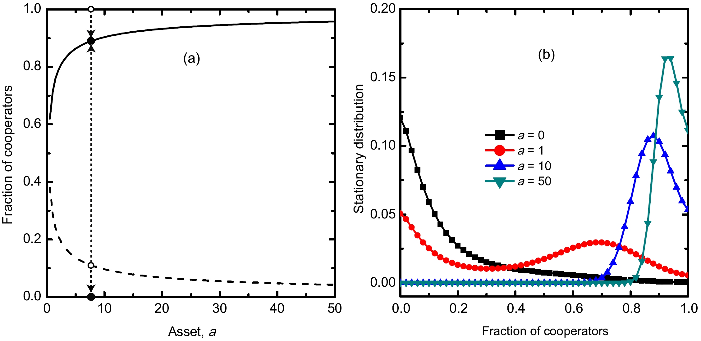
Figure 1: (Color online) Evolutionary dynamics of cooperation and defection in the collective-risk social dilemma with risky assets, as observed in well-mixed populations. (a) The stable equilibria (solid line) and unstable equilibria (dash line) as a function of the asset $a$ in infinite populations. (b) Stationary distribution of cooperation in finite populations for different values of individual asset $a$ (see legend) in the presence of mutation $\mu$ (see Appendix for details). Other parameters values are: $N=5$, $T=3$, $c/b=0.1$, $r=0.2$ in (a), and $N=5$, $T=3$, $Z=50$, $c/b=0.1$, $r=0.2$, $\mu=0.01$ in (b).

We here extend the collective-risk social dilemma game with risky assets to be played on the square lattice with periodic boundary conditions, where $L^{2}$ players are arranged into overlapping groups of size $N=5$ such that everyone is connected to its four nearest neighbors. Accordingly, each individual belongs to five different groups and it participates in five collective-risk games. Concerned for the loss of its assets, each individual $y$ aims to transfer these assets into those groups that have a lower probability to fail to reach the collective target. With the information at hand from the previous round of the game, player $y$ at time $t$ transfers the asset $a_{y}^{m}(t)$ into the group $G_{m}$ centered on player $m$ according to

$$a_{y}^{m}(t)=a\frac{[1-r_{m}(t-1)]^{\alpha}}{\sum_{n\in G_{y}}[1-r_{n}(t-1)]^{\alpha}},$$ (2)

where $r_{m}(t-1)=r$ if at time $t-1$ the number of cooperators $n_{c}^{m}(t-1)<T$ and $r_{m}(t-1)=0$ otherwise, and $\alpha$ is the allocation strength of the asset. Here, we mainly consider $\alpha\geq 0$, given that players generally prefer to allocate their asset into a relatively safe environment. We note that $\alpha=0$ means allocating the asset equally into all the groups without taking into account the information about risk. Accordingly, we will refer to this allocation scheme as uniform or equal. Conversely, $\alpha=+\infty$ means that individuals allocate their assets only into the most successful groups. We will refer to this as the fully rational allocation scheme. Lastly, for $0<\alpha<+\infty$, we have the so-called bounded rational allocation of assets.

In agreement with the above definitions, the payoff of player $y$ at time $t$ with strategy $S_{y}(t)$ and being member of the group that is centered on player $m$ is

$$P_{y}^{m}(t) = b\theta[n_{c}^{m}(t)-T]+b(1-r)\{1-\theta[n_{c}^{m}(t)-T]\}$$ (3)

$$- ra_{y}^{m}(t)\{1-\theta[n_{c}^{m}(t)-T]\}-cS_{y}(t).$$

The total payoff at time $t$ is then simply the accumulation of payoffs from each of the five individual groups where player $y$ is member, given as $P_{y}=\sum_{m}P_{y}^{m}(t)$.

After the accumulation of payoffs as described above, each player $y$ is allowed to learn from one randomly chosen neighbor $z$ with a probability given by the Fermi function Szabó and Tőke (1998); Szabó and Fáth (2007)

$$p=[1+\exp^{-\beta(P_{z}-P_{y})}]^{-1},$$ (4)

where in agreement with the settings in finite well-mixed populations (see Appendix for details), we use the intensity of selection $\beta=2.0$. Further with regards to the simulations details, we note that initially each player is designated either as a cooperator or defector with equal probability, and it equally allocates its asset into all the groups in which it is involved. Monte Carlo simulations are carried out for the population on the square lattice. We emphasize there exist ample evidence, especially for games that are governed by group interactions Szolnoki et al. (2009); Szolnoki and Perc (2011); Tanimoto (2013), in favor of the fact that using the square lattice suffices to reveal all the relevant evolutionary outcomes. Because the system may reach a stationary state where cooperators and defectors coexist in the finite structured population in the absence of mutation Nowak and May (1992), we determine the fraction of cooperators when it becomes time-independent. The final results were obtained over $100$ independent initial conditions to further increase accuracy, and their robustness has been tested on populations ranging from $L^{2}=2500$ to $10^{5}$ in size.

III Results

III.1 Well-mixed populations

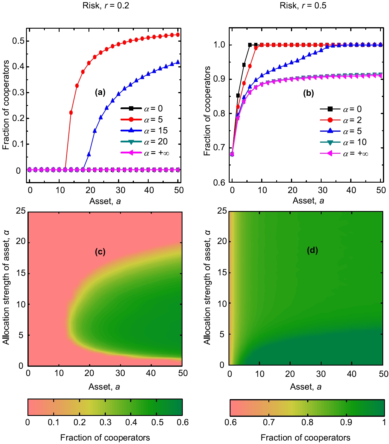
Figure 2: (Color online) Evolutionary dynamics of cooperation and defection in the collective-risk social dilemma with risky assets in structured populations. Top row depicts the stationary fraction of cooperators as a function of the asset $a$ for different values of allocation strength $\alpha$. The risk value is $r=0.2$ in (a) and $r=0.5$ in (b). Bottom row depicts the contour plot of the fraction of cooperators as a function of the asset $a$ and the allocation strength $\alpha$, as obtained for the risk value $r=0.2$ in (c) and $r=0.5$ in (d). Other parameters values are: $c/b=0.1$, $N=5$, and $T=3$.

We begin by showing the results obtained in well-mixed populations, when individual risky assets are incorporated into the collective-risk social dilemma as described by the minimal model. In infinite well-mixed populations, according to the replicator equation, it can be observed that only the presence of a high risk leads to two additional, interior equilibria beside the two boundary equilibria $x=0$ (stable) and $x=1$ (unstable) in the standard collective-risk social dilemma (Appendix A) Santos and Pacheco (2011). The unstable interior equilibrium, if it exists, divides the range $[0,1]$ of $x$ into two basins of attraction. In other words, when there is no risk or a low risk, the population has no interior equilibria, and the only stable equilibrium is at $x=0$, corresponding to the emergence of full defection [Fig. 1(a)]. However, in this unfavorable situation, we find that the introduction of risky assets can lead to the emergence of two mixed internal equilibria, which renders cooperation viable and in fact yields similar effects as a high risk environment. Furthermore, we find that as the asset increases, the stable interior equilibrium rapidly increases closely to one, while the unstable interior equilibrium rapidly decreases closely to zero [Fig. 1(a)] (see Appendix A for more analytical results).

In finite well-mixed population, we present the stationary distribution of cooperation for different values of asset $a$ for a population of size $Z=50$, where the group size $N=5$ and the threshold $T=3$ have been used, as shown in Fig. 1(b). It is worth pointing out that the stationary distribution characterizes the pervasiveness in time of a given configuration of the population in the presence of behavioral mutations (see Appendix for details). We see that in the absence of individual assets, the population spends most of the time in configurations where defectors prevail, especially at low risks of collective failure. However, when risky assets are introduced, the population begins to spend more time in configurations where cooperative behavior thrives. In particular, as the asset increases to a high value, the population spends most of the time in configurations where cooperators prevail, while it spends little time in configurations where defectors prevail.

These results highlight that the introduction of risky assets into the theoretical model of the collective-risk social dilemma Santos and Pacheco (2011) is found to raise the chances of coordinating actions and escaping the tragedy of the commons. Accordingly, we conclude that individual assets significantly enhance the positive impact of risk on the evolution of cooperation.

III.2 Structured populations

Figure 3: (Color online) Successful evolution of cooperation and the optimal allocation scheme of individual assets. Panel (a) depicts the stationary fraction of cooperators in dependence on the risk $r$ and the allocation strength $\alpha$, as obtained for $a=25$. Panel (b) depicts the typical dependence of the fraction of cooperators on the allocation strength $\alpha$ at $r=0.3$ and $r=0.5$, which are indicated by white dash lines in panel (a). Panel (c) depicts the optimal allocation strength $\alpha_{opt}$ that maximizes the fraction of cooperators in dependence on the risk $r$. Other parameters values are: $a=25$, $c/b=0.1$, $N=5$, and $T=3$.

We continue with presenting the results obtained in structured populations, where at each time step an individual participates in five collective-risk dilemma games and allocates its assets as described by the extended model. Figure 2 shows the fraction of cooperation in the stationary state for two different values of the risk $r$. It can be observed that the fraction of cooperators increases steadily with increasing the value of asset $a$, which is in agreement with the results obtained in well-mixed populations. Moreover, the fraction of cooperators increases with increasing $a$ irrespective of the value of risk $r$ and the allocation strength $\alpha$. More precisely, when the risk is small [Fig. 2(a) and (c)], defectors always dominate if $a<12$, and this regardless of the value of $\alpha$. On the other hand, if $a>12$, with increasing $\alpha$ the fraction of cooperators first increases, reaches a maximum, but then decreases slowly. This indicates that there exists an optimal allocation strength which can maximize the level of cooperation. In other words, neither uniform allocation nor completely rational allocation is optimal if the risk $r$ is small. Instead, only bounded rational allocation ensures the highest cooperation levels. When the risk is large [Fig. 2(b) and (d)] the fraction of cooperators still increases with increasing the asset value $a$, but decreases with increasing the allocation strength $\alpha$. Specifically, for $0<a<8$ the fraction of cooperators monotonously decreases with increasing $\alpha$. For larger assets, however, full cooperation is achieved by uniform allocation, but the same can also be attained with $\alpha$ values that are somewhat larger than zero. But as the value of $\alpha$ increases further, the fraction of cooperators slowly decreases. This can be counteracted by increasing the value of $a$, since then the range of $\alpha$ values where full cooperation is attained increases. Taken together, these results indicate that completely rational allocation of assets is not optimal for the successful evolution of cooperation. Instead, in low-risk situations bounded rational allocation of assets works best, while in high-risk situations the simplest uniform distribution of assets among all the groups is optimal.

In order to study how the reported dependence of the fraction of cooperators on allocation strength relies on the value of risk, we first show the stationary fraction of cooperators as a function of risk and allocation strength together at a certain asset value $a=25$ in Fig. 3(a). It can be observed that for risk $r<0.18$ defectors always dominate the population, regardless of the value of $\alpha$. For $0.18<r<0.46$, there exists an intermediate value of $\alpha$ that maximizes the fraction of cooperators. For $0.46<r<0.55$, the fraction of cooperators decreases with increasing $\alpha$. Finally, for even larger $r$ values, cooperators always dominate the population. Results presented in fig. 3(b) show two typical behaviors depicting the dependence of the cooperation level on the allocation strength at intermediate values of the risk, as reported in Fig. 2. We stress that the range of the risk values for the typical outcomes depends on other parameters, but the existence of these results is robust against the variations of the parameters (see Fig. 5 for details). Moreover, we compute the optimal value of the allocation strength $\alpha_{opt}$ for several intermediate risk values, as shown in Fig. 3(c). We see that $\alpha_{opt}$ decreases with increasing $r$, and finally reaches zero. This result highlights that with increasing the risk the optimal allocation scheme of risky assets gradually translates from bounded rational to the completely uniform allocation.

To explain these results, we continue by showing a series of snapshots depicting the spatial distribution of strategies over time. When producing the snapshots we use different colors not just for cooperators and defectors, but also for distinguishing whether an individuals’ central group is successful or not. More precisely, blue (yellow) color denotes cooperators (defectors) whose central group succeeds to reach the collective target. On the other hand, green (pink) color denotes cooperators (defectors) whose central group fails to reach the collective target.

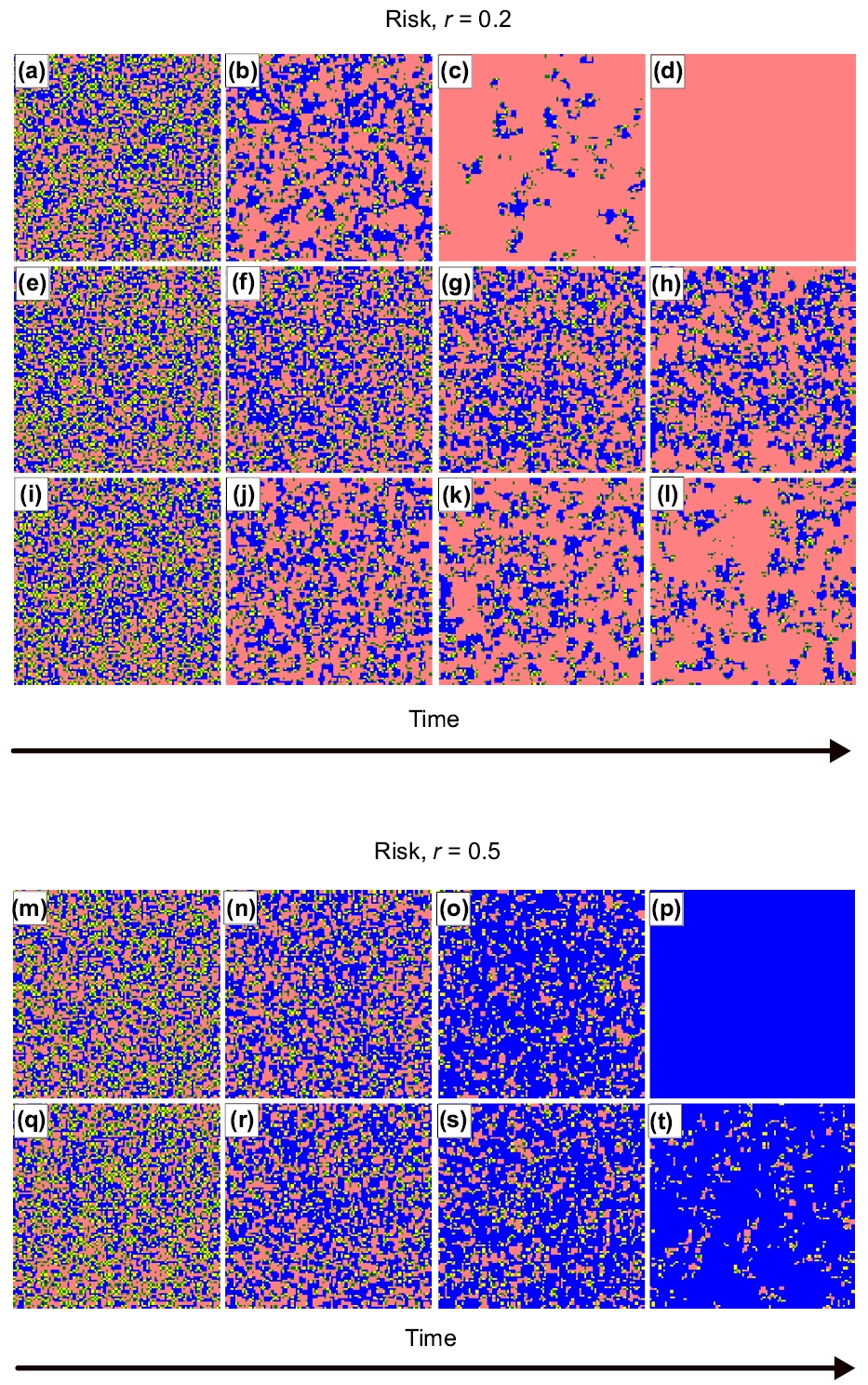
Figure 4: (Color online) Spatial pattern distribution as observed from an randomly initial state at risk $r=0.2$ (top three rows) and $r=0.5$ (bottom two rows). For $r=0.2$ the allocation strength is $\alpha=0$ [from (a) to (d)], $\alpha=5$ [from (e) to (h)], and $\alpha=15$ [from (i) to (l)]. For $r=0.5$ the allocation strength is $\alpha=0$ [from (m) to (p)] and $\alpha=10$ [from (q) to (t)]. Cooperators whose focal group succeeds (fails) are denoted blue (green), while defectors whose focal group succeeds (fails) are denoted yellow (pink). Other parameters are $T=3$, $c/b=0.1$, and $a=25$.

Figure 5: (Color online) The robustness of the evolution of cooperation in the collective-risk social dilemma with risky assets. Panel (a) depicts the fraction of cooperators as a function of the allocation strength $\alpha$ for different values of $T$ and $r$, as obtained for $a=25$, $N=5$, and $c/b=0.1$. Panel (b) depicts the fraction of cooperators as a function of the allocation strength $\alpha$ for different values of $r$ and $a$, as obtained for $T=3$, $N=5$ and a larger $c/b=0.2$ value. Panel (c) depicts the fraction of cooperators as a function of the allocation strength $\alpha$ for different values of $r$ and $a$, as obtained on a square lattice with Moore neighborhood (that is, the group size is $N=9$) for $a=25$, $c/b=0.1$, and $T=5$.

In the top three rows of Fig. 4, we show the representative sequences for three different values of $\alpha$, all obtained at a relatively low value of risk. When the risk is small, defectors have an evolutionary advantage over cooperators Santos and Pacheco (2011), and they utilize this advantage by gathering the benefit and ultimately becoming a successful strategy. For low $\alpha$ (top row of Fig. 4), both cooperators and defectors allocate the asset equally to all the groups. The uniform allocation cannot reverse the direction of invasion of defectors since both cooperators and defectors may lose a similar amount of asset at a low risk probability if they put the asset into a predominantly defective group. Gradually, the success of defectors easily drives the community into the tragedy of the commons, which is indicated by the emergence of pink defectors. Note that isolated islands of cooperators are in the sea of pink defectors, and finally they disappear completely. For intermediate values of $\alpha$ (second row of Fig. 4), individuals tends to put most of their asset into the successful groups. Thus, islands of cooperators can more easily preserve their assets than islands of defectors, even if the risk is low. Hence, cooperators do not lose their assets as much as defectors. Due to the introduction of risky assets, individual net payoffs, especially the payoffs from a failed group, depends strongly on the risk of collective failure. Thus, grouped blue cooperators are likely to have a higher payoff, at least locally. At the same time, yellow defectors remain successful if they are in the vicinity of cooperators, because then they can also preserve most of their assets and also enjoy most of the benefits from the surrounding successful groups. But once they invade their neighboring cooperators, they fast become pink defectors. Although pink defectors who are around blue cooperators also put most of their assets into the blue cooperators’ central group, and thus preserve the part of asset, they still put some assets into the neighboring unsuccessful groups where the centered individual is a green cooperator or a pink defector. Groups around green cooperators can partake the assets of pink defectors, which essentially protects the neighboring blue cooperators. Although the loss of assets happens with a low probability, it is still sufficiently probable for cooperators being able to resist the invasion of defectors and thus to form a mixed dynamical equilibrium in the stationary state. When $\alpha$ is further increased (third row of Fig. 4), defectors will lose a lower amount of their asset at the low risk probability since they put almost all their assets into the surrounding successful groups, if only such groups are present. The increment of $\alpha$ thus sustains the evolutionary advantage of defectors and the number of blue cooperators consequently decreases. A few isolated islands of cooperators can withstand the invasion of defectors because they locally get enough support from the grouped companions, but if $\alpha$ increases further (not shown), defectors raise to complete dominance.

The two bottom rows of Fig. 4 show representative snapshot sequences for two different values of $\alpha$, as obtained at a relatively high risk. For low values of $\alpha$ (fourth row of Fig. 4), blue cooperators do not lose their assets much and thus manage to have a higher net payoff then defectors. Hence, they can form compact clusters and expand across the whole population Chen et al. (2012a). On the contrary, pink defectors have more neighbors who are either also pink defectors or green cooperators. Thus, they lose some of their assets by placing them in the unsuccessful groups when $\alpha$ is zero or somewhat larger than zero. Even if $\alpha$ is increased, blue cooperators still lose less of their asset than other individuals, and can thus still have the highest net payoff. Therefore they have an evolutionary advantage, and can eventually dominate the whole population. When $\alpha$ is sufficiently large (bottom row of Fig. 4), both cooperators and defectors tend to allocate their assets predominantly into the successful surrounding groups. But grouped defectors still lose some of their assets because they simply do not have enough neighboring cooperators that would sustain successful groups. Hence, blue cooperators can still expand across the whole population, although some tiny specks of defectors manage to survive by holding on to the blue cooperators. As a result, a few defectors survive in the sea of cooperators.

To conclude, we report on the robustness of our findings by investigating changes in dependence on the cost-to-benefit ratio $c/b$, the collective target $T$, and the interaction structure, as shown in Fig. 5. When the threshold value changes, as shown in Fig. 5(a), we find that there exists an intermediate value of the allocation strength $\alpha$ that maximizes the fraction of cooperators at relatively small values of $r$, while the fraction of cooperators decreases with increasing allocation strengths for relatively large values of $r$. Although the range of $r$ values for the observation of the two typical behaviors varies as the threshold changes, as indicated by the results presented in Fig. 5(a), our main conclusion remain unchanged. Moreover, in Fig. 5(b), we find that our results are robust also against the variations of cost-to-benefit ratio $c/b$. In particular, as the $c/b$ ratio increases, the evolution of cooperation is impaired, which is in agreement with previous research Santos and Pacheco (2011); Chen et al. (2012a). But as we increase the value of the individual assets this trend is again reversed and cooperative behavior is as pervasive as by low $c/b$ ratios. Lastly, in Fig. 5(c), we change the interaction structure by replacing the Von Neumann neighborhood with the Moore neighborhood. It can be observed that there still exists an intermediate $\alpha$ value that maximizes the fraction of cooperators at relatively small values of $r$, and that the fraction of cooperators decrease with increasing $\alpha$ values at relatively large $r$ values. This indicates that our main conclusions are robust also against the changes in the structure of the interaction network.

IV Discussion

We have introduced and studied collective-risk social dilemma games with risky assets, and we have demonstrated how this can lead to elevated levels of cooperation in well-mixed and structured populations. The introduction of risky assets increases the stakes for each individual player, since insufficient contributions to the common pool result not only in the loss of personal endowments, but also in the loss of the assets. Thus, players are more prone to cooperating, and this regardless of their interaction range in the population. More precisely, we have shown that in infinite well-mixed populations new stable and unstable mixed steady states emerge, whereby the stable mixed steady state converges to full cooperation as either the risk of collective failure or the amount of risky assets increases. In finite well-mixed populations, we have shown that the introduction of risky assets drives the population towards configurations where cooperative behavior abounds. For comparison, in the absence of risky assets, finite well-mixed populations are prone to spend the majority of time in configurations where defectors prevail. In structured populations, where players have a limited interaction range, we have studied an extended collective-risk social dilemma games with risky assets, where the distribution of assets could be tuned by means of an allocation strength parameter. Among fully rational, bounded rational and uniform allocation, we have identified the latter as being optimal for the evolution of cooperation in high-risk situations. Conversely, in low-risk situations bounded rational allocation of assets works best. Most surprisingly, the fully rational allocation of assets only to the most successful groups, where in principle the assets would be least prone to being lost, is never optimal. We have explained these results with characteristic snapshot sequences of strategy distributions in the population, and we have identified pattern formation as being crucial for the observed evolutionary outcomes. We have also tested the robustness of our results with regards to variations of the cost-to-benefit ratio, the collective target to be reached with the contributions of players, and with regards to the variation of the interaction structure, always observing that at least qualitatively our main conclusions do not change and are fully robust.

As we have emphasized in the Introduction, the consideration of risky assets in the realm of the collective-risk social dilemma game is well aligned with reality, in which it is relatively straightforward to come up with examples where our model could apply. Our research shows that, at least in theory, such risky or unsecured, i.e., not immune to loss if the collective target is not reached, assets significantly promote cooperation and thus contribute to solving the collective-risk social dilemma. Research based on behavioral experiments has already considered individual assets Milinski et al. (2011), although the focus was on the interaction between wealth heterogeneity and intermediate climate targets. The experimental results show that, if players collectively face intermediate climate targets, then rich players are willing to substitute for missing contributions by poor players Milinski et al. (2011). Following this experimental study, a theoretical work by Abou Chakra and Traulsen Chakra and Traulsen (2014) further showed that rich players contribute on behalf of poor players only when their own external assets are worth protecting, and moreover, that rich players maintain cooperation by assisting poor players under a certain degree of uncertainty. Although the motivation behind our work and the setup are different, we hope that, collectively, the demonstrated importance of individual assets will inspire more research along this line, perhaps in the realm of other evolutionary games or in coevolutionary settings.

Appendix A: Evolutionary dynamics in infinite well-mixed populations

For studying the evolutionary dynamics in infinite well-mixed populations, we use the replicator equation Hofbauer and Sigmund (1998). To begin, we assume a large population, a fraction $x$ of which is composed of cooperators, the remaining fraction $(1-x)$ being defectors. Accordingly, the replicator equation is

$$\dot{x}=x(1-x)(P_{C}-P_{D}),$$ (5)

where $P_{C}$ and $P_{D}$ are the average payoffs of cooperators and defectors, respectively. Next, let groups of $N$ individuals be sampled randomly from the population. The average payoff of cooperators is

$$P_{C}=\sum_{j=0}^{N-1}\left(\begin{array}[]{c}N-1\\ j\end{array}\right)x^{j}(1-x)^{N-1-j}P_{C}(j+1),$$ (6)

while the average payoff of defectors is

$$P_{D}=\\ \sum_{j=0}^{N-1}\left(\begin{array}[]{c}N-1\\ j\end{array}\right)x^{j}(1-x)^{N-1-j}P_{D}(j).$$ (7)

With these definitions, the replicator equation has two boundary equilibria, namely $x=0$ and $x=1$, whereby full defection is stable while full cooperation is not. Interior equilibria, on the other hand, can be determined by equating $P_{C}$ and $P_{D}$, thus obtaining

$$P_{C}-P_{D}=\left(\begin{array}[]{c}N-1\\ T-1\end{array}\right)x^{T-1}(1-x)^{N-T}(b+a)r-c=0.$$ (8)

Furthermore, to determine the interior equilibria, we study the slope and the curvature of the function $G(x)$, which we define as

$$G(x)=\left(\begin{array}[]{c}N-1\\ T-1\end{array}\right)x^{T-1}(1-x)^{N-T}.$$ (9)

Note that $P_{C}-P_{D}=0$ is equivalent to $G(x)=c/[r(a+b)]$. We thus compute

$$G^{\prime}(x)=-\left(\begin{array}[]{c}N-1\\ T-1\end{array}\right)x^{T-2}(1-x)^{N-T-1}[1+(N-1)x-T],$$ (10)

from where it follows that, since $N>2$, $G^{\prime}(x)$ has a unique internal root at $\hat{x}=(T-1)/(N-1)$ when $1<T<N$. Moreover, $G^{\prime}(x)>0$ for $x<\hat{x}$ and $G^{\prime}(x)<0$ for $x>\hat{x}$. Accordingly, $G(\hat{x})$ is a unique interior maximum of $G(x)$.

Solving the equation $G(x)=c/[r(a+b)]$ thus yields the following conclusions:

1. When $G(\hat{x})>c/[r(a+b)]$, Eq. (5) has two interior equilibria, denoted by $x_{1}^{*}$ and $x_{2}^{*}$ with $x_{1}^{*}<\hat{x}<x_{2}^{*}$. Since $G^{\prime}(x)>0$ for $x<\hat{x}$ and $G^{\prime}(x)<0$ for $x>\hat{x}$, $x_{1}^{*}$ is an unstable equilibrium and $x_{2}^{*}$ is a stable equilibrium.

2. When $G(\hat{x})=c/[r(a+b)]$, Eq. (5) has only one interior equilibrium $\hat{x}$, which is a tangent point, and is thus unstable.

3. When $G(\hat{x})<c/[r(a+b)]$, Eq. (5) has no interior equilibria.

When $T=1$ or $T=N$, however, for $c/[r(a+b)]\geq 1$ Eq. (5) has no interior equilibria. While for $c/[r(a+b)]<1$, Eq. (5) has only one interior equilibrium $x^{*}$. Note that $x^{*}=1-\{c/[r(a+b)]\}^{1/(N-1)}$ is stable for $T=1$ since $G^{\prime}(x^{*})<0$, while $x^{*}=\{c/[r(a+b)]\}^{1/(N-1)}$ is unstable for $T=N$ since $G^{\prime}(x^{*})>0$.

Appendix B: Evolutionary dynamics in finite well-mixed populations

For studying the evolutionary dynamics in finite well-mixed populations, we consider a population of finite size $Z$. Here the average payoffs of cooperators and defectors in the population with $k$ cooperators are respectively given by

$$f_{C}(k) = \left(\begin{array}[]{c}Z-1\\ N-1\end{array}\right)^{-1}\sum_{j=0}^{N-1}\left(\begin{array}[]{c}k-1\\ j\end{array}\right)\left(\begin{array}[]{c}Z-k\\ N-j-1\end{array}\right)$$ (17)

$$\cdot P_{C}(j+1),$$ (18)

and

$$f_{D}(k) = \left(\begin{array}[]{c}Z-1\\ N-1\end{array}\right)^{-1}\sum_{j=0}^{N-1}\left(\begin{array}[]{c}k\\ j\end{array}\right)\left(\begin{array}[]{c}Z-k-1\\ N-j-1\end{array}\right)$$ (25)

$$\cdot P_{D}(j).$$ (26)

Next, we adopt the pair-wise comparison rule to study the evolutionary dynamics, based on which we assume that player $y$ adopts the strategy of player $z$ with a probability given by the Fermi function

$$p=[1+e^{-\beta(P_{z}-P_{y})}]^{-1},$$ (27)

where $\beta$ is the intensity of selection that determines the level of uncertainty in the strategy adoption process Szabó and Tőke (1998); Szabó and Fáth (2007). Without loosing generality, we use $\beta=2.0$ throughout this work.

With these definitions, the probability that the number of cooperators in the population increases or decreases by one is

$$T^{\pm}(k)=\frac{k}{Z}\frac{Z-k}{Z}[1+e^{\mp\beta[f_{C}(k)-f_{D}(k)]}]^{-1}.$$ (28)

Following previous research Santos and Pacheco (2011), we further introduce the mutation-selection process into the update rule, and compute the stationary distribution as the key quantity that determines the evolutionary dynamics in finite well-mixed populations. We note that, in the presence of mutations, the population will never fixate in any of the two possible absorbing states. Thus, the transition matrix of the complete Markov chain is

$$M=[p_{u,v}]_{(Z+1)\times(Z+1)}^{T},$$ (29)

where $p_{u,v}=0$ if $|u-v|>1$, otherwise $p_{u,u+1}=(1-\mu)T^{+}(u)+\mu(Z-u)/Z$, $p_{u,u-1}=(1-\mu)T^{-}(u)+\mu u/Z$ and $p_{u,u}=1-p_{u,u+1}-p_{u,u-1}$. Accordingly, the stationary distribution of the population, that is the average fraction of the time the population spends in each of the $Z+1$ states, is given by the eigenvector of the eigenvalue $1$ of the transition matrix $M$ Karlin and Taylor (1975). In the Results Section, Fig. 1(b) is obtained by using $\mu=0.01$.