Online Clique Clustering

Abstract

Clique clustering is the problem of partitioning the vertices of a graph into disjoint clusters, where each cluster forms a clique in the graph, while optimizing some objective function. In online clustering, the input graph is given one vertex at a time, and any vertices that have previously been clustered together are not allowed to be separated. The goal is to maintain a clustering with an objective value close to the optimal solution. For the variant where we want to maximize the number of edges in the clusters, we propose an online strategy based on the doubling technique. It has an asymptotic competitive ratio at most $15.646$ and an absolute competitive ratio at most $22.641$. We also show that no deterministic strategy can have an asymptotic competitive ratio better than $6$. For the variant where we want to minimize the number of edges between clusters, we show that the deterministic competitive ratio of the problem is $n-\omega(1)$, where $n$ is the number of vertices in the graph.

1 Introduction

The correlation clustering problem and its different variants have been extensively studied over the past decades; see e.g. [1, 5, 11]. The instance of correlation clustering consists of a graph whose vertices represent some objects and edges represent their similarity. Several objective functions are used in the literature, e.g., maximizing the number of edges within the clusters plus the number of non-edges between clusters (maximizing agreements), or minimizing the number of non-edges inside the clusters plus the number of edges outside them (minimizing disagreements). Bansal et al. [1] show that both the minimization of disagreement edges and the maximization of agreement edges versions are NP-hard. However, from the point of view of approximation the two versions differ. In the case of maximizing agreements this problem actually admits a PTAS, whereas in the case of minimizing disagreements it is APX-hard. Several efficient constant factor approximation algorithms are proposed for minimizing disagreements [1, 5, 11] and maximizing agreements [5].

Some correlation clustering problems may impose additional restrictions on the structure or size of the clusters. We study the variant, called clique clustering, where the clusters are required to form disjoint cliques in the underlying graph $G=(V,E)$. Here, we can maximize the number of edges inside the clusters or minimize the number of edges outside the clusters. These measures give rise to the maximum and minimum clique clustering problems respectively. The computational complexity and approximability of these problems have attracted attention recently [12, 15, 18], and they have numerous applications within the areas of gene expression profiling and DNA clone classification [2, 14, 18, 19].

We focus on the online variant of clique clustering, where the input graph $G$ is not known in advance. (See [3] for more background on online problems.) The vertices of $G$ arrive one at a time. Let $v_{t}$ denote the vertex that arrives at time $t$, for $t=1,2,\ldots$. When $v_{t}$ arrives, its edges to all preceding vertices $v_{1},\ldots,v_{t-1}$ are revealed as well. In other words, after step $t$, the subgraph of $G$ induced by $v_{1},v_{2},\ldots,v_{t}$ is known, but no other information about $G$ is available. In fact, we assume that even the number $n$ of vertices is not known upfront, and it is revealed only when the process terminates after step $t=n$.

Our objective is to construct a procedure that incrementally constructs and outputs a clustering based on the information acquired so far. Specifically, when $v_{t}$ arrives at step $t$, the procedure first creates a singleton clique ${\left\{v_{t}\right\}}$. Then it is allowed to merge any number of cliques (possibly none) in its current partitioning into larger cliques. No other modifications of the clustering are allowed. The merge operation in this online setting is irreversible; once vertices are clustered together, they will remain so, and hence, a bad decision may have significant impact on the final solution. This online model was proposed by Charikar et al. [4].

We avoid using the word “algorithm” for our procedure, since it evokes connotations with computational limits in terms of complexity. In fact, we place no limits on the computational power of our procedure and, to emphasize this, we use the word strategy rather than algorithm. This approach allows us to focus specifically on the limits posed by the lack of complete information about the input. Similar settings have been studied in previous work on online computation, for example for online medians [8, 9, 16], minimum-latency tours [6], and several other online optimization problems [10], where strategies with unlimited computational power were studied.

Our results.

We investigate the online clique clustering problem and provide upper and lower bounds for the competitive ratios for its maximization and minimization versions, that we denote MaxCC and MinCC, respectively.

Section 3 is devoted to the study of MaxCC. We first observe that the competitive ratio of the natural greedy strategy is linear in $n$. We then give a constant competitive strategy for MaxCC with asymptotic competitive ratio at most $15.646$ and absolute competitive ratio at most $22.641$. The strategy is based on the doubling technique often used in online algorithms. We show that the doubling approach cannot give a competitive ratio smaller than $10.927$. We also give a general lower bound, proving that there is no online strategy for MaxCC with competitive ratio smaller than $6$. Both these lower bounds apply also to asymptotic ratios.

In Section 4 we study online strategies for MinCC. We prove that no online strategy can have a competitive ratio of $n-\omega(1)$. We then show that the competitive ratio of the greedy strategy is $n-2$, matching this lower bound.

2 Preliminaries

We begin with some notation and basic definitions of the MaxCC and MinCC clustering problems. They are defined on an input graph $G=(V,E)$, with vertex set $V$ and edge set $E$. We wish to find a partitioning of the vertices in $V$ into clusters so that each cluster induces a clique in $G$. In addition, we want to optimize some objective function associated with the clustering. In the MaxCC case, this objective is to maximize the total number of edges inside the clusters, whereas in the MinCC case, we want to minimize the number of edges outside the clusters.

We will use the online model, proposed by Charikar et al. [4], and Mathieu et al. [17] for the online correlation clustering problem. Vertices (with their edges to previous vertices) arrive one at a time and must be clustered as soon as they arrive. Throughout the paper we will implicitly assume that any graph $G$ has its vertices ordered $v_{1},\ldots,v_{n}$, according to the ordering in which they arrive on input. The only two operations allowed are: ${\mbox{\it singleton}}(v_{t})$, that creates a singleton cluster containing the single vertex $v_{t}$, and ${\mbox{\it merge}}(C,C^{\prime})$, which merges two existing clusters $C,C^{\prime}$ into one, under the assumption that the resulting cluster induces a clique in $G$. This means that once two vertices are clustered together, they cannot be later separated.

For MaxCC, we define the profit of a clustering ${\cal C}={\left\{C_{1},\ldots,C_{k}\right\}}$ on a given graph $G=(V,E)$ to be the total number of edges in these cliques, that is $\sum_{i=1}^{k}\binom{|C_{i}|}{2}={\textstyle\frac{1}{2}}\sum_{i=1}^{k}|C_{i}|(|C_{i}|-1)$. Similarly, for MinCC, we define the cost of ${\cal C}$ to be the total number of edges outside the cliques, that is $|E|-\sum_{i=1}^{k}\binom{|C_{i}|}{2}$. For a graph $G$, we denote the optimal profit or cost for MaxCC and MinCC, respectively, by $\mbox{\sf{profit}}_{\scriptstyle\sf OPT}(G)$ and $\mbox{\sf{cost}}_{\scriptstyle\sf OPT}(G)$.

It is common to measure the performance of an online strategy by its competitive ratio. This ratio is defined as the worst case ratio between the profit/cost of the online strategy and the profit/cost of an offline optimal strategy, one that knows the complete input sequence in advance. More formally, for an online strategy ${\cal S}$, we define $\mbox{\sf{profit}}_{{\cal S}}(G)$ to be the profit of ${\cal S}$ when the input graph is $G=(V,E)$ and, similarly, let $\mbox{\sf{cost}}_{{\cal S}}(G)\stackrel{{\scriptstyle\text{def}}}{{=}}|E|-\mbox{\sf{profit}}_{{\cal S}}(G)$ be the cost of ${\cal S}$ on $G$.

We say that an online strategy ${\cal S}$ is $R$-competitive for MaxCC, if there is a constant $\beta$ such that for any input graph $G$ we have

$$R\cdot\mbox{\sf{profit}}_{{\cal S}}(G)+\beta\geq\mbox{\sf{profit}}_{\scriptstyle\sf OPT}(G).$$ (1)

Similarly ${\cal S}$ is $R$-competitive for MinCC, if there is a constant $\beta$ such that for any input graph $G$ we have

$$\mbox{\sf{cost}}_{{\cal S}}(G)\leq R\cdot\mbox{\sf{cost}}_{\scriptstyle\sf OPT}(G)+\beta.$$ (2)

The reason for defining the competitive ratio differently for maximization and minimization problems is to have all ratios being at least $1$. The smallest $R$ for which a strategy ${\cal S}$ is $R$-competitive is called the (asymptotic) competitive ratio of ${\cal S}$. The smallest $R$ for which ${\cal S}$ is $R$-competitive with $\beta=0$ is called the absolute competitive ratio of ${\cal S}$. (If it so happens that these minimum values do not exist, in both cases the competitive ratio is actually defined by the corresponding infimum.)

Note that an online strategy does not know when the last vertex arrives and, as a consequence, in order to be $R$-competitive, it needs to ensure that the corresponding bound, (1) or (2), is valid after each step.

3 Online Maximum Clique Clustering

In this section we study online MaxCC, the clique clustering problem where the objective is to maximize the number of edges within the cliques. The main results here are upper and lower bounds for the competitive ratio. For the upper bound, we give a strategy that uses a doubling technique to achieve a competitive ratio of at most $15.646$. For the lower bound, we show that no online strategy has a competitive ratio smaller than $6$. Additional results include a competitive analysis of the greedy strategy and a lower bound for doubling based strategies.

3.1 The Greedy Strategy for Online MaxCC

Greedy, the greedy strategy for MaxCC, merges each input vertex with the largest current cluster that maintains the clique property. This maximizes the increase in profit at this step. If no such merging is possible the vertex remains in its singleton cluster. Greedy strategies are commonly used as heuristics for a variety of online problems and can be shown to behave well for certain of them; e.g. [17]. We show that the solution of Greedy can be far from optimal for MaxCC.

For $n=1,2,3$, Greedy always finds an optimal clustering; see Figure 1, where all cases are shown. Therefore throughout the rest of this section we will be assuming that $n\geq 4$.

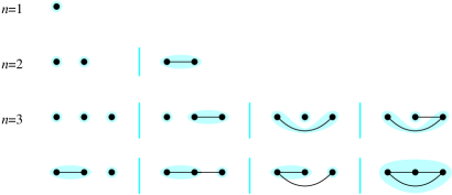
Figure 1: Greedy finds optimal clusterings (blue) for $n=1,2,3$. Vertices are released in order from left to right.

Theorem 1

Greedy has competitive ratio at least ${\lfloor n/2\rfloor}$ for MaxCC.

Proof: We first give the proof for the absolute ratio, and then extend it to the asymptotic ratio.

Consider an adversary that provides input to the strategy to make it behave as badly as possible. Our adversary creates an instance with $n$ vertices, numbered from $1$ to $n$. The odd vertices are connected to form a clique, and similarly the even vertices are connected to form a clique. In addition each vertex of the form $2i$, for $i=1,\ldots,{\lfloor(n-1)/2\rfloor}$, is connected to vertex $2i-1$; see Figure 2.

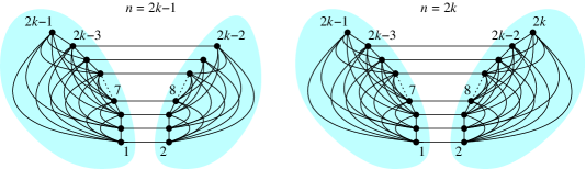
Figure 2: Illustrating the proof of Theorem 1 for odd and even $n$.

Greedy clusters the vertices as odd/even pairs, leaving the vertex $2k-1$ as a singleton, if $n=2k-1$ is odd and leaving both vertices $2k-1$ and $2k$ as singletons, if $n=2k$ is even. This generates a clustering of profit $\mbox{\sf{profit}}_{{\sf GDY}}(G)=k-1$. An optimal strategy clusters the odd vertices in one clique of size $k$ and the even vertices in another clique of size $k-1$ or $k$, depending on whether $n$ is odd or even. The profit for the optimal solution is $\mbox{\sf{profit}}_{{\scriptstyle\sf OPT}}(G)=(k-1)^{2}$, if $n$ is odd and $\mbox{\sf{profit}}_{{\scriptstyle\sf OPT}}(G)=k(k-1)$, if $n$ is even. Hence, the ratio between the optimum and the greedy solution is $k-1=(n-1)/2={\lfloor n/2\rfloor}$, if $n$ is odd, and $k=n/2={\lfloor n/2\rfloor}$, if $n$ is even; hence the worst case absolute competitive ratio of the greedy strategy is at least ${\lfloor n/2\rfloor}$.

To obtain the same lower bound on the asymptotic ratio, it suffices to notice that, if we follow the above adversary strategy, then for any $R<{\lfloor n/2\rfloor}$ and any constant $\beta>0$, we can find sufficiently large $n$ for which inequality (1) will be false. $\Box$

Next, we look at the upper bound for the greedy strategy.

Theorem 2

Greedy’s absolute competitive ratio for MaxCC is at most ${\lfloor n/2\rfloor}$.

Proof: As shown earlier, the theorem holds for $n=1,2,3$, so we can assume that $n\geq 4$. Fix an optimal clustering on $G$ that we denote ${\sf OPT}(G)$. Assume this clustering consists of $p$ non-singleton clusters of sizes $c_{1},\ldots,c_{p}$. The profit of ${\sf OPT}(G)$ is $\mbox{\sf{profit}}_{{\scriptstyle\sf OPT}}(G)={\textstyle\frac{1}{2}}\sum_{i=1}^{p}c_{i}(c_{i}-1)$. Let $k=\max_{i}c_{i}$ be the size of the maximum cluster of ${\sf OPT}(G)$.

Case 1: $k\leq{\lfloor n/2\rfloor}$. In this case, we can distribute the profit of each cluster of Greedy equally among the participating vertices; that is, if a vertex belongs to a Greedy cluster of size $c$, it will be assigned a profit of ${\textstyle\frac{1}{2}}(c-1)$. We refer to this quantity as charged profit. We now note that at most one vertex in each cluster of ${\sf OPT}(G)$ can be a singleton cluster in Greedy’s clustering, since otherwise Greedy would cluster any two such vertices together. This gives us that each vertex in a non-singleton cluster of ${\sf OPT}(G)$, except possibly for one, has charged profit at least ${\textstyle\frac{1}{2}}$. So the total profit charged to the vertices of an ${\sf OPT}(G)$ cluster of size $c_{i}$ is at least ${\textstyle\frac{1}{2}}(c_{i}-1)$. Therefore the profit ratio for this clique of ${\sf OPT}(G)$, namely the ratio between its optimal profit and Greedy’s charged profit, is at most

$$\frac{{\textstyle\frac{1}{2}}c_{i}(c_{i}-1)}{{\textstyle\frac{1}{2}}(c_{i}-1)}=c_{i}.$$

From this bound and the case assumption, all cliques of ${\sf OPT}(G)$ have profit ratio at most $k\leq{\lfloor n/2\rfloor}$, so the competitive ratio is also at most ${\lfloor n/2\rfloor}$.

Case 2: $k\geq{\lfloor n/2\rfloor}+1$. In this case there is a unique cluster $Q$ in ${\sf OPT}(G)$ of size $k$. The optimum profit is maximized if the graph has one other clique of size $n-k$, so

$$\mbox{\sf{profit}}_{{\scriptstyle\sf OPT}}(G)\;\leq\;{\textstyle\frac{1}{2}}k(k-1)+{\textstyle\frac{1}{2}}(n-k)(n-k-1)\;=\;{\textstyle\frac{1}{2}}(n^{2}+2k^{2}-2nk-n).$$ (3)

We now consider two sub-cases.

Case 2.1: Greedy’s profit is at least $k$. In this case, using (3) and $k\geq{\lfloor n/2\rfloor}+1\geq{\textstyle\frac{1}{2}}(n+1)$, the competitive ratio is at most

$$\frac{{\textstyle\frac{1}{2}}(n^{2}+2k^{2}-2nk-n)}{k}\;\leq\;{\textstyle\frac{1}{2}}(n-1)\;\leq\;{\lfloor n/2\rfloor}.$$

where the first inequality follows from simple calculus. (The function $(n^{2}+2k^{2}-2nk-n)-k(n-1)$ is non-positive for $k={\textstyle\frac{1}{2}}(n+1)$ and $k=n$ and its second derivative with respect to $k$ between these two values is positive.)

Case 2.2: Greedy’s profit is at most $k-1$. We show that in this case the profit of Greedy is in fact equal to $k-1$, and that Greedy’s clustering has a special form.

To prove this claim, consider those clusters of Greedy that intersect $Q$. For $i\geq 1$ and $j\geq 0$, let $d_{ij}$ be the number of these clusters that have $i$ vertices in $Q$ and $j$ outside $Q$. Note that at most one cluster of Greedy can be wholly contained in $Q$, as otherwise Greedy would merge such clusters if it had more. Denote by $\alpha$ the size of this cluster of Greedy contained in $Q$ (if it exists; if not, let $\alpha=0$). Let also $\beta=d_{11}$ and

$$\gamma\;=\;\sum_{\begin{subarray}{c}i,j\geq 1\\ i+j\geq 3\end{subarray}}\!\!id_{ij}\;=\;k-\alpha-\beta\;\geq\;0,$$

where $k=\sum_{i\geq 1,j\geq 0}id_{ij}$ counts the number of vertices in $Q$. The total profit of Greedy is at least

$${\textstyle\frac{1}{2}}\!\!\sum_{i\geq 1,j\geq 0}\!\!(i+j)(i+j-1)d_{ij}\; =\;{\textstyle\frac{1}{2}}\alpha(\alpha-1)+\beta+{\textstyle\frac{1}{2}}\!\!\sum_{\begin{subarray}{c}i,j\geq 1\\ i+j\geq 3\end{subarray}}\!\!(i+j)(i+j-1)d_{ij}$$

$$\geq\;{\textstyle\frac{1}{2}}\alpha(\alpha-1)+\beta+{\textstyle\frac{3}{2}}\!\!\sum_{\begin{subarray}{c}i,j\geq 1\\ i+j\geq 3\end{subarray}}\!\!id_{ij}$$

$$=\;{\textstyle\frac{1}{2}}\alpha(\alpha-1)+\beta+{\textstyle\frac{3}{2}}\gamma$$

$$=\;k+{\textstyle\frac{1}{2}}\alpha(\alpha-3)+{\textstyle\frac{1}{2}}\gamma\;\geq\;k-1+{\textstyle\frac{1}{2}}\gamma.$$

(The last inequality holds because, for integer values of $\alpha$, the expression $\alpha(\alpha-3)$ is minimized for $\alpha\in{\left\{1,2\right\}}$.) Combined with the case assumption that Greedy’s profit is at most $k-1$, we conclude that Greedy’s profit is indeed equal $k-1$ and, in addition, we have that $\gamma=0$ and $\alpha\in{\left\{1,2\right\}}$.

So, for $\alpha=1$, Greedy’s clustering consists of $k-1$ disjoint edges, each with exactly one endpoint in $Q$, plus a singleton vertex in $Q$. Thus $n\geq 2k-1$. As $k\geq{\lfloor n/2\rfloor}+1$, this is possible only when $n=2k-1$. By (3), the optimal profit in this case is at most $(k-1)^{2}$, so the ratio is at most $k-1={\lfloor n/2\rfloor}$.

For $\alpha=2$, Greedy’s clustering consists of $k-1$ edges, of which one is contained in $Q$ and the remaining ones have exactly one endpoint in $Q$. So $n\geq 2k-2$. If $n$ is odd, this and the bound $k\geq{\lfloor n/2\rfloor}+1$ would force $n=2k-1$, in which case the argument from the paragraph above applies. On the other hand, if $n$ is even, then these bounds will force $n=2k-2$. Then, by (3), the optimal profit is $k^{2}-3k+3$, so the competitive ratio is at most $(k^{2}-3k+3)/(k-1)=k-2+1/(k-1)\leq k-1={\lfloor n/2\rfloor}$, for $k\geq 2$. $\Box$

3.2 A Constant Competitive Strategy for MaxCC

In this section, we give our competitive online strategy ${\sf OCC}$. Roughly, the strategy works in phases. In each phase we consider the “batch” of nodes that have not yet been clustered with other nodes, compute an optimal clustering for this batch, and add these new clusters to the strategy’s clustering. The phases are defined so that the profit for consecutive phases increases exponentially.

The overall idea can be thought of as an application of the “doubling” strategy (see [10], for example), but in our case a subtle modification is required. Unlike other doubling approaches, in our strategy the phases are not completely independent: the clustering computed in each phase, in addition to the new nodes, needs to include the singleton nodes from earlier phases as well. This is needed, because in our objective function singleton clusters do not bring any profit.

We remark that one could alternatively consider using profit value $k^{2}/2$ for a clique of size $k$, which is a very close approximation to our function if $k$ is large. This would lead to a simpler strategy and much simpler analysis. However, this function is a bad approximation when the clustering involves many small cliques. This is, in fact, the most challenging scenario in the analysis of our algorithm, and instances with this property are also used in the lower bound proof.

3.2.1 The Strategy ${\sf OCC}$

Formally, our method works as follows. Fix some constant parameter $\gamma>1$. The strategy works in phases, starting with phase $j=0$. At any moment the clustering maintained by the strategy contains a set $U$ of singleton clusters. During phase $j$, each arriving vertex is added into $U$. As soon as there is a clustering of $U$ of profit at least $\gamma^{j}$, the strategy clusters $U$ according to this clustering and adds these new (non-singleton) clusters to its current clustering. (The vertices that form singleton clusters remain in $U$.) Then phase $j+1$ starts.

Note that phase $0$ ends as soon as one edge is revealed, since then it is possible for ${\sf OCC}$ to create a clustering with $\gamma^{0}=1$ edge. The last phase may not be complete; as a result all nodes released in this phase will be clustered as singletons. Observe also that the strategy never merges non-singleton cliques produced in different phases.

3.2.2 Asymptotic Analysis of ${\sf OCC}$

For the purpose of the analysis it is convenient to consider (without loss of generality) only infinite ordered graphs $G$, whose vertices arrive one at a time in some order $v_{1},v_{2},\ldots$, and we consider the ratios between the optimum profit and ${\sf OCC}$’s profit after each step. Furthermore, to make sure that all phases are well-defined, we will assume that the optimum profit for the whole graph $G$ is unbounded. Any finite instance can be converted into an infinite instance with this property by appending to it an infinite sequence of disjoint edges, without decreasing the worst-case profit ratio.

For a given instance (graph) $G$, define $\mbox{\sf{O}}_{j}(G)$ to be the total profit of the adversary at the end of phase $j$ in the ${\sf OCC}$’s computation on $G$. Similarly, $\mbox{\sf{S}}_{j}(G)$ denotes the total profit of Strategy OCC at the end of phase $j$ (including the incremental clustering produced in phase $j$). During phase $0$ the graph is empty, and at the end of phase $0$ it consists of only one edge, so $\mbox{\sf{S}}_{0}(G)=\mbox{\sf{O}}_{0}(G)=1$. For any phase $j>0$, the profit of ${\sf OCC}$ is equal to $\mbox{\sf{S}}_{j-1}(G)$ throughout the phase, except right after the very last step, when new non-singleton clusters are created. At the same time, the optimum profit can only increase. Thus the maximum ratio in phase $j$ is at most $\mbox{\sf{O}}_{j}(G)/\mbox{\sf{S}}_{j-1}(G)$. We can then conclude that, to estimate the competitive ratio of our strategy ${\sf OCC}$, it is sufficient to establish an asymptotic upper bound on numbers ${\sf R}_{j}$, for $j=1,2,\ldots$, defined by

$${\sf R}_{j}\;=\;\max_{G}\frac{\mbox{\sf{O}}_{j}(G)}{\mbox{\sf{S}}_{j-1}(G)},$$ (4)

where the maximum is taken over all infinite ordered graphs $G$. (While not immediately obvious, the maximum is well-defined. There are infinitely many prefixes of $G$ on which ${\sf OCC}$ will execute $j$ phases, due to the presence of singleton clusters. However, since these singletons induce an independent set after $j$ phases, only finitely many graphs $G$ need to be considered in this maximum.)

Our objective now is to derive a recurrence relation for the sequence ${\sf R}_{1},{\sf R}_{2},\ldots$. The value of ${\sf R}_{1}$ is some constant whose exact value is not important here since we are interested in the asymptotic ratio. (We will, however, estimate ${\sf R}_{1}$ later, when we bound the absolute competitive ratio in Section 3.2.3).

So now, assume that $j\geq 2$ and that ${\sf R}_{1},{\sf R}_{2},\ldots,{\sf R}_{j-1}$ are given. We want to bound ${\sf R}_{j}$ in terms of ${\sf R}_{1},{\sf R}_{2},\ldots,{\sf R}_{j-1}$. To this end, let $G$ be the graph for which ${\sf R}_{j}$ is realized, that is ${\sf R}_{j}=\mbox{\sf{O}}_{j}(G)/\mbox{\sf{S}}_{j-1}(G)$. With $G$ fixed, to avoid clutter, we will omit it in our notation, writing $\mbox{\sf{O}}_{j}=\mbox{\sf{O}}_{j}(G)$, $\mbox{\sf{S}}_{j}=\mbox{\sf{S}}_{j}(G)$, etc. In particular, ${\sf R}_{j}=\mbox{\sf{O}}_{j}/\mbox{\sf{S}}_{j-1}$.

We now claim that, without loss of generality, we can assume that in the computation on $G$, the incremental clusterings of Strategy OCC in each phase $1,2,\ldots,j-1$ do not contain any singleton clusters. (The clustering in phase $j$, however, is allowed to contain singletons.) We will refer to this property as the No-Singletons Assumption.

To prove this claim, we modify the ordering of $G$ as follows: if there is a phase $i<j$ such that the incremental clustering of $U$ in phase $i$ clusters some vertex $v$ from $U$ as a singleton, then delay the release of $v$ to the beginning of phase $i+1$. Postponing a release of a vertex that was clustered as a singleton in some phase $i<j$ to the beginning of phase $i+1$ does not affect the computation and profit of ${\sf OCC}$, because vertices from singleton clusters remain in $U$, and thus are available for clustering in phase $i+1$. In particular, the value of $\mbox{\sf{S}}_{j-1}$ will not change. This modification also does not change the value of $\mbox{\sf{O}}_{j}$, because the graph induced by the first $j$ phases is the same, only the ordering of the vertices has been changed. We can thus repeat this process until the No-Singletons Assumption is eventually satisfied. This proves the claim.

With the No-Singletons Assumption, the set $U$ is empty at the beginning of each phase $0,1,\ldots,j$. We can thus divide the vertices released in phases $0,1,\ldots,j$ into disjoint batches, where batch $B_{i}$ contains the vertices released in phase $i$, for $i=0,1,\ldots,j$. (At the end of phase $i$, right before the clustering is updated, we will have $B_{i}=U$.) For each such $i$, denote by $\Delta_{i}$ the maximum profit of a clustering of $B_{i}$. Then the total profit after $i$ phases is $\mbox{\sf{S}}_{i}=\Delta_{0}+\cdots+\Delta_{i}$, and, by the definition of ${\sf OCC}$, we have $\Delta_{i}\geq\gamma^{i}$ and $\mbox{\sf{S}}_{i}\geq(\gamma^{i+1}-1)/(\gamma-1)$.

For $i=0,1,\ldots,j$, let ${\bar{B}}_{i}=B_{0}\cup\ldots\cup B_{i}$ be the set of all vertices released in phases $0,\ldots,i$. Consider the optimal clustering of ${\bar{B}}_{j}$. In this clustering, every cluster has some number $a$ of nodes in ${\bar{B}}_{j-1}$ and some number $b$ of nodes in $B_{j}$. For any $a,b\geq 0$, let $k_{a,b}$ be the number of clusters of this form in the optimal clustering of ${\bar{B}}_{j}$. Then we have the following bounds, where the sums range over all integers $a,b\geq 0$.

$$\mbox{\sf{O}}_{j} =\sum{\binom{a+b}{2}}k_{a,b}$$ (5)

$$\mbox{\sf{O}}_{j-1} \geq\sum{\binom{a}{2}}k_{a,b}$$ (6)

$$\Delta_{j} \geq\sum{\binom{b}{2}}k_{a,b}$$ (7)

$$\mbox{\sf{S}}_{j-1} \geq{\textstyle\frac{1}{2}}\sum ak_{a,b}$$ (8)

Equality (5) is the definition of $\mbox{\sf{O}}_{j}$. Inequality (6) holds because the right hand side represents the profit of the optimal clustering of ${\bar{B}}_{j}$ restricted to ${\bar{B}}_{j-1}$, so it cannot exceed the optimal profit $\mbox{\sf{O}}_{j-1}$ for ${\bar{B}}_{j-1}$. Similarly, inequality (7) holds because the right hand side is the profit of the optimal clustering of ${\bar{B}}_{j}$ restricted to $B_{j}$, while $\Delta_{j}$ is the optimal profit of $B_{j}$. The last bound (8) follows from the fact that (as a consequence of the No-Singletons Assumption) our strategy does not have any singleton clusters in ${\bar{B}}_{j-1}$. This means that in OCC’s clustering of ${\bar{B}}_{j-1}$ (which has $\sum ak_{a,b}$ vertices) each vertex has an edge included in some cluster, so the number of these edges must be at least ${\textstyle\frac{1}{2}}\sum ak_{a,b}$.

We can also bound $\Delta_{j}$, the strategy’s profit increase, from above. We have $\Delta_{0}=1$ and for each phase $j\geq 1$,

$$\Delta_{j}\;\leq\;\gamma^{j}+{\textstyle\frac{1}{2}}(\sqrt{8\gamma^{j}+1}+1)\;<\;\gamma^{j}+\sqrt{2}\gamma^{j/2}+2-\sqrt{2}.$$ (9)

To show (9), suppose that phase $j$ ends at step $t$ (that is, right after $v_{t}$ is revealed). Consider the optimal partitioning ${\cal P}$ of $B_{j}$, and let the cluster $c$ containing $v_{t}$ in ${\cal P}$ have size $p+1$. If we remove $v_{t}$ from this partitioning, we obtain a partitioning ${\cal P}^{\prime}$ of the batch after step $t-1$, whose profit must be strictly smaller than $\gamma^{j}$. So the profit of ${\cal P}$ is smaller than $\gamma^{j}+p$. In partitioning ${\cal P}^{\prime}$, the cluster $c-\{v_{t}\}$ has size $p$. We thus obtain that $\binom{p}{2}<\gamma^{j}$, because, in the worst case, ${\cal P}$ consists only of the cluster $c$. This gives us $p<{\textstyle\frac{1}{2}}(\sqrt{8\gamma^{j}+1}+1)$. The second inequality in (9) follows by routine calculation.

From (9), by adding up all profits from phases $0,\ldots,j$, we obtain an upper bound on the total profit of the strategy,

$$\mbox{\sf{S}}_{j}<\frac{\gamma^{j+1}-1}{\gamma-1}+\sqrt{2}\cdot\frac{\gamma^{(j+1)/2}-\gamma^{1/2}}{\gamma^{1/2}-1}+(2-\sqrt{2})j+1.$$ (10)

Lemma 3.1

For any pair of non-negative integers $a$ and $b$, the inequality

$${\binom{a+b}{2}}\leq(x+1){\binom{a}{2}}+\frac{x+1}{x}{\binom{b}{2}}+a$$

holds for any $0<x\leq 1$.

Proof: Define the function

$$F(a,b,x) =2x(x+1){\binom{a}{2}}+2(x+1){\binom{b}{2}}+2ax-2x{\binom{a+b}{2}}$$

$$=a^{2}x^{2}-ax^{2}+2ax+b^{2}-b-2abx$$

$$=(b-ax)^{2}+ax(2-x)-b,$$

i.e., $2x$ times the difference between the right hand side and the left hand side of the inequality above. It is sufficient to show that $F(a,b,x)$ is non-negative for integers $a,b\geq 0$ and $0<x\leq 1$.

Consider first the cases when $a\in\{0,1\}$ or $b\in\{0,1\}$. $F(0,b,x)=b(b-1)\geq 0$, for any non-negative integer $b$ and any $x$. $F(a,0,x)=ax(ax-x+2)\geq ax(ax+1)>0$, for any positive integer $a$ and $0<x\leq 1$. $F(a,1,x)=x^{2}a(a-1)\geq 0$, for any positive integer $a$ and any $x$. $F(1,2,x)=2-2x\geq 0$, for $0<x\leq 1$, and $F(1,b,x)=b^{2}-b+2x-2bx\geq b^{2}-3b\geq 0$, for any integer $b\geq 3$ and $0<x\leq 1$.

Thus, it only remains to show that $F(a,b,x)$ is non-negative when both $a\geq 2$ and $b\geq 2$. The function $F(a,b,x)$ is quadratic in $x$ and hence has one local minimum at $x_{0}=\frac{b-1}{a-1}$, as can be easily verified by differentiating $F$ in $x$. Therefore, in the case when $a\leq b$, $F(a,b,x)\geq F(a,b,1)=(b-a)^{2}-(b-a)\geq 0$, for $0<x\leq 1$. In the case when $a>b$, we have that $F(a,b,x)\geq F(a,b,\frac{b-1}{a-1})=\frac{(a-b)(b-1)}{a-1}>0$, which completes the proof. $\Box$

Suppose that $j\geq 2$ and fix some parameter $x$, $0<x<1$, whose value we will determine later. Using Lemma 3.1, the bounds (5)–(8), and the definition of ${\sf R}_{j-1}$, we obtain

$${\sf R}_{j}\mbox{\sf{S}}_{j-1}=\mbox{\sf{O}}_{j} =\sum{\binom{a+b}{2}}k_{a,b}$$

$$\leq(x+1)\sum{\binom{a}{2}}k_{a,b}+\frac{x+1}{x}\sum{\binom{b}{2}}k_{a,b}+\sum ak_{a,b}$$

$$\leq(x+1)\mbox{\sf{O}}_{j-1}+\frac{x+1}{x}\Delta_{j}+2\mbox{\sf{S}}_{j-1}$$ (11)

$$\leq(x+1){\sf R}_{j-1}\mbox{\sf{S}}_{j-2}+\frac{x+1}{x}\Delta_{j}+2\mbox{\sf{S}}_{j-1}.$$

Thus ${\sf R}_{j}$ satisfies the recurrence

$${\sf R}_{j}\leq\frac{x+1}{x\mbox{\sf{S}}_{j-1}}\left[\rule[0.0pt]{0.0pt}{12.91663pt}\,x\mbox{\sf{S}}_{j-2}{\sf R}_{j-1}+\Delta_{j}\,\right]+2.$$ (12)

From inequalities (9) and (10), we have

$$\Delta_{i}=\gamma^{i}(1+o(1))\quad\textrm{and}\quad\mbox{\sf{S}}_{i}=\frac{\gamma^{i+1}(1+o(1))}{\gamma-1}.$$

for all $i=0,1,\ldots,j$. Above, we use the notation $o(1)$ to denote any function that tends to $0$ as the phase index $i$ goes to infinity (with $x$ and $\gamma$ assumed to be some fixed constants, still to be determined). Substituting into recurrence (12), we get

$${\sf R}_{j}\leq\Big{(}\frac{x+1}{\gamma}+o(1)\Big{)}\cdot{\sf R}_{j-1}+\frac{(x+1)(\gamma-1)}{x}+2+o(1).$$ (13)

Now define

$${\sf R}=\frac{\gamma(\gamma x+x+\gamma-1)}{x(\gamma-x-1)}.$$ (14)

Lemma 3.2

Assume that $x+1<\gamma$, then ${\sf R}_{j}={\sf R}+o(1)$.

Proof: The proof is by routine calculus, so we only provide a sketch. For all $j\geq 1$ let $\rho_{j}={\sf R}_{j}-{\sf R}$. Then, substituting this into (13) and simplifying, we obtain that the $\rho_{j}$’s satisfy the recurrence

$$\rho_{j}\leq\Big{(}\frac{x+1}{\gamma}+o(1)\Big{)}\cdot\rho_{j-1}+o(1).$$ (15)

Since $x+1<\gamma$, this implies that $\rho_{j}=o(1)$, and the lemma follows. $\Box$

Lemma 3.2 gives us (essentially) a bound of ${\sf R}$ on the asymptotic competitive ratio of Strategy OCC, for fixed values of parameters $\gamma$ (of the strategy) and $x$ (of the analysis). We can now choose $\gamma$ and $x$ to make ${\sf R}$ as small as possible. ${\sf R}$ is minimized for parameters $x={\textstyle\frac{1}{2}}(5-\sqrt{13})\approx 0.697$ and $\gamma={\textstyle\frac{1}{2}}(3+\sqrt{13})\approx 3.303$, yielding

$${\sf R}={\textstyle\frac{1}{6}}(47+13\sqrt{13})\approx 15.646.$$

Using Lemma 3.2, for each graph $G$ and phase $j$, we have that $\mbox{\sf{O}}_{j}(G)\leq({\sf R}+o(1))\mbox{\sf{S}}_{j-1}(G)$. Since, in fact, ${\sf R}<15.646$, this implies that $\mbox{\sf{O}}_{j}(G)\leq 15.646\cdot\mbox{\sf{S}}_{j-1}(G)$, as long as $j$ is large enough. Thus $\mbox{\sf{O}}_{j}(G)\leq 15.646\cdot\mbox{\sf{S}}_{j-1}(G)+O(1)$ for all phases $j$. As we discussed earlier, bounding $\mbox{\sf{O}}_{j}(G)$ in terms of $\mbox{\sf{S}}_{j-1}(G)$ like this is sufficient to establish a bound on the (asymptotic) competitive ratio of Strategy ${\sf OCC}$. Summarizing, we obtain the following theorem.

Theorem 3

The asymptotic competitive ratio of Strategy ${\sf OCC}$ is at most $15.646$.

3.2.3 Absolute Competitive Ratio

In fact, for $\gamma={\textstyle\frac{1}{2}}(3+\sqrt{13})$, Strategy OCC has a low absolute competitive ratio as well. We show that this ratio is at most $22.641$. The argument uses the same value of parameter $x={\textstyle\frac{1}{2}}(5-\sqrt{13})$, but requires a more refined analysis.

When phase 0 ends, the competitive ratio is $1$. For $j\geq 1$, let $\mbox{\sf{O}}^{\prime}_{j}$ be the optimal profit right before phase $j$ ends. (Earlier we used $\mbox{\sf{O}}_{j}$ to estimate this value, but $\mbox{\sf{O}}_{j}$ also includes the profit for the last step of phase $j$.) It remains to show that for phases $j\geq 1$ we have ${\sf R}^{\prime}_{j}\leq 22.641$, where ${\sf R}^{\prime}_{j}=\mbox{\sf{O}}^{\prime}_{j}/\mbox{\sf{S}}_{j-1}$.

By exhaustively analyzing the behavior of Strategy ${\sf OCC}$ in phase 1, taking into account that $\gamma\approx 3.303>3$, we can establish that ${\sf R}^{\prime}_{1}=10$. We will then bound the remaining ratios using a refined version of recurrence (12).

We start by estimating ${\sf R}^{\prime}_{1}$. Let $t$ be the last step of phase 1. Since $\gamma\approx 3.303$, after step $t-1$ the profit of the vertices released in phase 1 is at most $3$. We can assume that phase 0 has only two vertices $v_{1},v_{2}$ connected by an edge. Let $H$ be the graph induced by $v_{1},\ldots,v_{t-1}$ and $H^{\prime}$ be its subgraph induced by $v_{3},\ldots,v_{t-1}$. We thus want to bound the optimal profit of $H$, under the assumption that the optimal profit of $H^{\prime}$ is at most $3$.

Denote by ${\bf K}_{i}$ the clique with $i$ vertices. The optimal clustering of $H^{\prime}$ cannot include a ${\bf K}_{4}$, and either

1. $H^{\prime}$ has no ${\bf K}_{3}$, and it has at most three ${\bf K}_{2}$ cliques, or

2. $H^{\prime}$ has a ${\bf K}_{3}$, with each edge of $H^{\prime}$ having at least one endpoint in this ${\bf K}_{3}$.

In Case 1, $H$ cannot contain a ${\bf K}_{5}$. If a clustering of $H$ includes a ${\bf K}_{4}$ then this ${\bf K}_{4}$ contains $v_{1}$, $v_{2}$, and two vertices from phase $1$. So in addition to this ${\bf K}_{4}$ it can at best include two ${\bf K}_{2}$’s, for a total profit of at most $8$. In Case 2, if a clustering of $H$ includes a ${\bf K}_{5}$, then it cannot include any cluster except this ${\bf K}_{5}$, so its profit is $10$. If a clustering of $H$ includes a ${\bf K}_{4}$, then this ${\bf K}_{4}$ must contain at least one of $v_{1}$ and $v_{2}$, and it may include at most one other clique of type ${\bf K}_{2}$. This will give a total profit of at most $7$. Summarizing, in each case the profit of $H$ is at most $10$ giving us ${\sf R}^{\prime}_{1}\leq 10$, as claimed.

For phases $j\geq 2$, we can tabulate upper bounds for ${\sf R}^{\prime}_{j}$ by explicitly computing the ratios ${\sf R}^{\prime}_{j}=\mbox{\sf{O}}^{\prime}_{j}/\mbox{\sf{S}}_{j-1}$ using the following modification of recurrence (12),

$${\sf R}^{\prime}_{j}\leq\frac{x+1}{x\mbox{\sf{S}}_{j-1}}\left[\rule[0.0pt]{0.0pt}{12.91663pt}\,x\mbox{\sf{S}}_{j-2}{\sf R}^{\prime}_{j-1}+\Delta_{j}\,\right]+2,$$ (16)

where we use the more exact bounds

$$\lceil\gamma^{j}\rceil\leq\Delta_{j}\leq{\lfloor\gamma^{j}+{\textstyle\frac{1}{2}}(\sqrt{8\gamma^{j}+1}+1)\rfloor},$$

obtained by rounding the bounds $\Delta_{j}\geq\gamma^{j}$ and (9), which we can do because $\Delta_{j}$ is integral. From the definition of $\mbox{\sf{S}}_{j}\stackrel{{\scriptstyle\text{def}}}{{=}}1+\sum_{i=1}^{j}\Delta_{i}$ we compute the first few estimates as shown in Table 1.

Table 1: Some initial bounds for $\mbox{\sf{S}}_{j}$ and the absolute competitive ratio.

Phase ($j$)	0	1	2	3	4	5	6	7	8
min $\mbox{\sf{S}}_{j}$	1	5	16	53	172	566	1 864	6 152	20 311
max $\mbox{\sf{S}}_{j}$	1	7	23	68	202	623	1 972	6 352	20 679
Bound (${\sf R}^{\prime}_{j}$)	1.000	10.000	13.185	18.636	21.881	22.641	21.516	19.925	18.509

To bound the sequence $\{{\sf R}^{\prime}_{j}\}_{j\geq 9}$ we rewrite recurrence (16) as

$${\sf R}^{\prime}_{j}\leq\frac{(x+1)\mbox{\sf{S}}_{j-2}}{\mbox{\sf{S}}_{j-1}}\cdot{\sf R}^{\prime}_{j-1}+\frac{(x+1)\Delta_{j}}{x\mbox{\sf{S}}_{j-1}}+2=\alpha_{j}{\sf R}^{\prime}_{j-1}+\beta_{j},$$

and bound $\alpha_{j}$ and $\beta_{j}$ using (9) and (10). With routine calculations, we can establish the bounds $\alpha_{j}<{\textstyle\frac{3}{5}}$ and $\beta_{j}<8$, for $j\geq 8$.

Thus, ${\sf R}^{\prime}_{j}\leq\hat{{\sf R}}_{j}$, where $\hat{{\sf R}}_{j}$ is

$$\hat{{\sf R}}_{j}={\textstyle\frac{3}{5}}\hat{{\sf R}}_{j-1}+8\leq 20-a\left({\textstyle\frac{3}{5}}\right)^{j},$$

for $j\geq 8$ and some positive constant $a$. The sequence $\{\hat{\sf R}_{j}\}_{j\geq 9}$, is thus bounded above by a monotonically growing function of $j$ having limit $20$ and hence $\hat{\sf R}_{j}\leq 20$ for every $j\geq 9$.

Combining this with the bounds estimated in Table 1, we see that the largest bound on ${\sf R}^{\prime}_{j}$ is $22.641$ given for $j=5$. We can thus conclude that the absolute competitive ratio of OCC is at most $22.641$.

We can improve on the absolute competitive ratio by choosing different values for $\gamma$ and $x$ that allow the asymptotic competitive ratio to increase slightly. The optimal values can be found empirically (using mathematical software) to be $\gamma=4.02323428$ and $x=0.823889$, giving asymptotic competitive ratio 15.902 and absolute competitive ratio 20.017.

3.3 A Lower Bound for Strategy ${\sf OCC}$

In this section we will show that, for any choice of $\gamma$, the worst-case ratio of Strategy ${\sf OCC}$ is at least $10.927$.

Denote by $B_{j}$ the $j$-th batch, that is the vertices released in phase $j$. We will use notation $\mbox{\sf{S}}_{j}$ for the profit of ${\sf OCC}$ and $\mbox{\sf{O}}_{j}$ for the optimal profit on the sub-instance consisting of the first $j$ batches. To avoid clutter we will omit lower order terms in our calculations. In particular, we focus on $j$ being large enough, treating $\gamma^{j}$ as integer, and all estimates for $\mbox{\sf{S}}_{j}$ and $\mbox{\sf{O}}_{j}$ given below are meant to hold within a factor of $1\pm o(1)$. (The asymptotic notation is with respect to the phase index $j$ tending to $\infty$.)

We start with a simpler construction that shows a lower bound of $9$; then we will explain how to improve it to $10.927$. In the instance we construct, all batches will be disjoint, with the $j$th batch $B_{j}$ having $2\gamma^{j}$ vertices connected by $\gamma^{j}$ disjoint edges (that is, a perfect matching). We will refer to these edges as batch edges. The edges between any two batches $B_{i}$ and $B_{j}$, for $i<j$, form a complete bipartite graph. These edges will be called cross edges; see Figure 3.

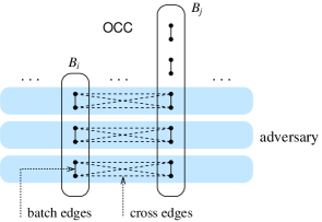
Figure 3: The lower bound example for Strategy ${\sf OCC}$. The figure shows two batches $B_{i}$ and $B_{j}$, for $i<j$. Batch edges, drawn with solid lines, are collected by Strategy ${\sf OCC}$. Dashed lines show cross edges that are in the adversary’s clustering. Shaded regions illustrate the cliques in the adversary’s clustering.

At the end of each phase $j$, the strategy will collect all $\gamma^{j}$ edges inside $B_{j}$. Therefore, by summing up the geometric sequence, right before the end of phase $j$ (before the strategy adds the new edges from $B_{j}$ to its clustering), the strategy’s profit is

$$\mbox{\sf{S}}_{j-1}=\sum_{i=0}^{j-1}\gamma^{i}\leq\frac{\gamma^{j}}{\gamma-1}.$$

After the first $j$ phases, the adversary’s clustering consists of cliques $C_{p}$, $p=0,1,\ldots,\gamma^{j}-1$, where $C_{p}$ contains the $p$-th edge (that is, its both endpoints) from each batch $B_{i}$ for $i=p,p+1,\ldots,j$; see Figure 3. We claim that the adversary gain after $j$ phases satisfies

$$\mbox{\sf{O}}_{j}\geq\mbox{\sf{O}}_{j-1}+\gamma^{j}+4\sum_{i=0}^{j-1}\gamma^{i}=\mbox{\sf{O}}_{j-1}+\frac{(\gamma+3)\gamma^{j}}{\gamma-1}.$$ (17)

(Recall that all equalities and inequalities in this section are assumed to hold only within a factor of $1\pm o(1)$.) We now justify this bound. The second term $\gamma^{j}$ is simply the number of batch edges in $B_{j}$. To see where each term $4\gamma^{i}$ comes from, consider the $p$-th batch edge from $B_{i}$, for $i<j$. When we add $B_{j}$ after phase $j$, the adversary can add the $4$ cross edges connecting this edge’s endpoints to the endpoints of the $p$th batch edge in $B_{j}$ to $C_{p}$. Overall, this will add $4\gamma^{i}$ cross edges between $B_{i}$ and $B_{j}$ to the existing adversary’s cliques.

From recurrence (17), by simple summation, we get

$$\mbox{\sf{O}}_{j}\geq\frac{(\gamma+3)\gamma^{j+1}}{(\gamma-1)^{2}}.$$

Dividing it by ${\sf OCC}$’s profit of at most $\gamma^{j}/(\gamma-1)$, we obtain that the ratio is at least $\frac{\gamma(\gamma+3)}{\gamma-1}$, which, by routine calculus, is at least $9$.

We now outline an argument showing how to improve this lower bound to $10.927$. The new construction is almost identical to the previous one, except that we change the very last batch $B_{j}$. As before, each batch $B_{i}$, for $i<j$, has $\gamma^{i}$ disjoint edges. Batch $B_{j}$ will also have $\gamma^{j}$ edges, but they will be grouped into $q={\textstyle\frac{1}{3}}\gamma^{j}$ disjoint triangles. (So $B_{j}$ has $\gamma^{j}$ vertices.) For $p=0,1,\ldots,q-1$, we add the $p$-th triangle to clique $C_{p}$. (If $q>\gamma^{j-1}$, the last $q-\gamma^{j-1}$ triangles will form new cliques.)

This modification will preserve the number of edges in $B_{j}$ and thus it will not affect the strategy’s profit. But now, for each $i=0,1,\ldots,j-1$ and each $p=0,1,\ldots,\min(q,\gamma^{i})-1$, we can connect the two vertices in $B_{i}\cap C_{p}$ to three vertices in $B_{j}$, instead of two. This creates two new cross edges that will be called extra edges. It should be intuitively clear that the number of these extra edges is $\Omega(\gamma^{j})$, which means that this new construction gives a ratio strictly larger than $9$.

Specifically, to estimate the ratio, we will distinguish three cases, depending on the value of $\gamma$. Suppose first that $\gamma\geq 3$. Then $q\geq\gamma^{j-1}$, so the number of extra edges is $2\sum_{i=0}^{j-1}\gamma^{i}=2\gamma^{j}/(\gamma-1)$, because each vertex in $B_{0}\cup B_{1}\cup\cdots\cup B_{j-1}$ is now connected to three vertices in $B_{j}$, not two. Thus the new optimal profit is

$$\mbox{\sf{O}}^{\prime}_{j}=\mbox{\sf{O}}_{j}+\frac{2\gamma^{j}}{\gamma-1}=\frac{(\gamma^{2}+5\gamma-2)\gamma^{j}}{(\gamma-1)^{2}}.$$

Dividing by ${\sf OCC}$’s profit, the ratio is at least $\frac{\gamma^{2}+5\gamma-2}{\gamma-1}$, which is at least $11$ for $\gamma\geq 3$.

The second case is when $\sqrt{3}\leq\gamma\leq 3$. Then $\gamma^{j-2}\leq q\leq\gamma^{j-1}$. In this case all vertices in $B_{0}\cup B_{1}\cup\cdots\cup B_{j-2}$ and ${\textstyle\frac{2}{3}}\gamma^{j}$ vertices in $B_{j-1}$ get an extra edge, so the number of extra edges is $2\gamma^{j-1}/(\gamma-1)+{\textstyle\frac{2}{3}}\gamma^{j}$. Therefore the new adversary profit is

$$\mbox{\sf{O}}^{\prime}_{j}=\mbox{\sf{O}}_{j}+2\,\frac{\gamma^{j-1}}{\gamma-1}+{\textstyle\frac{2}{3}}\gamma^{j}=\frac{(5\gamma^{3}+5\gamma^{2}+8\gamma-6)\gamma^{j-1}}{3(\gamma-1)^{2}}.$$

We thus have that the ratio is at least $\frac{5\gamma^{3}+5\gamma^{2}+8\gamma-6}{3\gamma(\gamma-1)}$. Minimizing this quantity, we obtain that the ratio is at least $10.927$.

The last case is when $1<\gamma\leq\sqrt{3}$. In this case, even using the earlier strategy (without any extra edges), we have that the ratio $\mbox{\sf{O}}_{j}/\mbox{\sf{S}}_{j-1}=\frac{\gamma(\gamma+3)}{\gamma-1}$ is at least $3+6\sqrt{3}\approx 11.2$ (it is minimized for $\gamma=\sqrt{3}$).

3.4 A Lower Bound of 6 for MaxCC

We now prove that any deterministic online strategy ${\cal S}$ for the clique clustering problem has competitive ratio at least $6$. We present the proof for the absolute competitive ratio and explain later how to extend it to the asymptotic ratio. The lower bound is established by showing, for any constant $R<6$, an adversary strategy for constructing an input graph $G$ on which $\mbox{\sf{profit}}_{{\scriptstyle\sf OPT}}(G)\geq R\cdot\mbox{\sf{profit}}_{{\cal S}}(G)$, that is the optimal profit is at least $R$ times the profit of ${\cal S}$.

Skeleton trees.

Fix some non-negative integer $D$. (Later we will make the value of $D$ depend on $R$.) It is convenient to describe the graph constructed by the adversary in terms of its underlying skeleton tree ${\cal T}$, which is a rooted binary tree. The root of ${\cal T}$ will be denoted by $r$. For a node $v\in{\cal T}$, define the depth of $v$ to be the number of edges on the simple path from $v$ to $r$. The adversary will only use skeleton trees of the following special form: each non-leaf node at depths $0,1,\ldots,D-1$ has two children, and each non-leaf node at levels at least $D$ has one child. Such a tree ${\cal T}$ can be thought of as consisting of its core subtree, which is the subtree of ${\cal T}$ induced by the nodes of depth up to $D$, with paths attached to its leaves at level $D$. The nodes of ${\cal T}$ at depth $D$ are the leaves of the core subtree. If $v$ is a leaf of the core subtree of ${\cal T}$ then the path extending from $v$ down to a leaf of ${\cal T}$ is called a tentacle – see Figure 4. (Thus $v$ belongs both to the core subtree and to the tentacle attached to $v$.) The length of a tentacle is the number of its edges. The nodes in the tentacles are all considered to be left children of their parents.

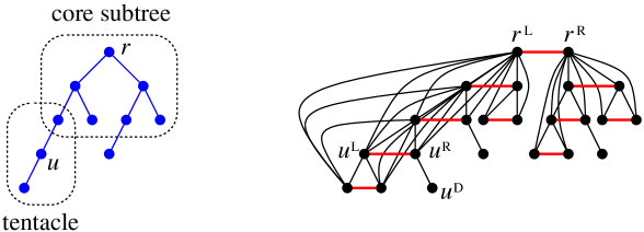
Figure 4: On the left, an example of a skeleton tree ${\cal T}$. The core subtree of ${\cal T}$ has depth $2$ and two tentacles, one of length $2$ and one of length $1$. On the right, the corresponding graph ${\cal G}$.

Skeleton-tree graphs.

The graph represented by a skeleton tree ${\cal T}$ will be denoted by ${\cal G}$. We differentiate between the nodes of ${\cal T}$ and the vertices of ${\cal G}$. The relation between ${\cal T}$ and ${\cal G}$ is illustrated in Figure 4. The graph ${\cal G}$ is obtained from the tree ${\cal T}$ as follows:

• For each node $u\in{\cal T}$ we create two vertices $u^{\mbox{\tiny\rm L}}$ and $u^{\mbox{\tiny\rm R}}$ in ${\cal G}$, with an edge between them. This edge $(u^{\mbox{\tiny\rm L}},u^{\mbox{\tiny\rm R}})$ is called the cross edge corresponding to $u$.

• Suppose that $u,v\in{\cal T}$. If $u$ is in the left subtree of $v$ then $(u^{\mbox{\tiny\rm L}},v^{\mbox{\tiny\rm L}})$ and $(u^{\mbox{\tiny\rm R}},v^{\mbox{\tiny\rm L}})$ are edges of ${\cal G}$. If $u$ is in the right subtree of $v$ then $(u^{\mbox{\tiny\rm L}},v^{\mbox{\tiny\rm R}})$ and $(u^{\mbox{\tiny\rm R}},v^{\mbox{\tiny\rm R}})$ are edges of ${\cal G}$. These edges are called upward edges.

• If $u\in{\cal T}$ is a node in a tentacle of ${\cal T}$ and is not a leaf of ${\cal T}$, then ${\cal G}$ has a vertex $u^{\mbox{\tiny\rm D}}$ with edge $(u^{\mbox{\tiny\rm D}},u^{\mbox{\tiny\rm R}})$. This edge is called a whisker.

The adversary strategy.

The adversary constructs ${\cal T}$ and ${\cal G}$ gradually, in response to strategy ${\cal S}$’s choices. Initially, ${\cal T}$ is a single node $r$, and thus ${\cal G}$ is a single edge $(r^{\mbox{\tiny\rm L}},r^{\mbox{\tiny\rm R}})$. At this time, $\mbox{\sf{profit}}_{\cal S}({\cal T})=0$ and $\mbox{\sf{profit}}_{{\scriptstyle\sf OPT}}({\cal T})=1$, so ${\cal S}$ is forced to collect this edge (that is, it creates a $2$-clique ${\left\{r^{\mbox{\tiny\rm L}},r^{\mbox{\tiny\rm R}}\right\}}$), since otherwise the adversary can immediately stop with unbounded absolute competitive ratio.

In general, the invariant of the construction is that, at each step, the only non-singleton cliques that ${\cal S}$ can add to its clustering are cross edges that correspond to the current leaves of ${\cal T}$. Suppose that, at some step, ${\cal S}$ collects a cross edge $(u^{\mbox{\tiny\rm L}},u^{\mbox{\tiny\rm R}})$, corresponding to node $u$ of ${\cal T}$. (${\cal S}$ may collect more cross edges in one step; if so, the adversary applies its strategy to each such edge independently.) If $u$ is at depth less than $D$, the adversary extends ${\cal T}$ by adding two children of $u$. If $u$ is at depth at least $D$, the adversary only adds the left child of $u$, thus extending the tentacle ending at $u$. In terms of ${\cal G}$, the first move appends two triangles to $u^{\mbox{\tiny\rm L}}$ and $u^{\mbox{\tiny\rm R}}$, with all corresponding upward edges. The second move appends a triangle to $u^{\mbox{\tiny\rm L}}$ and a whisker to $u^{\mbox{\tiny\rm R}}$ (see Figure 5). In the case when ${\cal S}$ decides not to collect any cross edges at some step, the adversary stops the process.

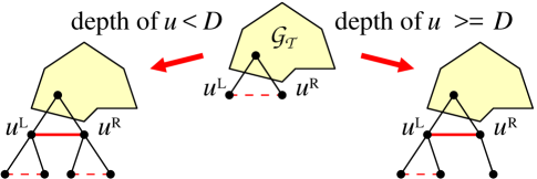
Figure 5: Adversary moves. Upward edges from new vertices are not shown, to avoid clutter. Dashed lines represent cross edges that are not collected by ${\cal S}$, while thick lines represent those that are already collected by ${\cal S}$.

Thus the adversary will be building the core binary skeleton tree down to depth $D$, and from then on, if the game still continues, it will extend the tentacles. Our objective is to prove that, in each step, right after the adversary extends the graph but before ${\cal S}$ updates its clustering, we have

$$\mbox{\sf{profit}}_{{\scriptstyle\sf OPT}}({\cal T})\geq(6-\epsilon_{D})\cdot\mbox{\sf{profit}}_{\cal S}({\cal T}),$$ (18)

where $\epsilon_{D}\to 0$ when $D\to\infty$. This is enough to prove the lower bound of $6-\epsilon_{D}$ on the absolute ratio. The reason is this: If ${\cal S}$ does not collect any edges at some step, the game stops, the ratio is $6-\epsilon_{D}$, and we are done. Otherwise, the adversary will stop the game after $2^{D+1}+M$ steps, where $M$ is some large integer. Then the profit of ${\cal S}$ is bounded by $2^{D+1}+M$ (the number of steps) plus the number of remaining cross edges, and there are at most $2^{D}$ of those, so ${\cal S}$’s profit is at most $2^{D+2}+M$. At that time, ${\cal T}$ will have at least $M$ nodes in tentacles and at most $2^{D}$ tentacles, so there is at least one tentacle of length $M/2^{D}$, and this tentacle contributes $\Omega((M/2^{D})^{2})$ edges to the optimum. Thus for $M$ large enough, the ratio between the optimal profit and the profit of ${\cal S}$ will be larger than $6$ (or any constant, in fact).

Once we establish (18), the lower bound of $6$ will follow, because for any fixed $R<6$ we can take $D$ large enough to get a lower of $6-\epsilon_{D}\geq R$.

Computing the adversary’s profit.

We now explain how to estimate the adversary’s profit for ${\cal G}$. To this end, we provide a specific recipe for computing a clique clustering of ${\cal G}$. We do not claim that this particular clustering is actually optimal, but it is a lower bound on the optimum profit, and thus it is sufficient for our purpose.

For any node $v\in{\cal T}$ that is not a leaf, denote by ${\cal P}^{\mbox{\tiny\rm L}}(v)$ the longest path from $v$ to a leaf of ${\cal T}$ that goes through the left child of $v$. If $v$ is a non-leaf in the core tree, and thus has a right child, then ${\cal P}^{\mbox{\tiny\rm R}}(v)$ is the longest path from $v$ to a leaf of ${\cal T}$ that goes through this right child. In both cases, ties are broken arbitrarily but consistently, for example in favor of the leftmost leaves. If $v$ is in a tentacle (so it does not have the right child), then we let ${\cal P}^{\mbox{\tiny\rm R}}(v)={\left\{v\right\}}$.

Let ${\cal P}^{\mbox{\tiny\rm L}}(v)=(v=v_{1},v_{2},...,v_{m})$, where $v_{m}$ is a leaf of ${\cal T}$. Since $v$ is not a leaf, the definition of ${\cal T}$ implies that $m\geq 2$. We now define the clique $C^{\mbox{\tiny\rm L}}(v)$ in ${\cal G}$ that corresponds to ${\cal P}^{\mbox{\tiny\rm L}}(v)$. Intuitively, for each $v_{i}$ we add to $C^{\mbox{\tiny\rm L}}(v)$ one of the corresponding vertices, $v_{i}^{\mbox{\tiny\rm L}}$ or $v_{i}^{\mbox{\tiny\rm R}}$, depending on whether $v_{i+1}$ is the left or to the right child of $v_{i}$. The following formal definition describes the construction of $C^{\mbox{\tiny\rm L}}(v)$ in a top-down fashion:

• $v_{1}^{\mbox{\tiny\rm L}}\in C^{\mbox{\tiny\rm L}}(v)$.

• Suppose that $1\leq i\leq m-1$ and that $v_{i}^{\sigma}\in C^{\mbox{\tiny\rm L}}(v)$, for $\sigma\in{\left\{{\mbox{\rm L}},{\mbox{\rm R}}\right\}}$. Then

  • if $i=m-1$, add $v_{m}^{\mbox{\tiny\rm L}}$ and $v_{m}^{\mbox{\tiny\rm R}}$ to $C^{\mbox{\tiny\rm L}}(v)$;

  • otherwise, if $v_{i+2}$ is the left child of $v_{i+1}$, add $v_{i+1}^{\mbox{\tiny\rm L}}$ to $C^{\mbox{\tiny\rm L}}(v)$, and if $v_{i+2}$ is the right child of $v_{i+1}$, add $v_{i+1}^{\mbox{\tiny\rm R}}$ to $C^{\mbox{\tiny\rm L}}(v)$.

We define $C^{\mbox{\tiny\rm R}}(v)$ analogously to $C^{\mbox{\tiny\rm L}}(v)$, but with two differences. One, we use ${\cal P}^{\mbox{\tiny\rm R}}(v)$ instead of ${\cal P}^{\mbox{\tiny\rm L}}(v)$. Two, if $v$ is in a tentacle then we let $C^{\mbox{\tiny\rm R}}(v)={\left\{v^{\mbox{\tiny\rm R}},v^{\mbox{\tiny\rm D}}\right\}}$. In other words, the whiskers form 2-cliques.

Observe that except cliques $C^{\mbox{\tiny\rm R}}(v)$ corresponding to the whiskers (that is, when $v$ is in a tentacle), all cliques $C^{\sigma}(v)$ have cardinality at least $3$.

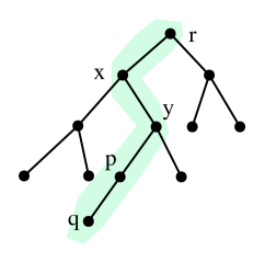
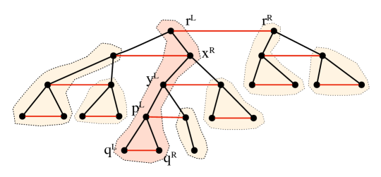
Figure 6: On the left, an example of a path ${\cal P}^{\mbox{\tiny\rm L}}(r)=(r,x,y,p,q)$ in ${\cal T}$. In this example, $D=3$. The corresponding clique $C^{\mbox{\tiny\rm L}}(r)$ is shown on the right (darker shape). The figure on the right also shows the adversary clique partitioning of ${\cal G}$. To avoid clutter, upward edges are not shown.

We now define a clique partitioning ${\cal C}^{\ast}$ of ${\cal G}$, as follows: First we include cliques $C^{\mbox{\tiny\rm L}}(r)$ and $C^{\mbox{\tiny\rm R}}(r)$ in ${\cal C}^{\ast}$. We then proceed recursively: choose any node $v$ such that exactly one of $v^{\mbox{\tiny\rm L}},v^{\mbox{\tiny\rm R}}$ is already covered by some clique of ${\cal C}^{\ast}$. If $v^{\mbox{\tiny\rm L}}$ is covered but $v^{\mbox{\tiny\rm R}}$ is not, then include $C^{\mbox{\tiny\rm R}}(v)$ in ${\cal C}^{\ast}$. Similarly, if $v^{\mbox{\tiny\rm R}}$ is covered but $v^{\mbox{\tiny\rm L}}$ is not, then include $C^{\mbox{\tiny\rm L}}(v)$ in ${\cal C}^{\ast}$.

Analysis.

Denote by ${\cal T}_{v}$ the subtree of ${\cal T}$ rooted at $v$. By ${\cal G}_{v}$ we denote the subgraph of ${\cal G}$ induced by the vertices that correspond to the nodes in ${\cal T}_{v}$. Each clique in ${\cal C}^{\ast}$ that intersects ${\cal G}_{v}$ induces a clique in ${\cal G}_{v}$, and the partitioning ${\cal C}^{\ast}$ induces a partitioning ${\cal C}^{\ast}_{v}$ of ${\cal G}_{v}$ into cliques. We will use notation $\mbox{\sf{O}}_{v}$ for the profit of partitioning ${\cal C}^{\ast}_{v}$. Note that ${\cal C}^{\ast}_{v}$ can be obtained with the same top-down process as ${\cal C}^{\ast}$, but starting from $v$ as the root instead of $r$.

We denote strategy ${\cal S}$’s profit (the number of cross edges) within ${\cal G}_{v}$ by $\mbox{\sf{S}}_{v}$ . In particular, we have $\mbox{\sf{profit}}_{\cal S}({\cal G})=\mbox{\sf{S}}_{r}$ and $\mbox{\sf{profit}}_{{\scriptstyle\sf OPT}}({\cal G})\geq\mbox{\sf{O}}_{r}$. Thus, to show (18), it is sufficient to prove that

$$\mbox{\sf{O}}_{r}\geq(6-\epsilon_{D})\cdot\mbox{\sf{S}}_{r},$$ (19)

where $\epsilon_{D}\to 0$ when $D\to\infty$.

We will in fact prove an analogue of inequality (19) for all subtrees ${\cal T}_{v}$. To this end, we distinguish between two types of subtrees ${\cal T}_{v}$. If ${\cal T}_{v}$ ends at depth $D$ of ${\cal T}$ or less (in other words, if ${\cal T}_{v}$ is inside the core of ${\cal T}$), we call ${\cal T}_{v}$ shallow. If ${\cal T}_{v}$ ends at depth $D+1$ or more, we call it deep. So deep subtrees are those that contain some tentacles of ${\cal T}$.

Lemma 3.3

If ${\cal T}_{v}$ is shallow, then

$$\mbox{\sf{O}}_{v}\geq 6\cdot\mbox{\sf{S}}_{v}.$$

Proof: This can be shown by induction on the depth of ${\cal T}_{v}$. If this depth is $0$, that is ${\cal T}_{v}={\left\{v\right\}}$, then $\mbox{\sf{O}}_{v}=1$ and $\mbox{\sf{S}}_{v}=0$, so the ratio is actually infinite. To jump-start the induction we also need to analyze the case when the depth of ${\cal T}_{v}$ is $1$. This means that ${\cal S}$ collected only edge $(v^{\mbox{\tiny\rm L}},v^{\mbox{\tiny\rm R}})$ from ${\cal T}_{v}$. When this happened, the adversary generated vertices corresponding to the two children of $v$ in ${\cal T}$ and his clustering will consist of two triangles. So now $\mbox{\sf{O}}_{v}=6$ and $\mbox{\sf{S}}_{v}=1$, and the lemma holds.

Inductively, suppose that the depth of ${\cal T}_{v}$ is at least two, let $y,z$ be the left and right children of $v$ in ${\cal T}$, and assume that the lemma holds for ${\cal T}_{y}$ and ${\cal T}_{z}$. Naturally, we have $\mbox{\sf{S}}_{v}=\mbox{\sf{S}}_{y}+\mbox{\sf{S}}_{z}+1$. Regarding the adversary profit, since the depth of ${\cal T}_{v}$ is at least two, cluster $C^{\mbox{\tiny\rm L}}(v)$ contains exactly one of $y^{\mbox{\tiny\rm L}},y^{\mbox{\tiny\rm R}}$; say it contains $y^{\mbox{\tiny\rm L}}$. Thus $C^{\mbox{\tiny\rm L}}(v)$ is obtained from $C^{\mbox{\tiny\rm L}}(y)$ by adding $v^{\mbox{\tiny\rm L}}$. By the definition of clustering ${\cal C}^{\ast}$, the depth of ${\cal T}_{y}$ is at least $1$, which means that adding $v^{\mbox{\tiny\rm L}}$ will add at least three new edges. By a similar argument, we will also add at least three edges from $v^{\mbox{\tiny\rm R}}$. This implies that $\mbox{\sf{O}}_{v}\geq\mbox{\sf{O}}_{y}+\mbox{\sf{O}}_{z}+6\geq 6\cdot\mbox{\sf{S}}_{y}+6\cdot\mbox{\sf{S}}_{z}+6\geq 6\cdot\mbox{\sf{S}}_{v}$, completing the inductive step. $\Box$

From Lemma (3.3) we obtain that, in particular, if ${\cal T}$ itself is shallow then $\mbox{\sf{O}}_{r}\geq 6\cdot\mbox{\sf{S}}_{r}$, which is even stronger than inequality (19) that we are in the process of justifying. Thus, for the rest of the proof, we can restrict our attention to skeleton trees ${\cal T}$ that are deep.

So next we consider deep subtrees of ${\cal T}$. The core depth of a deep subtree ${\cal T}_{v}$ is defined as the depth of the part of ${\cal T}_{v}$ within the core subtree of ${\cal T}$. (In other words, the core depth of ${\cal T}_{v}$ is equal to $D$ minus the depth of $v$ in ${\cal T}$.) If $h$ and $s$ are, respectively, the core depth of ${\cal T}_{v}$ and its maximum tentacle length, then $0\leq h\leq D$ and $s\geq 1$. The sum $h+s$ is then simply the depth of ${\cal T}$.

Lemma 3.4

Let ${\cal T}_{v}$ be a deep subtree of core depth $h\geq 0$ and maximum tentacle length $s\geq 1$, then

$$\mbox{\sf{O}}_{v}+2(h+s)\geq 6\cdot\mbox{\sf{S}}_{v}.$$

Before proving the lemma, let us argue first that this lemma is sufficient to establish our lower bound. Indeed, since we are now considering the case when ${\cal T}$ is a deep subtree itself, the lemma implies that $\mbox{\sf{O}}_{r}+2(D+s)\geq 6\cdot\mbox{\sf{S}}_{r}$, where $s$ is the maximum tentacle length of ${\cal T}$. But $\mbox{\sf{O}}_{r}$ is at least quadratic in $D+s$. So for large $D$ the ratio $\mbox{\sf{O}}_{r}/\mbox{\sf{S}}_{r}$ approaches $6$.

Proof: To prove Lemma 3.4, we use induction on $h$, the core depth of ${\cal T}_{v}$. Consider first the base case, for $h=0$ (when ${\cal T}_{v}$ is just a tentacle). In his clustering ${\cal C}^{\ast}_{v}$, the adversary has one clique of $s+2$ vertices, namely all $x^{\mbox{\tiny\rm L}}$ vertices in the tentacle (there are $s+1$ of these), plus one $z^{\mbox{\tiny\rm R}}$ vertex for the leaf $z$. He also has $s$ whiskers, so his profit for ${\cal T}_{v}$ is $\binom{s+2}{2}+s={\textstyle\frac{1}{2}}(s^{2}+5s+2)$. ${\cal S}$ collects only $s$ edges, namely all cross edges in ${\cal T}_{v}$ except the last. (See Figure 7.) Solving the quadratic inequality and using the integrality of $s$, we get $\mbox{\sf{O}}_{v}+2s\geq 6s=6\cdot\mbox{\sf{S}}_{v}$. Note that this inequality is in fact tight for $s=1$ and $2$.

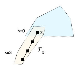
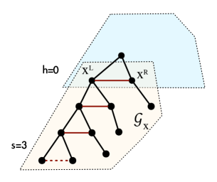
Figure 7: Illustration of the proof of Lemma 3.4, the base case. Subtree ${\cal T}_{v}$ on the left, the corresponding subgraph ${\cal G}_{v}$ on the right.

In the inductive step, consider a deep subtree ${\cal T}_{v}$. Let $y$ and $z$ be the left and right children of $v$. Without loss of generality, we can assume that ${\cal T}_{y}$ is a deep tree with core depth $h-1$ and the same maximum tentacle length $s$ as ${\cal T}_{v}$, while ${\cal T}_{z}$ is either shallow (that is, it has no tentacles), or it is a deep tree with maximum tentacle length at most $s$.

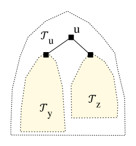
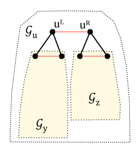
Figure 8: Illustration of the proof of Lemma 3.4, the inductive step. Subtrees ${\cal T}_{v},{\cal T}_{y},{\cal T}_{z}$ on the left, the corresponding subgraphs on the right.

By the inductive assumption, we have $\mbox{\sf{O}}_{y}+2(h-1+s)\geq 6\cdot\mbox{\sf{S}}_{y}$. Regarding $z$, if ${\cal T}_{z}$ is shallow then from Lemma 3.3 we get $\mbox{\sf{O}}_{z}\geq 6\cdot\mbox{\sf{S}}_{z}$, and if ${\cal T}_{z}$ is deep (necessarily of core depth $h-1$) then $\mbox{\sf{O}}_{z}+2(h-1+s^{\prime})\geq 6\cdot\mbox{\sf{S}}_{z}$, where $s^{\prime}$ is ${\cal T}_{z}$’s maximum tentacle length, such that $1\leq s^{\prime}\leq s$.

Consider first the case when ${\cal T}_{z}$ is shallow. Note that

$$\mbox{\sf{S}}_{v} =\mbox{\sf{S}}_{y}+\mbox{\sf{S}}_{z}+1\ \ \mbox{and}$$

$$\mbox{\sf{O}}_{v} \geq\mbox{\sf{O}}_{y}+\mbox{\sf{O}}_{z}+h+s+4$$

The first equation is trivial, because the profit of ${\cal S}$ in ${\cal G}_{v}$ consists of all cross edges in ${\cal G}_{y}$ and ${\cal G}_{z}$, plus one more cross edge $(v^{\mbox{\tiny\rm L}},v^{\mbox{\tiny\rm R}})$. The second inequality holds because the adversary clustering ${\cal C}^{\ast}_{v}$ is obtained by adding $v^{\mbox{\tiny\rm L}}$ to ${\cal G}_{y}$’s cluster with $(h-1)+s+2=h+s+1$ vertices, and $v^{\mbox{\tiny\rm R}}$ can be added to ${\cal G}_{z}$’s cluster that with at least $3$ vertices. We get

$$\mbox{\sf{O}}_{v}+2(h+s) \geq[\mbox{\sf{O}}_{y}+\mbox{\sf{O}}_{z}+h+s+4]+2(h+s)$$

$$\geq[\mbox{\sf{O}}_{y}+2(h-1+s)]+\mbox{\sf{O}}_{z}+6$$

$$\geq 6\cdot\mbox{\sf{S}}_{y}+6\cdot\mbox{\sf{S}}_{z}+6$$

$$=6\cdot\mbox{\sf{S}}_{v}.$$

The second case is when ${\cal T}_{z}$ is a deep tree (of the same core depth $h-1$ as ${\cal T}_{y}$) with maximum tentacle length $s^{\prime}$, where $1\leq s^{\prime}\leq s$. As before, we have $\mbox{\sf{S}}_{v}=\mbox{\sf{S}}_{y}+\mbox{\sf{S}}_{z}+1$. The optimum profit satisfies (by a similar argument as before, applied to both ${\cal T}_{y}$ and ${\cal T}_{z}$)

$$\mbox{\sf{O}}_{v} \geq\mbox{\sf{O}}_{y}+\mbox{\sf{O}}_{z}+2h+s+s^{\prime}+2.$$

We obtain (using $s\geq s^{\prime}$)

$$\mbox{\sf{O}}_{v}+2(h+s) \geq[\mbox{\sf{O}}_{y}+\mbox{\sf{O}}_{z}+2h+s+s^{\prime}+2]+2(h+s)$$

$$\geq[\mbox{\sf{O}}_{y}+2(h-1+s)]+[\mbox{\sf{O}}_{z}+2(h-1+s^{\prime})]+6$$

$$\geq 6\cdot\mbox{\sf{S}}_{y}+6\cdot\mbox{\sf{S}}_{z}+6$$

$$=6\cdot\mbox{\sf{S}}_{v}.$$

This completes the proof of Lemma 3.4. $\Box$

We still need to explain how to extend our proof so that it also applies to the asymptotic competitive ratio. This is quite simple: Choose some large constant $K$. The adversary will create $K$ instances of the above game, playing each one independently. Our construction above uses the fact that at each step the strategy is forced to collect one of the pending cross edges, otherwise its competitive ratio exceeds ratio $R$ (where $R$ is arbitrarily close to $6$). Now, for $K$ sufficiently large, the strategy is forced to collect cross edges in all except for some finite number of copies of the game, where this number depends on the additive constant in the competitiveness bound.

Note: Our construction is very tight, in the following sense. Suppose that ${\cal S}$ maintains ${\cal T}$ as balanced as possible. Then the ratio is exactly $6$ when the depth of ${\cal T}$ is $1$ or $2$. Furthermore, suppose that $D$ is very large and the strategy constructs ${\cal T}$ to have depth $D$ or more, that is, it starts growing tentacles (but still maintaining ${\cal T}$ balanced.) Then the ratio is $6-o(1)$ for tentacle lengths $s=1$ and $s=2$. The intuition is that when the adversary plays optimally, he will only allow the online strategy to collect isolated edges (cliques of size $2$). For this reason, we conjecture that $6$ is the optimal competitive ratio.

4 Online MinCC Clustering

In this section, we study the clique clustering problem with a different measure of optimality that we call MinCC. For MinCC, we define the cost of a clustering ${\cal C}$ to be the total number of non-cluster edges. Specifically, if the cliques in ${\cal C}$ are $C_{1},C_{2},...,C_{k}$ then the cost of ${\cal C}$ is $|E|-\sum_{i=1}^{k}\binom{|C_{i}|}{2}$. The objective is to construct a clustering that minimizes this cost.

4.1 A Lower Bound for Online MinCC Clustering

In this section we present a lower bound for deterministic MinCC clustering.

Theorem 4

(a) There is no online strategy for MinCC clustering with competitive ratio $n-\omega(1)$, where $n$ is the number of vertices.

(b) There is no online strategy for MinCC clustering with absolute competitive ratio smaller than $n-2$.

Proof: (a) Consider a strategy ${\cal S}$ with competitive ratio $R_{n}=n-\omega(1)$. Thus, according to the definition (2) of the competitive ratio, there is a constant $\beta$ that satisfies $\mbox{\sf{cost}}_{{\cal S}}(G)\leq R_{n}\cdot\mbox{\sf{cost}}_{\scriptstyle\sf OPT}(G)+\beta$, where $n=|G|$. We can assume that $\beta$ is a positive integer.

Figure 9: Illustrating the lower bound proof of Theorem 4. The figure shows the optimal clustering for the graph.

The adversary first produces a graph of $2\beta+2$ vertices connected by $\beta+1$ disjoint edges $(v_{2i-1},v_{2i})$, for $i=1,2,\ldots,\beta+1$. At this point, ${\cal S}$ must have added at least one pair ${\left\{v_{2j-1},v_{2j}\right\}}$ to its clustering, because otherwise, since $\mbox{\sf{cost}}_{\scriptstyle\sf OPT}(G)=0$, inequality (2) would be violated. The adversary then chooses some large $n$ and adds $n-2\beta-2$ new vertices $v_{2\beta+3},\ldots,v_{n}$ that together with $v_{2j}$ form a clique of size $n-2\beta-1$; see Figure 9. All edges from $v_{2j}$ to these new vertices are non-cluster edges for ${\cal S}$ and the optimum solution has only one non-cluster edge $(v_{2j-1},v_{2j})$. Thus

$$\mbox{\sf{cost}}_{{\cal S}}(G)-\beta\geq(n-2\beta-2)-\beta=n-3\beta-2=(n-3\beta-2)\cdot\mbox{\sf{cost}}_{\scriptstyle\sf OPT}(G)>R_{n}\cdot\mbox{\sf{cost}}_{\scriptstyle\sf OPT}(G),$$

if $n$ is large enough, giving us a contradiction.

(b) The proof of this part is a straightforward modification of the proof for (a): the adversary starts by releasing just one edge $(v_{1},v_{2})$, and the online strategy is forced to cluster $v_{1}$ and $v_{2}$ together, because now $\beta=0$. Then the adversary forms a clique of size $n-1$ including $v_{2}$. The details are left to the reader. $\Box$

4.2 The Greedy Strategy for Online MinCC Clustering

We continue the study of online MinCC clustering, and we prove that Greedy, the greedy strategy presented in Section 3.1, yields a competitive ratio matching the lower bound from the previous section.

Theorem 5

The absolute competitive ratio of Greedy is $n-2$.

Proof: The key observation for this proof is that, for any triplet of vertices $u$, $v$, and $v^{\prime}$, if the graph contains the two edges $(u,v)$ and $(u,v^{\prime})$ but $v$ and $v^{\prime}$ are not connected by an edge, then in any clustering at least one of the edges $(u,v)$ or $(u,v^{\prime})$ is a non-cluster edge.

Claim A: Let $(u,v)$ be a non-cluster edge of Greedy. Then OPT (the optimal clustering) has at least one non-cluster edge adjacent to $u$ or $v$ (which might also be $(u,v)$ itself).

Without loss of generality suppose vertex $v$ arrives after vertex $u$. Let $A$ be the cluster of Greedy containing vertex $u$ at the moment when vertex $v$ arrives. We have that $v\notin A$. If $A$ contains some vertex $u^{\prime}$ not connected to $v$, then the earlier key observation shows that one of the edges $(u^{\prime},u)$, $(u,v)$ is a non-cluster edge for OPT; see Figure 10.

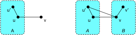
Figure 10: Illustration of the proof of Theorem 5.

Now assume that $v$ is connected to all vertices of $A$. Greedy had an option of adding $v$ to $A$ and it didn’t, so it placed $v$ in some clique $B$ (of size at least $2$) that is not merge-able with $A$, that is, there are vertices $u^{\prime}\in A$ and $v^{\prime}\in B$ which are not connected by an edge. Now the earlier key observation shows that one of the edges $(u^{\prime},v)$, $(v,v^{\prime})$ is a non-cluster edge of OPT. This completes the proof of Claim A.

To estimate the number of non-cluster edges of Greedy, we use a charging scheme. Let $(u,v)$ be a non-cluster edge of Greedy. We charge it to non-cluster edges of OPT as follows.

Self charge: If $(u,v)$ is a non-cluster edge of OPT, we charge $1$ to $(u,v)$ itself.

Proximate charge: If $(u,v)$ is a cluster edge in OPT, we split the charge of $1$ from $(u,v)$ evenly among all non-cluster edges of OPT incident to $u$ or $v$.

From Claim A, the charging scheme is well-defined, that is, all non-cluster edges of Greedy have been charged fully to non-cluster edges of OPT. It remains to estimate the total charge that any non-cluster edge of OPT may have received. Since the absolute competitive ratio is the ratio between the number of non-cluster edges of Greedy and the number of non-cluster edges of OPT, the maximum charge to any non-cluster edge of OPT is an upper bound for the absolute competitive ratio.

Consider a non-cluster edge $(x,y)$ of OPT. Edge $(x,y)$ can receive charges only from itself (self charge) and other edges incident to $x$ or $y$ (proximate charges). Let $P$ be the set of vertices adjacent to both $x$ and $y$, and let $Q$ be the set of vertices that are adjacent to only one of them, but excluding $x$ and $y$:

$$P=N(x)\cap N(y)\quad\textrm{and}\quad Q=N(x)\cup N(y)-P-{\left\{x,y\right\}}.$$

($N(z)$ denotes the neighborhood of a vertex $z$, the set of vertices adjacent to $z$.) We have $|P|+|Q|\leq n-2$.

Edges connecting $x$ or $y$ to $Q$ will be called $Q$-edges. Trivially, the total charge from $Q$-edges to $(x,y)$ is at most $|Q|$.

Edges connecting $x$ or $y$ to $P$ will be called $P$-edges. Consider some $z\in P$. Since $x$ and $y$ are in different clusters of OPT, at least one of $P$-edges $(x,z)$ or $(y,z)$ must also be a non-cluster edge for OPT. By symmetry, assume that $(x,z)$ is a non-cluster edge for OPT. If $(x,z)$ is a non-cluster edge of Greedy then $(x,z)$ will absorb its self charge. So $(x,z)$ will not contribute to the charge of $(x,y)$. If $(y,z)$ is a non-cluster edge of Greedy then either it will be self charged (if it’s also a non-cluster edge of OPT) or its proximate charge will be split between at least two edges, namely $(x,y)$ and $(x,z)$. Thus the charge from $(y,z)$ to $(x,y)$ will be at most ${\textstyle\frac{1}{2}}$. Therefore the total charge from $P$-edges to $(x,y)$ is at most ${\textstyle\frac{1}{2}}|P|$. We now have some cases.

Case 1: $(x,y)$ is a cluster edge of Greedy. Then $(x,y)$ does not generate a self charge, so the total charge received by $(x,y)$ is at most ${\textstyle\frac{1}{2}}|P|+|Q|\leq|P|+|Q|\leq n-2$.

Case 2: $(x,y)$ is a non-cluster edge of Greedy. Then $(x,y)$ contributes a self charge to itself.

Case 2.1: $|P|\geq 2$. Then ${\textstyle\frac{1}{2}}|P|\leq|P|-1$, so the total charge received by $(x,y)$ is at most ${\textstyle\frac{1}{2}}|P|+|Q|+1\leq(|P|-1)+|Q|=|P|+|Q|\leq n-2$.

Case 2.2: At least one $Q$-edge is a cluster edge of Greedy. Then the total proximate charge from $Q$-edges is at most $|Q|-1$, so the total charge received by $(x,y)$ is at most ${\textstyle\frac{1}{2}}|P|+(|Q|-1)+1\leq|P|+|Q|\leq n-2$.

Case 2.3: $|P|\in{\left\{0,1\right\}}$ and all $Q$-edges are non-cluster edges of Greedy. We claim that this case cannot actually occur. Indeed, if $|P|=0$ then Greedy would cluster $x$ and $y$ together. Similarly, if $P={\left\{z\right\}}$, then Greedy would cluster $x$, $y$ and $z$ together. In both cases, we get a contradiction with the assumption of Case 2.

Summarizing, we have shown that each non-cluster edge of OPT receives a total charge of at most $n-2$, and the theorem follows. $\Box$

The proof of Theorem 5 applies in fact to a more general class of strategies, giving an upper bound of $n-2$ on the absolute competitive ratio of all “non-procrastinating” strategies, which never leave merge-able clusters in their clusterings (that is clusters $C$, $C^{\prime}$ such that $C\cup C^{\prime}$ forms a clique).

References

- [1] Nikhil Bansal, Avrim Blum, and Shuchi Chawla. Correlation clustering. Machine Learning, 56(1-3):89–113, 2004.
- [2] Amir Ben-Dor, Ron Shamir, and Zohar Yakhini. Clustering gene expression patterns. Journal of Computational Biology, 6(3/4):281–297, 1999.
- [3] Allan Borodin and Ran El-Yaniv. Online computation and competitive analysis. Cambridge University Press, 1998.
- [4] Moses Charikar, Chandra Chekuri, Tomás Feder, and Rajeev Motwani. Incremental clustering and dynamic information retrieval. SIAM J. Comput., 33(6):1417–1440, 2004.
- [5] Moses Charikar, Venkatesan Guruswami, and Anthony Wirth. Clustering with qualitative information. In Foundations of Computer Science, 2003. Proceedings. 44th Annual IEEE Symposium on, pages 524–533. IEEE, 2003.
- [6] Kamalika Chaudhuri, Brighten Godfrey, Satish Rao, and Kunal Talwar. Paths, trees, and minimum latency tours. In 44th Symposium on Foundations of Computer Science (FOCS 2003), 11-14 October 2003, Cambridge, MA, USA, Proceedings, pages 36–45, 2003.
- [7] Marek Chrobak, Christoph Dürr, and Bengt J. Nilsson. Competitive strategies for online clique clustering. In Proc. 9th International Conference on Algorithms and Complexity (CIAC’15), pages 101–113, 2015.
- [8] Marek Chrobak and Mathilde Hurand. Better bounds for incremental medians. Theor. Comput. Sci., 412(7):594–601, 2011.
- [9] Marek Chrobak, Claire Kenyon, John Noga, and Neal E. Young. Incremental medians via online bidding. Algorithmica, 50(4):455–478, 2008.
- [10] Marek Chrobak and Claire Kenyon-Mathieu. SIGACT news online algorithms column 10: competitiveness via doubling. SIGACT News, 37(4):115–126, 2006.
- [11] Erik D. Demaine and Nicole Immorlica. Correlation clustering with partial information. In Proc. 6th International Workshop on Approximation Algorithms for Combinatorial Optimization Problems (APPROX’03), pages 1–13, 2003.
- [12] Anders Dessmark, Jesper Jansson, Andrzej Lingas, Eva-Marta Lundell, and Mia Persson. On the approximability of maximum and minimum edge clique partition problems. In Proceedings of the 12th Computing: The Australasian Theory Symposium (CATS’06), pages 101–105, 2006.
- [13] Aleksander Fabijan, Bengt J. Nilsson, and Mia Persson. Competitive online clique clustering. In Proc. 8th International Conference on Algorithms and Complexity (CIAC’13), pages 221–233, 2013.
- [14] Andres Figueroa, James Borneman, and Tao Jiang. Clustering binary fingerprint vectors with missing values for DNA array data analysis. Journal of Computational Biology, 11(5):887–901, 2004.
- [15] Andres Figueroa, Avraham Goldstein, Tao Jiang, Maciej Kurowski, Andrzej Lingas, and Mia Persson. Approximate clustering of incomplete fingerprints. J. Discrete Algorithms, 6(1):103–108, 2008.
- [16] Guolong Lin, Chandrashekhar Nagarajan, Rajmohan Rajaraman, and David P. Williamson. A general approach for incremental approximation and hierarchical clustering. SIAM J. Comput., 39(8):3633–3669, 2010.
- [17] Claire Mathieu, Ocan Sankur, and Warren Schudy. Online correlation clustering. In 27th International Symposium on Theoretical Aspects of Computer Science (STACS’10), pages 573–584, 2010.
- [18] Ron Shamir, Roded Sharan, and Dekel Tsur. Cluster graph modification problems. Discrete Applied Mathematics, 144(1-2):173–182, 2004.
- [19] Lea Valinsky, Gianluca Della Vedova, Ra J. Scupham, Sam Alvey, Andres Figueroa, Bei Yin, R. Jack Hartin, Marek Chrobak, David E. Crowley, Tao Jiang, and James Borneman. Analysis of bacterial community composition by oligonucleotide fingerprinting of rRNA genes. Applied and Environmental Microbiology, 68:2002, 2002.