E2-quasi-exact solvability for non-Hermitian models

Abstract:

We propose the notion of $E_{2}$-quasi-exact solvability and apply this idea to find explicit solutions to the eigenvalue problem for a non-Hermitian Hamiltonian system depending on two parameters. The model considered reduces to the complex Mathieu Hamiltonian in a double scaling limit, which enables us to compute the exceptional points in the energy spectrum of the latter as a limiting process of the zeros for some algebraic equations. The coefficient functions in the quasi-exact eigenfunctions are univariate polynomials in the energy obeying a three-term recurrence relation. The latter property guarantees the existence of a linear functional such that the polynomials become orthogonal. The polynomials are shown to factorize for all levels above the quantization condition leading to vanishing norms rendering them to be weakly orthogonal. In two concrete examples we compute the explicit expressions for the Stieltjes measure.

1 Introduction

In almost any study of quantum mechanical systems the determination of explicit and ideally exact solutions to the associated eigenvalue problem is either part of the key aims or at least essential ingredient. Integrability is a property that largely facilitates to achieve this goal. Prime examples for models that are integrable and can be solved exactly, classically as well as quantum mechanically, are Calogero [1, 2] and Sutherland models [3]. A systematic study of such type of models can be established by relating them to Lie algebraic structures [4, 5] and exploiting the fact that the eigenfunctions of some Hamiltonian systems form a flag which coincides with the finite dimensional representation space of the associated Lie algebras. Models of this type for which the representation space is finite are usually referred to as quasi-exactly solvable models [6, 7] of Lie algebraic type. Most of these models can be related to $sl_{2}(\mathbb{C})$ with their compact and non-compact real forms $su(2)$ and $su(1,1)$, respectively [8].

However, in the context of extending [9, 10] the study of such models to non-Hermitian models of quasi-Hermitian/$\mathcal{PT}$-symmetric type [11, 12, 13, 14] it was recently found [15] that a more natural setting for some systems is to cast them in terms of Euclidean Lie algebras. Support for using the latter algebras in some cases also comes from the actual solutions of the related eigenvalue problem, i.e. the fact that the eigenfunctions of $sl_{2}(\mathbb{C})$ related systems are usually hypergeometric functions or their reduced versions whereas the solutions of systems related Euclidean algebras are usually Mathieu functions. It is well known that due to their different singularity structure the two can not be related in the sense that one may express Mathieu functions in terms of hypergeometric functions or vice versa. Thus, systems of this type call for a different setting. Besides these more mathematical aspects, a special interest in such type of models results also from the fact that they are related to optical systems when reducing the Schrödinger equation to the Helmholtz equation. Concrete versions of complex potentials leading to real Mathieu potentials have recently been studied from a theoretical as well as experimental point of view in [16, 17, 18, 19, 20, 21, 22].

In the above spirit we suggest the general notion of $E_{2}$-quasi exact solvability in a quite analogue fashion when compared to $sl_{2}(\mathbb{C})$-solvability. The key difference is that we cast the Hamiltonian in terms of the generators of the Euclidean Lie algebra and also adapt the vector space on which they act accordingly. We apply the general idea to solve a model, which in a mildly modified version was first noted to be expressible in terms of $sl_{2}(\mathbb{C})$-generators by Khare and Mandal [23]. Making use of this quasi-exactly solvable structure the model was analyzed further by Bagchi, Quesne Mallik and Roychoudhury in [24, 25] for the lowest levels. In particular the authors exploited the double scaling limit towards the Mathieu equation and identified one exceptional point. By reformulating the problem in terms of an $E_{2}$-setting we are able to push this analysis further and provide a complete set of solutions which in principle allows to identify all exceptional points from the double scaling limit. We carry out the limit in two alternative ways, either on the basis of the level-by-level solutions or directly for the recursive equation itself and interpret the resulting equations as an eigenvalue problem for an infinite matrix. The latter approach leads to much faster convergence.

We demonstrate that also at the heart of this type of $E_{2}$-quasi exact solvability lies the fact the coefficient function polynomials in our eigenfunctions possess the same essential features as the Bender-Dunne polynomials [26], i.e. they obey a three-term recurrence relation which is reset at a certain level to a two-term relation with the consequence that they factorize at the levels above. When going “on-shell”, i.e. taking the energy to be quantized, one of the two factors vanishes. By Favard’s theorem [27] the three-term recurrence relation already guarantees the existence of a linear functional, such that the polynomials form an orthogonal set. However, the fact that some of the polynomials vanish “on-shell” makes them weakly orthogonal polynomials as defined in [28]. We determine the explicit form of the functional by computing the expressions of the Stieltjes measure. For many computations, such as the evaluation of the norm or the momentum functional, the explicit knowledge of the measure is not needed when one assumes the functional to exist and exploits the three-term recurrence relation. However, this possibility is restricted to specific computations. Whenever possible we use the two alternative ways to compute the same quantity to demonstrate self-consistency.

Our manuscript is organized as follows: Based on the Euclidean Lie algebra $E_{2}$ we propose in section 2 the notion of $E_{2}$-quasi-exact solvability. In section 3 we apply this idea to solve the eigenvalue problem for a non-Hermitian model that reduces to the complex Mathieu Hamiltonian in the double scaling limit. We determine the exceptional points of the latter in two alternative ways and provide a detailed analysis of the polynomial coefficient functions with regard to their weakly orthogonal structure. Our conclusions and a further outlook into open problems are stated in section 4.

2 $E_{2}$-quasi-exact solvability

We introduce $E_{2}$-quasi-exactly solvable models in complete analogy to the notion of $sl_{2}(\mathbb{C})$-quasi-exactly solvability originally proposed by Turbiner [6, 7]. For this one considers Hamiltonian operators $\mathcal{H}$ expressible in terms of $sl_{2}(\mathbb{C})$-generators acting on spaces $V_{n}$ of polynomials of order $n$ as $\mathcal{H}:V_{n}\mapsto V_{n}$ preserving the flag structure $V_{0}\subset V_{1}\subset V_{2}\subset\ldots\subset V_{n}\subset\ldots$Whenever the first eigenvalues and eigenfunctions of this sequence can be found the models are referred to as quasi-exactly solvable, whereas when the entire infinite flag is preserved they are called exactly solvable. Integrability is conceptually different, but often related [4, 5]. Here we express the Hamiltonians in terms of $E_{2}$-Lie algebraic generators and proceed in a similar fashion.

The Euclidean algebra $E_{2}$ is the Lie algebra associated to the group $E(2)$ describing Euclidean transformations in the plane. We recall the commutation relations obeyed by its three generators $u$, $v$ and $J$

$$\left[u,J\right]=iv,\qquad\left[v,J\right]=-iu,\qquad\text{and\qquad}\left[u,v\right]=0.$$ (1)

There are various useful representation for this algebra. We denote by $\Pi^{(1)}$ the one acting on square integrable wavefunctions $L^{2}(\mathbf{S}^{1},d\theta)$

$$\Pi^{(1)}:\quad J:=-i\partial_{\theta},\quad u:=\sin\theta,\quad v:=\cos\theta,$$ (2)

employed for instance in the context of quantizing strings on tori [29]. The Casimir operator $C=u^{2}+v^{2}$ is here set to $1$. In Cartesian coordinates the corresponding representations are for instance

$$\Pi^{(2)} : \quad J:=yp_{x}-xp_{y},\quad u:=x,\quad~{}v:=y,$$ (3)

$$\Pi^{(3)} : \quad J:=xp_{y}-p_{x}y,\quad u:=p_{y},\quad v:=p_{x},$$ (4)

where $x,y,p_{x},p_{y}$ are the Heisenberg canonical variables $x,y,p_{x},p_{y}$ with non-vanishing commutators $\left[x,p_{x}\right]=\left[y,p_{y}\right]=i$ in the convention $\hbar=1$. The constraint for (3) and (4) on the Casimir operator is viewed in coordinate space as $x^{2}+y^{2}=1$ or momentum space as $p_{x}^{2}+p_{y}^{2}=1$, respectively.

In [15] five different types of anti-linear (or $\mathcal{PT}$) symmetries for the $E_{2}$-algebra were identified. Adopting the notation from there we are here especially interested in the symmetry $\mathcal{PT}_{3}:J\rightarrow J$, $u\rightarrow v$, $v\rightarrow u$, $i\rightarrow-i$, as this one is also respected by the model considered below. For our concrete representations this translates into $\mathcal{PT}_{3}^{\Pi^{(1)}}:\theta\rightarrow\pi/2-\theta$, $i\rightarrow-i$, $\mathcal{PT}_{3}^{\Pi^{(2)}}:x\rightarrow y$, $y\rightarrow x$, $p_{x}\rightarrow-p_{y}$, $p_{y}\rightarrow-p_{x}$, $i\rightarrow-i$, and $\mathcal{PT}_{3}^{\Pi^{(3)}}:x\rightarrow-y$, $y\rightarrow-x$, $p_{x}\rightarrow p_{y}$, $p_{y}\rightarrow p_{x}$, $i\rightarrow-i$. For the representation $\Pi^{(1)}$ we now define two $\mathcal{PT}_{3}^{\Pi^{(1)}}$-invariant vector spaces over $\mathbb{R}$ as follows

$$V_{n}^{s}(\phi_{0}) : =\mathop{\mathrm{s}pan}\left\{\left.\phi_{0}\left[\sin(2\theta),i\sin(4\theta),\ldots,i^{n+1}\sin(2n\theta)\right]\right|\theta\in\mathbb{R},\mathcal{PT}_{3}(\phi_{0})=\phi_{0}\in L\right\},~{}~{}~{}~{}~{}~{}$$ (5)

$$V_{n}^{c}(\phi_{0}) : =\mathop{\mathrm{s}pan}\left\{\left.\phi_{0}\left[1,i\cos(2\theta),\ldots,i^{n}\cos(2n\theta)\right]\right|\theta\in\mathbb{R},\mathcal{PT}_{3}(\phi_{0})=\phi_{0}\in L\right\}.$$ (6)

Evidently we have $\mathcal{PT}_{3}^{\Pi^{(1)}}:\psi\rightarrow\psi$ for all $\psi\in V_{n}^{s,c}(\phi_{0})$. Next we compute the action of some $\mathcal{PT}_{3}$-invariant combinations of $E_{2}$-generators on these spaces for concrete choices of $\phi_{0}$, which will turn out to be the ground state wavefunction. Let us take $\phi_{0}^{c}=e^{i\kappa\cos 2\theta}$ and $\phi_{0}^{s}=e^{\kappa\sin 2\theta}$ with $\kappa\in\mathbb{R}$. Then we find

$$J : V_{n}^{s,c}\left(\phi_{0}^{c}\right)\mapsto V_{n+1}^{c,s}\left(\phi_{0}^{c}\right),$$ (7)

$$uv : V_{n}^{s,c}\left(\phi_{0}^{c}\right)\mapsto V_{n+1}^{c,s}\left(\phi_{0}^{c}\right),$$ (8)

$$i(u^{2}-v^{2}) : V_{n}^{s,c}\left(\phi_{0}^{c}\right)\mapsto V_{n+1}^{s,c}\left(\phi_{0}^{c}\right),$$ (9)

and

$$J : V_{n}^{s,c}\left(\phi_{0}^{s}\right)\mapsto V_{n}^{c,s}\left(\phi_{0}^{s}\right)\oplus V_{n+1}^{s,c}\left(\phi_{0}^{s}\right),$$ (10)

$$uv : V_{n}^{s,c}\left(\phi_{0}^{s}\right)\mapsto V_{n+1}^{c,s}\left(\phi_{0}^{s}\right),$$ (11)

$$i(u^{2}-v^{2}) : V_{n}^{s,c}\left(\phi_{0}^{s}\right)\mapsto V_{n+1}^{s,c}\left(\phi_{0}^{s}\right).$$ (12)

The actions of other invariant combinations, such as $i(v-u)$ and $v+u$, may of course also be considered, but they do not map the spaces $V_{n}^{s,c}(\phi_{0}^{s,c})$ into each other. One may also include the possibility to have odd integer coefficient for $\theta$ in the arguments of the trigonometric functions in $V_{n}^{s,c}(\phi_{0})$. However, these versions are more complicated and the two spaces start to mix when acted upon with the $E_{2}$-generators.

Clearly this analysis should not be representation dependent and of course one can transform $V_{n}^{s}(\phi_{0})$, $V_{n}^{c}(\phi_{0})$ and the above arguments directly into the representations $\Pi^{(2,3)}$. Proceeding in a one-to-one fashion would involve a span over symmetric polynomials in $x,y$ or $p_{x},p_{y}$, which is not obvious to guess if one does not make a reference to representation $\Pi^{(1)}$. However, due to the constraint on the Casimir operator one may trade all even powers in one variable for the other and work with a simplified versions of polynomials in just one variable. Thus for $\Pi^{(2)}$ we define the vector spaces

$$\hat{V}_{n}^{s}(\phi_{0}) : =\mathop{\mathrm{s}pan}\left\{\left.\phi_{0}\left(xy,x^{3}y,\ldots,x^{2n+1}y\right)\right|x\in\mathbb{R},\mathcal{PT}_{3}(\phi_{0})=\phi_{0}\in L\right\},~{}~{}~{}~{}~{}~{}$$ (13)

$$\hat{V}_{n}^{c}(\phi_{0}) : =\mathop{\mathrm{s}pan}\left\{\left.\phi_{0}\left(1,x^{2},\ldots,x^{2n}\right)\right|\theta\in\mathbb{R},\mathcal{PT}_{3}(\phi_{0})=\phi_{0}\in L\right\}.$$ (14)

As a consequence of our replacements $y^{2n}\rightarrow(1-x^{2})^{n}$ we have lost the explicit $\mathcal{PT}_{3}$-symmetry and must span the vector space over $\mathbb{C}$ in this case. Taking now $\phi_{0}^{c}=e^{i\kappa(y^{2}-x^{2})}$ and $\phi_{0}^{s}=e^{\kappa xy}$ with $\kappa\in\mathbb{R}$ we find

$$J,uv : \hat{V}_{n}^{c}\left(\phi_{0}^{c}\right)\mapsto\hat{V}_{n}^{s}\left(\phi_{0}^{c}\right),$$ (15)

$$J,uv : \hat{V}_{n}^{s}\left(\phi_{0}^{s}\right)\mapsto\hat{V}_{n+2}^{c}\left(\phi_{0}^{c}\right),$$ (16)

$$i(u^{2}-v^{2}) : \hat{V}_{n}^{s,c}\left(\phi_{0}^{c}\right)\mapsto\hat{V}_{n+1}^{s,c}\left(\phi_{0}^{c}\right),$$ (17)

and

$$J : \hat{V}_{n}^{s,c}\left(\phi_{0}^{s}\right)\mapsto\hat{V}_{n}^{s,c}\left(\phi_{0}^{s}\right),$$ (18)

$$uv : \hat{V}_{n}^{c}\left(\phi_{0}^{s}\right)\mapsto\hat{V}_{n}^{s}\left(\phi_{0}^{s}\right),$$ (19)

$$uv : \hat{V}_{n}^{s}\left(\phi_{0}^{s}\right)\mapsto\hat{V}_{n+2}^{c}\left(\phi_{0}^{s}\right),$$ (20)

$$i(u^{2}-v^{2}) : \hat{V}_{n}^{s,c}\left(\phi_{0}^{s}\right)\mapsto\hat{V}_{n+1}^{s,c}\left(\phi_{0}^{s}\right).$$ (21)

Analogues of representation $\Pi^{(2)}$ will allow for easy extension of these arguments to higher rank algebras. Similarly one might set up a vectorspace for the representation $\Pi^{(3)}$.

3 Complex Mathieu equation from a large N-limit

Let us now consider the $\mathcal{PT}_{3}$-symmetric non-Hermitian Hamiltonian

$$\mathcal{H}_{\text{Mat}}=J^{2}+2ig(u^{2}-v^{2}).$$ (22)

For the representation $\Pi^{(1)}$ the Hamiltonian $\mathcal{H}_{\text{Mat}}$ evidently becomes [15]

$$\mathcal{H}_{\text{Mat}}^{\Pi^{(1)}}=-\frac{d^{2}}{d\theta^{2}}+2ig\cos(2\theta),$$ (23)

whose corresponding time-independent Schrödinger equation $\mathcal{H}_{\text{Mat}}^{\Pi^{(1)}}\psi=E\psi$ is the complex Mathieu equation solved by

$$\psi(\theta)=c_{1}C\left(E,ig,\theta\right)+c_{2}S\left(E,ig,\theta\right),$$ (24)

with $C$ and $S$ denoting the even and odd Mathieu function, respectively. From (7) and (9) we observe that $\mathcal{H}_{\text{Mat}}^{\Pi^{(1)}}:V_{n}^{s,c}\left(\phi_{0}^{c}\right)\mapsto V_{n+2}^{s,c}\left(\phi_{0}^{c}\right)\oplus V_{n+1}^{s,c}\left(\phi_{0}^{c}\right)$. Thus in order to solve the eigenvalue problem even at the lowest level we require two constraints to reduce the dimension. It is clear that this is not possible, since there is for instance only one term at level $n+2$ such that it can not be compensated for by any counterterms. Using $\phi_{0}^{s}$ or other $\mathcal{PT}_{3}$-invariant functions instead of $\phi_{0}^{c}$ does not improve the scenario. Thus the Hamiltonian $\mathcal{H}_{\text{Mat}}$ does not correspond to a quasi-exactly solvable $E_{2}$-system in the sense defined above.

However, considering instead the $\mathcal{PT}_{3}$-symmetric non-Hermitian Hamiltonian

$$\mathcal{H}_{N}=J^{2}+\zeta^{2}(u^{2}-v^{2})^{2}+2i\zeta N(u^{2}-v^{2}),$$ (25)

we obtain $\mathcal{H}_{N}:V_{n}^{s,c}\left(\phi_{0}^{c}\right)\mapsto V_{n+2}^{s,c}\left(\phi_{0}^{c}\right)\oplus\zeta^{2}V_{n+2}^{s,c}\left(\phi_{0}^{c}\right)\oplus V_{n+1}^{s,c}\left(\phi_{0}^{c}\right)$. Now quasi-exact solvability is achievable since we have the possibility to reduce the dimension of $V_{n+2}^{s,c}\left(\phi_{0}^{c}\right)\oplus\zeta^{2}V_{n+2}^{s,c}\left(\phi_{0}^{c}\right)$ by one and impose a further constraint at the level $n+1$. Indeed taking $\kappa=\zeta/2$ in $\phi_{0}^{c}$ we find $\mathcal{H}_{N}:V_{(N-1)/2}^{s,c}\left(\phi_{0}^{c}\right)\mapsto V_{(N-1)/2}^{s,c}\left(\phi_{0}^{c}\right)$.

We further note that in a double scaling limit the Hamiltonian $\mathcal{H}_{N}$ converges to the complex Mathieu Hamiltonian

$$\lim_{N\rightarrow\infty,\zeta\rightarrow 0}\mathcal{H}_{N}=\mathcal{H}_{\text{Mat}},\qquad\text{for }g:=N\zeta<\infty.$$ (26)

Thus by studying properties of the quasi-solvable model $\mathcal{H}_{N}$ we can obtain non-trivial information about the system related to $\mathcal{H}_{\text{Mat}}$ in the double scaling limit. This idea was first pursued in [24, 25] for a slightly shifted system. One of the main differences here is that $\mathcal{H}_{N}$ and $\mathcal{H}_{\text{Mat}}$ are now expressed in terms of $E_{2}$-Lie algebraic generators rather than $sl_{2}(\mathbb{C})$-generators, i.e. we exploit $E_{2}$-quasi-exact solvability instead of the standard one. We will also extract more information than in [24, 25].

3.1 Exact eigenfunctions from three-term recurrence relations

Let us now see in detail how to solve the Schrödinger equation $\mathcal{H}_{N}\psi_{N}=E_{N}\psi_{N}$ level by level and in closed form. In accordance with the above observation that $\mathcal{H}_{N}:V_{(N-1)/2}^{s,c}\left(\phi_{0}^{c}\right)\mapsto V_{(N-1)/2}^{s,c}\left(\phi_{0}^{c}\right)$, we take the following Ansatz for our eigenfunctions

$$\psi_{N}^{s}(\theta) = ie^{\frac{i}{2}\zeta\cos(2\theta)}\sum_{n=1}^{(N-1)/2}i^{n}\sigma_{n}\sin(2n\theta)\in V_{(N-1)/2}^{s}(\phi_{0}^{c}),\quad\text{\quad}$$ (27)

$$\psi_{N}^{c}(\theta) = e^{\frac{i}{2}\zeta\cos(2\theta)}\sum_{n=0}^{(N-1)/2}i^{n}c_{n}\cos(2n\theta)\in V_{(N-1)/2}^{c}(\phi_{0}^{c}),$$ (28)

with $N$ being odd and the unknown functions $\sigma_{n}$ and $c_{n}$ to be determined. One may of course also take $N$ to be even, but it turns out that the related spectra are complex throughout the entire range of $\zeta$ and those solutions are therefore less interesting. The upper limit in the sums may appear somewhat artificial at this point and in fact one could consider the entire Fourier series. However, as we shall see in detail below the series truncate automatically at the stated level when going “on-shell” due to the factorization of the functions $\sigma_{n}$ and $c_{n}$. This is the same mechanism as originally observed by Bender and Dunne in [26] for $sl_{2}(\mathbb{C})$ solvable models. Notice also that for $\sigma_{n},c_{n}\in\mathbb{R}$ the eigenfunctions are designed to be manifestly $\mathcal{PT}_{3}$-symmetric.

Upon substituting $\psi_{N}^{s}$ into the Schrödinger equation we find the three-term recurrence equations

$$\zeta(2n-N-1)\sigma_{n-1}+\left(4n^{2}+\zeta^{2}-E\right)\sigma_{n}+\zeta(2n+1+N)\sigma_{n+1}=0,$$ (29)

for $\sigma_{n}$ with $n=1,\ldots,(N-1)/2$ by reading off the coefficients of $\sin(2n\theta)$. These equations may be solved successively by making a suitable assumption about the initial condition. Taking therefore $\sigma_{1}=1$ we easily solve (29) with $n=1$ for $\sigma_{2}$. Subsequently we find $\sigma_{3}$ from (29) with $n=2$, $\sigma_{4}$ from (29) with $n=3$, etc. until we reach the equation (29) with $n=(N-1)/2$

$$2\zeta\sigma_{\frac{N-3}{2}}+\left[E-\zeta^{2}-(N-1)^{2}\right]\sigma_{\frac{N-1}{2}}=0.$$ (30)

Since there are no free coefficient functions $\sigma_{n}$ left, this equation needs to be consistent in itself. This can indeed be achieved when interpreting it as the quantization condition for the energies $E_{N}^{s}$ as discussed below. Proceeding in this manner we obtain the coefficient functions

$$\sigma_{2} = \frac{E-\zeta^{2}-4}{\zeta(N+3)},$$ (31)

$$\sigma_{3} = \frac{E^{2}-2E\left(\zeta^{2}+10\right)+\zeta^{4}+\zeta^{2}\left(N^{2}+11\right)+64}{\zeta^{2}(N+3)(N+5)},$$ (32)

$$\sigma_{4} = \frac{E^{3}-E^{2}\left(3\zeta^{2}+56\right)+E\left[3\zeta^{4}+2\zeta^{2}\left(N^{2}+39\right)+784\right]}{\zeta^{3}(N+3)(N+5)(N+7)}$$

$$-\frac{\zeta^{6}+2\zeta^{4}\left(N^{2}+11\right)+40\zeta^{2}\left(N^{2}+9\right)+2304}{\zeta^{3}(N+3)(N+5)(N+7)}.$$

Expressions for $\sigma_{n}$ for larger values of $n$ can easily be obtained, but evidently they are rather lengthy and therefore not reported here in explicit form. Following [30] we may in fact solve the three-term recurrence equations (29) in closed form. For this purpose we first convert (29) into the canonical form for three-term recurrence relations

$$s_{n+1}=s_{n}+\gamma_{n}s_{n-1},$$ (34)

by means of the relations

$$\sigma_{n}=s_{n-1}\prod\limits_{k=1}^{n-1}\alpha_{k},\quad\alpha_{n}:=\frac{E-\zeta^{2}-4n^{2}}{\zeta(2n+N+1)},\quad\beta_{n}:=\frac{N+1-2n}{N+1+2n},\quad\gamma_{n}:=\frac{\beta_{n+1}}{\alpha_{n+1}\alpha_{n}}.$$ (35)

A generic solution for (34) in closed algebraic form was derived by Gonoskov in [30]

$$s_{n}=1+\sum\limits_{p=1}^{\left\lfloor n/2\right\rfloor}S(n-1,p),$$ (36)

where $\left\lfloor x\right\rfloor:=\max(n\in\mathbb{Z}|n\leq x)$ and $S(n,p)$ is a $p$-fold sum

$$S(n,p):=\sum\limits_{k_{1}=1}^{n+2(1-p)}\gamma_{k_{1}}\sum\limits_{k_{2}=2+k_{1}}^{n+2(2-p)}\gamma_{k_{2}}\ldots\sum\limits_{k_{p-1}=2+k_{p-2}}^{n-2}\gamma_{k_{p-1}}\sum\limits_{k_{2}=2+k_{p-1}}^{n}\gamma_{k_{p}}.$$ (37)

Taking $s_{0}=1$, $s_{1}=1$ the expression (36) yields $s_{2}=1+\gamma_{1}$, $s_{3}=1+\gamma_{1}+\gamma_{2}$, $s_{4}=1+\gamma_{1}+\gamma_{2}+\gamma_{3}+\gamma_{1}\gamma_{3}$, $s_{5}=1+\gamma_{1}+\gamma_{2}+\gamma_{3}+\gamma_{4}+\gamma_{1}\gamma_{3}+\gamma_{1}\gamma_{4}+\gamma_{2}\gamma_{4}$, etc. Clearly (36) is not of a compact closed form one expects for instance from a three-term recurrence relation with constant coefficient as it still involves a $p$-fold sum. Nonetheless, these sums can be computed easily.

We observe here that (36) admits an interesting alternative representation related to a generalized version of Pascal’s triangle. To see this we define first recursively the sets

$$M_{ij}=M_{(i-1)j}\cup\gamma_{i+j-1}M_{(i-1)(j-1)}\quad\text{for }i,j\in\mathbb{N}\text{, }i\geq j\text{, }M_{00}=\{1\},$$ (38)

such that for instance $M_{10}=M_{00}=\{1\}$, $M_{11}=\gamma_{1}M_{00}=\{\gamma_{1}\}$, $M_{20}=M_{10}=\{1\}$, $M_{21}=M_{11}\cup\gamma_{2}M_{10}=\{\gamma_{1},\gamma_{2}\}$, $M_{22}=\gamma_{3}M_{11}=\{\gamma_{1}\gamma_{3}\}$,$\ldots$ As depicted in figure 1 Pascal’s triangle is generated by producing the element in row $i$ and column $j$ as the union of the two sets in the previous row $i-1$ where the one to the left is multiplied by a value $\gamma_{k}$ as specified.

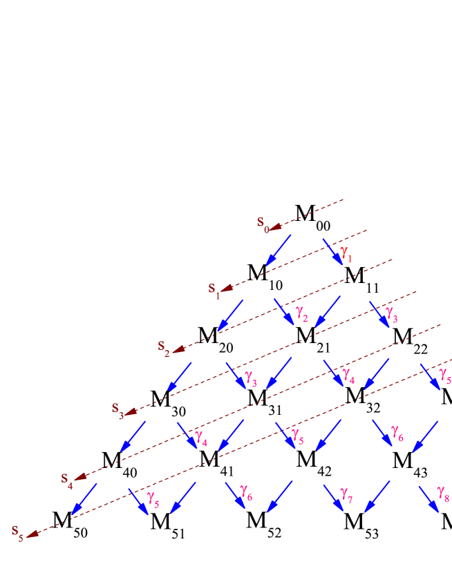
Figure 1: Solutions to the canonical three-term recurrence relation (34) from shallow unions in a generalized Pascal’s triangle.

From these sets we form the “shallow unions”

$$\mathcal{M}_{n}=\bigcup\limits_{k=0}^{\left\lfloor(n+1)/2\right\rfloor}M_{(n-k)k},$$ (39)

in analogy to the shallow sum in a standard Pascal’s triangle. Then the solution for the canonical three-term recurrence relation (34) can be expressed as

$$s_{n}=\sum\limits_{k=1}^{F_{n+1}}x_{k}\qquad\text{for }x_{k}\in\mathcal{M}_{n}\text{,}$$ (40)

where the number of elements in $\mathcal{M}_{n}$ equals the n-th Fibonacci number $F_{n}$, i.e. $F_{1}=1$, $F_{2}=1$, $F_{3}=2$, $F_{4}=3$, $F_{5}=5$, $F_{8}=8$,$\ldots$ The occurrence of the Fibonacci numbers is to be expected since for $\gamma_{n}=1$ the canonical relation (34) simply reduces to the well-known Fibonacci three-term recurrence relation and in this case (40) is just counting the elements in $\mathcal{M}_{n}$.

For the second Ansatz $\psi_{N}^{c}$ in (28) we may proceed in a similar fashion. Reading off the coefficients of $\cos(2n\theta)$ from the result of the substitution into the Schrödinger equation yields the same recursive equations (29) with $\sigma_{n}$ replaced by $c_{n}$

$$\zeta(2n-N-1)c_{n-1}+\left(4n^{2}+\zeta^{2}-E\right)c_{n}+\zeta(2n+1+N)c_{n+1}=0,$$ (41)

albeit only valid for $n=0,2,\ldots,(N-1)/2$. In addition we have the relation

$$\mathbf{2}\zeta(1-N)c_{0}+\left(4+\zeta^{2}-E\right)c_{1}+\zeta(3+N)c_{2}=0,$$ (42)

which is not part of the general family of equations (41) due to the factor 2 in the first term. Taking $c_{0}=1$ we solve (41) with $n=0$ for $c_{1}$, (42) for $c_{2}$, (41) with $n=2$ for $c_{3}$, until we reach the quantization condition at $n=(N-1)/2$. In this way we find

$$c_{1} = \frac{E-\zeta^{2}}{\zeta(N+1)},$$ (43)

$$c_{2} = \frac{E^{2}-2E\left(\zeta^{2}+2\right)}{\zeta^{2}(N+1)(N+3)}+\frac{\zeta^{2}+2N^{2}+2}{(N+1)(N+3)},$$ (44)

$$c_{3} = \frac{E^{3}-E^{2}\left(3\zeta^{2}+20\right)+E\left[3\zeta^{4}+\zeta^{2}\left(3N^{2}+29\right)+64\right]}{\zeta^{3}(N+1)(N+3)(N+5)}$$

$$-\frac{\zeta^{4}+9\zeta^{2}+\left(3\zeta^{2}+32\right)N^{2}+32}{\zeta(N+1)(N+3)(N+5)}.$$

Again these recurrence relations may be solved in closed form. We convert (41) and (42) into the canonical three-term relation form

$$q_{n+1}=q_{n}+\lambda_{n}q_{n-1},$$ (46)

by means of the substitutions

$$c_{n}=q_{n}\prod\limits_{k=0}^{n-1}\alpha_{k},\quad\lambda_{1}=\frac{2\beta_{1}}{\alpha_{1}\alpha_{0}},\quad\lambda_{\ell}=\frac{\beta_{\ell}}{\alpha_{\ell}\alpha_{\ell-1}},\quad\text{for }\ell\in\mathbb{N}_{0}\backslash\{1\}.$$ (47)

The functions $\alpha_{n}$ and $\beta_{n}$ are defined as in equation (35). Taking $q_{0}=1$, $q_{1}=1$, i.e. $c_{0}=q_{0}=1$, $c_{1}=q_{1}\alpha_{0}=\alpha_{0}$ the expression (36) yields a closed solution by replacing $\sigma_{n}\rightarrow c_{n}$ and $\gamma_{n}\rightarrow\lambda_{n}$, e.g. $c_{2}=q_{2}\alpha_{0}\alpha_{1}=(1+\lambda_{1})\alpha_{0}\alpha_{1}=\alpha_{0}\alpha_{1}+2\beta_{1}$, $c_{3}=q_{3}\alpha_{0}\alpha_{1}\alpha_{2}=(1+\lambda_{1}+\lambda_{2})\alpha_{0}\alpha_{1}\alpha_{2}=\alpha_{0}\alpha_{1}\alpha_{2}+2\beta_{1}\alpha_{2}+\beta_{2}\alpha_{0}$, etc.

3.2 Energy quantization and the double scaling limit

As mentioned, in the last step of the solution procedure for the recurrence relations we have no free coefficient function left. We can, however, fix the energy to a specific value, such that the last equation constitutes the energy quantization condition. We simple have to solve the algebraic expressions

$$\sigma_{(N+1)/2}=s_{(N-1)/2}\prod\limits_{k=1}^{(N-1)/2}\alpha_{k}=0\qquad\text{and\qquad}c_{(N+1)/2}=q_{(N+1)/2}\prod\limits_{k=0}^{(N-1)/2}\alpha_{k}=0,$$ (48)

for $E_{N}$ at specific values of $N$. We focus here on $N$ being odd as these are the interesting cases producing spectra that, depending on the values of $\zeta$, are real in part with fully unbroken $\mathcal{PT}$-symmetry and also possess spontaneously broken phases with energies occurring in complex conjugate pairs. For even values of $N$ the $\mathcal{PT}$-symmetry is broken throughout the entire range of $\zeta$. From (48) we observe that the degree of the polynomial in the energies $E_{N}$ equals the number of factors $\alpha_{k}$ in the product. Thus for the eigenfunctions related to the Ansatz (27) we find the corresponding energy eigenvalues $E_{N}^{s}$ from solving the first equation in (48), that is a $(N-1)/2$-th order equations in $E$, to

$$E_{3}^{s} = 4+\zeta^{2},$$ (49)

$$E_{5}^{s,\pm} = 10+\zeta^{2}\pm 2\sqrt{9-4\zeta^{2}},$$ (50)

$$E_{7}^{s,\ell} = \frac{56}{3}+\zeta^{2}+\frac{4}{3}e^{\frac{i\pi\ell}{3}}\Omega+\frac{4}{3}e^{-\frac{i\pi\ell}{3}}\Omega^{-1}\left(49-12\zeta^{2}\right),\qquad~{}~{}$$ (51)

with $\ell=0,\pm 2$ and $\Omega:=\left[143+72\zeta^{2}+6\sqrt{3}\sqrt{16\zeta^{6}-148\zeta^{4}+991\zeta^{2}-900}\right]^{1/3}$. For the solutions related to (28) we compute the eigenenergies $E_{N}^{s}$ by solving the first equation in (48), that is a $(N+1)/2$-th order equation in $E$, to

$$E_{1}^{c} = \zeta^{2},$$ (52)

$$E_{3}^{c,\pm} = 2+\zeta^{2}\pm 2\sqrt{1-4\zeta^{2}},$$ (53)

$$E_{5}^{c,\ell} = \frac{20}{3}+\zeta^{2}+\frac{4}{3}e^{\frac{i\pi\ell}{3}}\hat{\Omega}+\frac{4}{3}e^{-\frac{i\pi\ell}{3}}\hat{\Omega}^{-1}\left(13-12\zeta^{2}\right),\qquad~{}~{}$$ (54)

with $\ell=0,\pm 2$ and $\hat{\Omega}:=\left[35+72\zeta^{2}+6\sqrt{3}\sqrt{16\zeta^{6}-4\zeta^{4}+103\zeta^{2}-9}\right]^{1/3}$. At higher levels the expressions become increasingly complex and are therefore not reported here. However, using the generic solutions above they may be obtained easily in a numerical form, being just limited by computer power. As an example we depict the values for $N=9$ in figure 2.

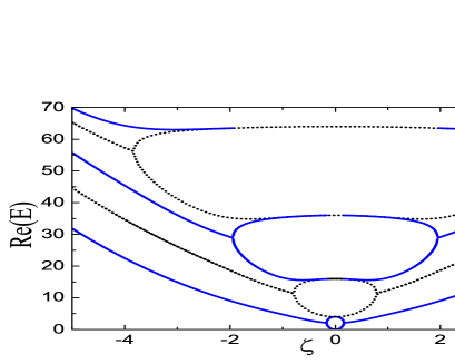
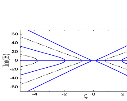
Figure 2: Energy eigenvalues $E_{9}$ as a function of $\zeta$ associated to odd (dotted, black) and even (solid, blue) eigenfunctions.

We observe the typical coalescence of two levels at the transition from the $\mathcal{PT}$-symmetric to the spontaneously broken regime marked by the so-called exceptional points [31, 32, 33, 34]. The precise values can be found by determining the real roots of the discriminants of the polynomials (48) in $E$ at the quantization level. Introducing the coefficients $a_{i}$ via the expansion for the polynomials by $P(E)=\sum\nolimits_{k=0}^{n}a_{k}E^{k}$, the discriminants can be computed easily from the determinants of the Sylvester matrix $S$ formed from $P(E)$ and its derivative $dP(E)/dE$ with entries

$$S_{ij}=\left\{\begin{array}[]{ll}a_{n+i-j},&\text{for }1\leq i\leq n-1,1\leq j\leq 2n-1,\\ (1+i-j)a_{1+i-j},&\text{for }n\leq i\leq 2n-1,1\leq j\leq 2n-1,\end{array}\right.$$ (55)

see for instance [35]. The discriminants are then given by $\det S=\kappa_{N}\Delta_{N}$. Dropping the overall factors $\kappa_{N}$ that do not contribute to the zeros we compute in this way

$$\Delta_{1}^{s} = \Delta_{1}^{c}=\Delta_{3}^{s}=1,$$ (56)

$$\Delta_{3}^{c} = 2^{2}\zeta^{2}-1,$$

$$\Delta_{5}^{s} = 2^{2}\zeta^{2}-9,$$

$$\Delta_{5}^{c} = 2^{4}\zeta^{6}-4\zeta^{4}+103\zeta^{2}-9,$$

$$\Delta_{7}^{s} = 2^{4}\zeta^{6}-148\zeta^{4}+991\zeta^{2}-900,$$

$$\Delta_{7}^{c} = 2^{8}\zeta^{12}+128\zeta^{10}+6160\zeta^{8}-132480\zeta^{6}+16128\zeta^{4}-183069\zeta^{2}+8100,$$

$$\Delta_{9}^{s} = 2^{8}\zeta^{12}-6016\zeta^{10}+112656\zeta^{8}-1526400\zeta^{6}+6645600\zeta^{4}-19579725\zeta^{2}+9922500~{}~{},~{}$$

$$\Delta_{9}^{c} = 2^{14}\zeta^{20}+40960\zeta^{18}+805888\zeta^{16}-50754048\zeta^{14}+1392155136\zeta^{12}+290722752\zeta^{10}$$

$$+11896163064\zeta^{8}-113625663975\zeta^{6}+8084618100\zeta^{4}-53543300400\zeta^{2}+1428840000,$$

$$\Delta_{11}^{s} = 2^{14}\zeta^{20}-778240\zeta^{18}+29068288\zeta^{16}-922894848\zeta^{14}+21572729856\zeta^{12}$$

$$-252561878208\zeta^{10}+2351098873944\zeta^{8}-15196772229975\zeta^{6}+39898457932725\zeta^{4}$$

$$-69457284086400\zeta^{2}+22684263840000$$

$$\Delta_{11}^{c} = 2^{22}\zeta^{30}+26214400\zeta^{28}+274464768\zeta^{26}-43646517248\zeta^{24}+2888883798016\zeta^{22}\ldots$$

The positive real roots $\zeta_{0}$ of these polynomials multiplied by $N$ are reported in table 1.

$N$	$\zeta_{0}N$	$\zeta_{0}N$	$\zeta_{0}N$	$\zeta_{0}N$	$\zeta_{0}N$
$3$	$1.50000$
$5$	$1.47963$	$7.50000$
$7$	$1.47426$	$7.19195$	$18.4246$
$9$	$1.47208$	$7.08219$	$17.5098$	$34.4001$
$11$	$1.47098$	$7.02966$	$17.1292$	$32.5974$	$55.4904$
	$\vdots$	$\vdots$	$\vdots$	$\vdots$	$\vdots$
$\infty$	$1.46877$	$6.92895$	$16.4711$	$30.0967$	$47.806$

Table 1: Values of $\zeta_{0}N$ computed from the positive real zeros $\zeta_{0}$ of the discriminant polynomials $\Delta_{N}(\zeta)$ converging to the critical values obtained from a Floquet method.

We observe that the product $\zeta_{0}N$ appears to converges to the critical values of the complex Mathieu equation energy eigenvalues related to the non-Hermitian Hamiltonian $\mathcal{H}_{\text{Mat}}^{\Pi^{(1)}}$ in (23), computed numerically using a Floquet method, i.e. imposing bosonic periodicity conditions $\psi(\theta+2\pi)=\psi(\theta)$. The smallest critical value at $N\rightarrow\infty$ is in agreement with the one reported in [36], whereas our values resulting from the smallest zero for $N=5,7$ differ slightly from those reported in [24]. Our values for $N\rightarrow\infty$ also agree precisely with those reported in [37] when divided by a factor 2. We observe, that the rate of convergence becomes very poor for larger values of the coupling constant and even the lowest value requires fairly large values of $N$ to reach a good precision.

A much better convergence can be obtained by taking the limit directly on the level of the three-term recurrence relation. We easily see that for $N\rightarrow\infty$, $\zeta\rightarrow 0$ with $g:=N\zeta<\infty$ and the assumption that the coefficient functions remain finite, i.e. $\lim_{N\rightarrow\infty,\zeta\rightarrow 0}\sigma_{n}=:\sigma_{n}^{M}$ and $\lim_{N\rightarrow\infty,\zeta\rightarrow 0}c_{n}=:c_{n}^{M}$, the relations (29), (41) and (42) reduce simply to

$$-g\sigma_{n-1}^{M}+4n^{2}\sigma_{n}^{M}+g\sigma_{n+1}^{M} = E\sigma_{n}^{M},$$ (57)

$$-gc_{n-1}^{M}+4n^{2}c_{n}^{M}+gc_{n+1}^{M} = Ec_{n}^{M},$$ (58)

$$-2gc_{0}^{M}+4c_{1}^{M}+g\sigma_{2}^{M} = Ec_{1}^{M}.$$ (59)

Rather than viewing these equations as recurrence relations we may also interpret them as two separate eigenvalue equations for the infinite matrices $\Xi$ and $\Theta$ with entries

$$\Xi_{i,j} = 4i^{2}\delta_{i,i}+g\delta_{i,i+1}-g\delta_{i+1,i},\quad\quad\qquad\qquad\quad\text{for }i,j\in\mathbb{N},$$ (60)

$$\Theta_{i,j} = 4i^{2}\delta_{i,i}+g\delta_{i,i+1}-g\delta_{i+1,i}-g\delta_{i,2}\delta_{j,1},\quad\quad\text{for }i,j\in\mathbb{N}_{0},$$ (61)

acting on the vectors $(\sigma_{1}^{M},\sigma_{2}^{M},\sigma_{3}^{M},\ldots)$ and $(c_{0}^{M},c_{1}^{M},\sigma_{1}^{M},\ldots)$, respectively. Truncating the matrices at a certain level, say $\ell$, we compute the characteristic polynomials $\det(\Xi^{\ell}-E\mathbb{I})$ and $\det(\Theta^{\ell}-E\mathbb{I})$ together with their corresponding discriminants $\Delta^{\Xi}(g)$ and $\Delta^{\Theta}(g)$ from (55). The real zeros $g_{0}$ of these $\ell(\ell-1)$-order polynomials define the exceptional points. We present our numerical results in tables 2 and 3.

$\ell$	$g_{0}$	$g_{0}$	$g_{0}$	$g_{0}$	$g_{0}$	$g_{0}$	$g_{0}$
$2$	$6.00000$
$3$	$6.97891$
$4$	$6.92848$	$18.77091$
$5$	$6.92896$	$24.29547$
$6$	$6.92895$	$29.26843$	$29.73862$
$7$	$6.92895$	$30.10798$	$34.30404$
$8$	$6.92895$	$30.09660$	$39.34849$	$61.30789$
$\vdots$	$\vdots$	$\vdots$	$\vdots$	$\vdots$
$26$	$6.928955$	$30.09677$	$69.59879$	$125.4354$	$130.5181$	$197.6067$	$251.2637$
$27$	$\mathbf{6.928955}$	$\mathbf{30.09677}$	$\mathbf{69.59879}$	$\mathbf{125.4354}$	$135.5878$	$\mathbf{197.6067}$	$261.6061$
$26$	$286.1126$	$357.0076$	$390.9532$	$448.0887$	$511.0770$	$525.2021$
$27$	$\mathbf{286.1126}$	$372.5999$	$\mathbf{390.9532}$	$468.8640$	$512.1858$	$551.0671$

Table 2: Real zeros $g_{0}$ of the discriminant polynomials $\Delta^{\Xi}(g)$ converging to the exceptional points marked in bold.

$\ell$	$g_{0}$	$g_{0}$	$g_{0}$	$g_{0}$	$g_{0}$	$g_{0}$	$g_{0}$
$2$	$1.41421$
$3$	$1.46904$
$4$	$1.46877$	$12.34951$
$5$	$1.46877$	$17.88618$
$6$	$1.46877$	$16.44658$	$24.21371$
$7$	$1.46877$	$16.47150$	$29.27154$
$8$	$1.46877$	$16.47116$	$34.30396$	$45.47616$
$\vdots$	$\vdots$	$\vdots$	$\vdots$	$\vdots$
$26$	$1.46877$	$16.47117$	$47.80597$	$95.47527$	$125.4485$	$159.4792$	$239.8178$
$27$	$\mathbf{1.46877}$	$\mathbf{16.47117}$	$\mathbf{47.80597}$	$\mathbf{95.47527}$	$130.5181$	$\mathbf{159.4792}$	$\mathbf{239.8178}$
$26$	$240.9227$	$336.4911$	$341.4216$	$427.3330$	$449.3487$	$498.9970$
$27$	$251.2637$	$\mathbf{336.4911}$	$357.0076$	$448.0887$	$449.5057$	$525.2659$

Table 3: Real zeros $g_{0}$ of the discriminant polynomials $\Delta^{\Theta}(g)$ converging to the exceptional points marked in bold.

As a simple criterion we take the stabilization to a fixed value at some given precision for two consecutive truncation levels. Taking for instance the truncation levels to be $26$ and $27$ we have identified 14 exceptional points marked in bold in our tables. All known values obtained agree with those reported in the literature. Already at this level we find several new values and it would be easy to extend these computation to higher truncation levels being simply limited by computer power. Evidently solving the characteristic polynomials for the energies and eigenvectors will provide a good solution for the complete eigenvalue problem of $\mathcal{H}_{\text{Mat}}^{\Pi^{(1)}}$, i.e. the eigenvectors and eigenfunctions, which we will however not present here.

In a loose sense the discrete eigenvalue problem considered here is somewhat similar in spirit to Znojil’s [38, 39, 40] discretized versions for non-Hermitian systems, although the discrete nature of the problem results here from the coefficients in the expansion of the eigenfunction rather than from the space on which they are defined. In a slightly different approach the first levels of discretized version of the complex Mathieu equation for some even solutions were also recently reported in [41].

3.3 Factorization beyond the quantization level

In our Ansatz we have truncated the Fourier series at a specific value, which led to the quantization condition (48). In fact this is not necessary and instead we may also consistently consider the infinite series $\psi_{N\rightarrow\infty}^{s}(\theta)$ and $\psi_{N\rightarrow\infty}^{c}(\theta)$ with $\zeta$ finite, i.e. here this is not to be understood as a double scaling limit. Imposing then the quantization condition by hand at some level all higher terms in the series above will automatically vanish. This effect results from the factorization property of the polynomials beyond that level in a similar fashion well known for the Bender-Dunne polynomials [26]. We find here

$$\sigma_{M+n}=\sigma_{M+1}Q_{n-1},\qquad\text{and\qquad}c_{L+m}=c_{L}Q_{m}\qquad\text{for }n\in\mathbb{N},m\in\mathbb{N}_{0},$$ (62)

where we denoted $M=(N-1)/2$ and $L=(N+1)/2$. We will now provide expressions for the polynomials $Q_{n}$. The factorization is easily understood by noting first that $\gamma_{M}=0$, which simply has the effect to reset the recurrence relations to the beginning, albeit with different initial conditions. By inspection we see that the recurrence relations (34) from the level $M$ onwards simply reduces to $s_{M+1}=s_{M}$, $s_{M+2}=(1+\gamma_{M+1})s_{M}$, $s_{M+3}=(1+\gamma_{M+1}+\gamma_{M+2})s_{M}$, $s_{M+4}=(1+\gamma_{M+1}+\gamma_{M+2}+\gamma_{M+3}+\gamma_{M+1}\gamma_{M+3})s_{M}$, etc. Thus apart from the overall factor of $s_{M}$, we simply recover the original solutions for $s_{n}$ with all functions $\gamma_{i}$ replaced by $\gamma_{i+M}$. Therefore we obtain the solutions

$$s_{M+n}=s_{n}(\gamma_{i}\rightarrow\gamma_{i+M})s_{M}\qquad\text{for }n\in\mathbb{N}_{0}.$$ (63)

Using the first relation in (48) this becomes

$$\sigma_{M+n}=\sigma_{M+1}s_{n-1}(\gamma_{i}\rightarrow\gamma_{i+M})\prod\limits_{k=M+1}^{M+n-1}\alpha_{k}=\sigma_{M+1}\hat{\sigma}_{n},$$ (64)

from which we may read of the polynomials $\hat{\sigma}_{n}$. For instance, we have

$$\hat{\sigma}_{1} = 1,$$ (65)

$$\hat{\sigma}_{2} = \alpha_{M+1},$$ (66)

$$\hat{\sigma}_{3} = \alpha_{M+1}\alpha_{M+2}+\beta_{M+2},$$ (67)

$$\hat{\sigma}_{4} = \alpha_{M+1}\alpha_{M+2}\alpha_{M+3}+\beta_{M+2}\alpha_{M+3}+\beta_{M+3}\alpha_{M+1}.$$ (68)

Likewise noting that $\lambda_{L}=0$, the recurrence relations (46) from that level onwards become $q_{L+1}=q_{L}$, $q_{L+2}=(1+\lambda_{L+1})q_{L}$, etc. and therefore

$$q_{L+n}=q_{n}(\lambda_{i}\rightarrow\lambda_{i+L})q_{L}\qquad\text{for }n\in\mathbb{N}_{0}.$$ (69)

The first relation in (47) then yields

$$c_{L+n}=c_{L}q_{n}(\lambda_{i}\rightarrow\lambda_{i+L})\prod\limits_{k=L}^{L+n-1}\alpha_{k}=c_{L}\hat{c}_{n},$$ (70)

from which we may identify the polynomials $\hat{c}_{n}$. We obtain for example $\hat{c}_{0}=1$, $\hat{c}_{1}=\alpha_{L}$, $\hat{c}_{2}=\alpha_{L}\alpha_{L+1}+\beta_{L+1}$, etc. We observe that $\hat{c}_{i}=\hat{\sigma}_{i+1}=Q_{i}$ for $i=0,1,2,\ldots$, thus establishing (62).

3.4 Weakly orthogonal polynomials

As seen in the previous subsection our univariate polynomials $\sigma_{n}(E)$ and $c_{n}(E)$ enjoy similar properties as the Bender-Dunne polynomials and are therefore expected to be also weakly orthogonal polynomials in $E$ in the sense defined in [28, 42]. We briefly recall the formalism and details of how this is achieved. As pointed out in [28], according to Favard’s theorem [27] on three-term recurrence relations of the general form

$$\Phi_{n+1}=\left(E-a_{n}\right)\Phi_{n}-b_{n}\Phi_{n-1},$$ (71)

with $b_{n}=0$ for $n\leq 0$ and $b_{K}=0$, there exists always a linear functional $\mathcal{L}$ acting on arbitrary polynomials $p$ as

$$\mathcal{L}(p)=\int\nolimits_{-\infty}^{\infty}p(E)\omega(E)dE,$$ (72)

such that the polynomials $\Phi_{n}(E)$ are orthogonal

$$\mathcal{L}(\Phi_{n}\Phi_{m})=\mathcal{L}(E\Phi_{n}\Phi_{m-1})=N_{n}\delta_{nm}.$$ (73)

Thus the constants $N_{n}$ constitute the squared norms of $\Phi_{n}$. The second equation in (73) is a simple consequence of the first and (71). The functional is unique [28] with the specific initial conditions $\mathcal{L}(\Phi_{0}=1)=1$. The measure $\omega(E)$ is given by the equations

$$\omega(E)=\sum\limits_{k=1}^{K}\omega_{k}\delta(E-E_{k}),$$ (74)

where the energies $E_{k}$ are the $K$ roots of the polynomial $\Phi_{K}$ and the $K$ constants $\omega_{k}$ are determined by the $K$ equations

$$\sum\limits_{k=1}^{K}\omega_{k}\Phi_{n}(E_{k})=\delta_{n0}\text{,}\qquad\text{for }n\in\mathbb{N}_{0}.$$ (75)

The squared norms $N_{n}$ may also be computed in an alternative way. Multiplying (71) by $\Phi_{n-1}$ and subsequently acting on it with $\mathcal{L}$, assuming that it exists and satisfies (73), we obtain the simple homogeneous two-term relation

$$N_{n}=b_{n}N_{n-1},\qquad\text{for }n\in\mathbb{N}.$$ (76)

Using the initial condition $N_{0}=1$ this is easily solved to

$$N_{n}=\left\{\begin{array}[]{ll}\prod\limits_{k=1}^{n}b_{k},&\text{for }1\leq n<K,\\ 0,&\text{for }n\geq K.\end{array}\right.$$ (77)

Thus as already pointed out in [26] we may compute the squared norms without the knowledge of the measure.

A further quantity which is easily computed with the knowledge of the explicit form of $\mathcal{L}$ are the moment functionals as pointed out in [27, 28]. They are defined as

$$\mu_{n}:=\mathcal{L}(E^{n})=\sum\limits_{k=1}^{K}\int\nolimits_{-\infty}^{\infty}E^{n}\omega_{k}\delta(E-E_{k})dE=\sum\limits_{k=1}^{K}\omega_{k}E_{k}^{n},$$ (78)

Once again also these quantities can be obtained alternatively from the original polynomials without the knowledge of the $\omega_{k}$. Defining the coefficients $\nu_{k}^{(n)}$ by the relation $\Phi_{n}(E)=E^{n}-\sum\nolimits_{k=0}^{n-1}\nu_{k}^{(n)}E^{k}$ and acting on this equation with $\mathcal{L}$ we obtain

$$\mu_{n}=\sum\limits_{k=0}^{n-1}\nu_{k}^{(n)}\mu_{k}.$$ (79)

Evidently this allows for a recursive construction of all constants $\mu_{n}$ when all polynomials $\Phi_{k}(E)$ with $k\leq n$ are known.

As a consistency check on the wavefunctions one may also compute

$$\mathcal{L}\left[\psi(\theta,E)\right]=\sum\limits_{k=1}^{K}\int\nolimits_{-\infty}^{\infty}\psi(\theta,E)\omega_{k}\delta(E-E_{k})dE=\sum\limits_{k=1}^{K}\omega_{k}\psi(\theta,E_{k}).$$ (80)

As a consequence of (75) we expect for our wave functions (27) and (28) the simple expressions

$$\mathcal{L}\left[\psi_{N}^{s}(\theta,E)\right]=-\sin(2\theta)e^{\frac{i}{2}\zeta\cos(2\theta)},\quad\text{and\quad}\mathcal{L}\left[\psi_{N}^{c}(\theta,E)\right]=e^{\frac{i}{2}\zeta\cos(2\theta)}.$$ (81)

Let us now apply the above further to our system. For this purpose we extract from the $\sigma_{n}(E)$ the denominator by introducing the new polynomials $P_{n}(E)$ via the relation $\sigma_{n}=P_{n-1}\zeta^{1-n}\prod\nolimits_{k=1}^{n-1}(N+1+2k)^{-1}$. The three-term recurrence equation (29) then translates into a relation for the polynomials $P_{n}$

$$P_{n+1}=\left[E-\zeta^{2}-4(n+1)^{2}\right]P_{n}+\zeta^{2}\left[N^{2}-(1+2n)^{2}\right]P_{n-1},\quad n\in\mathbb{N}_{0}.$$ (82)

Comparing with the generic form (71) we identify $\Phi_{n}=P_{n}$ and the constants $a_{n}=$ $\zeta^{2}+4(n+1)^{2}$, $b_{n}=\zeta^{2}\left[(1+2n)^{2}-N^{2}\right]$. Since $b_{M}=0$ our critical cut off level is $K=M$. Therefore the squared norms result from (77) to

$$N_{n}=\left\{\begin{array}[]{ll}4^{n}\zeta^{2n}\left(\frac{3}{2}-\frac{N}{2}\right)_{n}\left(\frac{3}{2}+\frac{N}{2}\right)_{n},&\text{for }1\leq n\leq(N-3)/2,\\ 0,&\text{for }n>(N-3)/2,\end{array}\right.$$ (83)

where $(a)_{n}:=\Gamma\left(a+n\right)/\Gamma\left(a\right)$ denotes the Pochhammer symbol.

For concrete values of $N$ these expressions are easily computed. Taking for instance $N=7$ our general expressions for $\sigma_{n}$ yield

$$P_{0}(E) = 1,$$ (84)

$$P_{1}(E) = E-\zeta^{2}-4,$$

$$P_{2}(E) = E^{2}-2E\left(\zeta^{2}+10\right)+\zeta^{4}+60\zeta^{2}+64,$$

$$P_{3}(E) = E^{3}-E^{2}\left(3\zeta^{2}+56\right)+E\left(3\zeta^{4}+176\zeta^{2}+784\right)-\zeta^{6}-120\zeta^{4}-2320\zeta^{2}-2304,$$

$$P_{4}(E) = \left(E-\zeta^{2}-64\right)P_{3}(E),$$

$$P_{5}(E) = \left[E^{2}-2E\left(\zeta^{2}+82\right)+\zeta^{4}+132\zeta^{2}+6400\right]P_{3}(E).$$

We observe the typical factorization above the quantization level, that is $M=3$ in this case. The roots of the polynomial $P_{3}(E)$ were computed before in (51). Assigning here $E_{1}:=E_{7}^{s,-2}$, $E_{2}:=E_{7}^{s,2}$ and $E_{3}:=E_{7}^{s,0}$ we solve the three equations (75) for the constants $\omega_{k}$. We find

$$\omega_{1}=\varkappa_{2},\qquad\omega_{2}=\varkappa_{-2},\qquad\omega_{3}=\varkappa_{0}.$$ (85)

where we abbreviated

$$\varkappa_{\ell}:=\frac{2\left(49-12\zeta^{2}\right)^{2}+3\left(48-7\zeta^{2}\right)e^{-\frac{i\pi\ell}{3}}\Omega^{2}+22\left(12\zeta^{2}-49\right)e^{\frac{i\pi\ell}{3}}\Omega+2e^{\frac{i\pi\ell}{3}}\Omega^{4}-22\Omega^{3}}{6\left[\left(49-12\zeta^{2}\right)^{2}+\left(49-12\zeta^{2}\right)e^{-\frac{i\pi\ell}{3}}\Omega^{2}+e^{\frac{i\pi\ell}{3}}\Omega^{4}\right]},$$

with $\Omega$ as defined after (51). This gives a complicated measure, but when computing the integrals the result simplifies to

$$\mathcal{L}(P_{0}^{2}) = \omega_{1}+\omega_{2}+\omega_{3}=1=N_{0},$$ (86)

$$\mathcal{L}(P_{1}^{2}) = \omega_{1}P_{1}^{2}(E_{1})+\omega_{2}P_{1}^{2}(E_{2})+\omega_{3}P_{1}^{2}(E_{3})=-40\zeta^{2}=N_{1},$$ (87)

$$\mathcal{L}(P_{2}^{2}) = \omega_{1}P_{2}^{2}(E_{1})+\omega_{2}P_{2}^{2}(E_{2})+\omega_{3}P_{2}^{2}(E_{3})=960\zeta^{4}=N_{2},$$ (88)

$$\mathcal{L}(P_{m}^{2}) = 0,\qquad\text{for }m\geq 3,$$ (89)

$$\mathcal{L}(P_{n}P_{m}) = 0,\qquad\text{for }m\neq n\text{; }n,m\in\mathbb{N}_{0}.$$ (90)

where (86) - (88) agree exactly with the expressions computed from (83). In (90) especially $\mathcal{L}(P_{1}P_{2})$ is a non-trivial check. We also recover the first expression in (81) when using (85).

Employing next the formula (78) together with (85) we compute the first momentum functionals to

$$\mu_{0} = 1,$$ (91)

$$\mu_{1} = \zeta^{2}+4,$$ (92)

$$\mu_{2} = \zeta^{4}-32\zeta^{2}+16,$$ (93)

$$\mu_{3} = \zeta^{6}-108\zeta^{4}-912\zeta^{2}+64,$$ (94)

$$\mu_{4} = \zeta^{8}-224\zeta^{6}-1184\zeta^{4}-17024\zeta^{2}+256.$$ (95)

We easily verify that these expressions also satisfy the relation (79) together with (84).

Turning now to our second set of recurrence relations (41), (42) we proceed in a similar fashion and extract the denominator $c_{n}(E)$ by introducing the new polynomials $\hat{P}_{n}(E)$ via $c_{n}=\hat{P}_{n}\zeta^{-n}\prod\nolimits_{k=1}^{n}(N+2k-1)^{-1}$. The three-term recurrence relations (41), (42) then becomes

$$\hat{P}_{n+1} = \left(E-\zeta^{2}-4n^{2}\right)\hat{P}_{n}+\zeta^{2}\left[N^{2}-(2n-1)^{2}\right]\hat{P}_{n-1},\quad n\in\mathbb{N}_{0}\backslash\{1\},$$ (96)

$$\hat{P}_{2} = \left(E-\zeta^{2}-4\right)\hat{P}_{1}+2\zeta^{2}\left(N^{2}-1\right)\hat{P}_{0}.$$ (97)

Now we identify $\Phi_{n}=\hat{P}_{n}$ and the constants $\hat{a}_{n}=$ $\zeta^{2}+4n^{2}$ for $n\in\mathbb{N}_{0}$, $\hat{b}_{1}=$ $2\zeta^{2}\left(N^{2}-1\right),\hat{b}_{n}=\zeta^{2}\left[(2n-1)^{2}-N^{2}\right]$ for $n\in\mathbb{N}_{0}\backslash\{1\}$. Since $b_{L}=0$ our critical cut off level results to $K=L$. The squared norms computed from (77) are

$$\hat{N}_{n}=\left\{\begin{array}[]{ll}2^{2n+1}\zeta^{2n}\left(\frac{1}{2}-\frac{N}{2}\right)_{n}\left(\frac{1}{2}+\frac{N}{2}\right)_{n},&\text{for }1\leq n\leq(N-1)/2,\\ 0,&\text{for }n>(N-1)/2.\end{array}\right.$$ (98)

As an example we take now $N=5$ in our general expressions for $c_{n}$ obtaining

$$\hat{P}_{0}(E) = 1,$$ (99)

$$\hat{P}_{1}(E) = E-\zeta^{2},$$

$$\hat{P}_{2}(E) = E^{2}-2E\left(\zeta^{2}+2\right)+\zeta^{2}\left(\zeta^{2}+52\right),$$

$$\hat{P}_{3}(E) = E^{3}+E^{2}\left(-3\zeta^{2}-20\right)+E\left(3\zeta^{4}+104\zeta^{2}+64\right)-\zeta^{2}\left(\zeta^{4}+84\zeta^{2}+832\right)$$

$$\hat{P}_{4}(E) = \left(E-\zeta^{2}-36\right)\hat{P}_{3}(E),$$

$$\hat{P}_{5}(E) = \left[E^{2}-2E\left(\zeta^{2}+50\right)+\zeta^{4}+76\zeta^{2}+2304\right]\hat{P}_{3}(E).$$

As expected the polynomials factorize again after the quantization level. Assigning now the previously computed roots of $\hat{P}_{3}(E)$, see (54), as $E_{1}=E_{5}^{c,-2}$, $E_{2}=E_{5}^{c,2}$ and $E_{3}=E_{5}^{c,0}$ we solve the three equations (75) for the constants $\omega_{k}$. We compute

$$\hat{\omega}_{1}=\hat{\varkappa}_{2},\qquad\hat{\omega}_{2}=\hat{\varkappa}_{-2},\qquad\hat{\omega}_{3}=\hat{\varkappa}_{0}.$$ (100)

where we defined the function

$$\hat{\varkappa}_{\ell}:=\frac{\left(13-12\zeta^{2}\right)^{2}+\left(12-15\zeta^{2}\right)e^{-\frac{i\pi k}{3}}\hat{\Omega}^{2}+\left(60\zeta^{2}-65\right)e^{\frac{i\pi k}{3}}\hat{\Omega}+e^{\frac{i\pi k}{3}}\hat{\Omega}^{4}-5\hat{\Omega}^{3}}{3\left(13-12\zeta^{2}\right)^{2}+\left(39-36\zeta^{2}\right)e^{-\frac{i\pi k}{3}}\hat{\Omega}^{2}+3e^{\frac{i\pi k}{3}}\hat{\Omega}^{4}},$$

with $\hat{\Omega}$ as introduced after (54). Next we use this measure to evaluate

$$\mathcal{L}(\hat{P}_{0}^{2}) = \hat{\omega}_{1}+\hat{\omega}_{2}+\hat{\omega}_{3}=1=\hat{N}_{0},$$ (101)

$$\mathcal{L}(\hat{P}_{1}^{2}) = \hat{\omega}_{1}P_{1}^{2}(E_{1})+\hat{\omega}_{2}P_{1}^{2}(E_{2})+\hat{\omega}_{3}P_{1}^{2}(E_{3})=-48\zeta^{2}=\hat{N}_{1},$$ (102)

$$\mathcal{L}(\hat{P}_{2}^{2}) = \hat{\omega}_{1}P_{2}^{2}(E_{1})+\hat{\omega}_{2}P_{2}^{2}(E_{2})+\hat{\omega}_{3}P_{2}^{2}(E_{3})=768\zeta^{4}=\hat{N}_{2},$$ (103)

$$\mathcal{L}(\hat{P}_{m}^{2}) = 0,\qquad\text{for }m\geq 3,$$ (104)

$$\mathcal{L}(\hat{P}_{n}\hat{P}_{m}) = 0,\qquad\text{for }m\neq n\text{; }n,m\in\mathbb{N}_{0}.$$ (105)

We verify that the results for $\hat{N}_{1}$ and $\hat{N}_{2}$ obtained by direct integration agree precisely with those computed from the expression in (98). In addition, we recover the second identity in (81) from the integration with (100).

Using formula (78) together with (100) we compute the first momentum functionals to

$$\hat{\mu}_{0} = 1,$$ (106)

$$\hat{\mu}_{1} = \zeta^{2},$$ (107)

$$\hat{\mu}_{2} = \zeta^{4}-48\zeta^{2},$$ (108)

$$\hat{\mu}_{3} = \zeta^{6}-144\zeta^{4}-192\zeta^{2},$$ (109)

$$\hat{\mu}_{4} = \zeta^{8}-288\zeta^{6}+2304\zeta^{4}-768\zeta^{2},$$ (110)

which again agree with those evaluated from (79).

4 Conclusions and outlook

We have demonstrated that $E_{2}$-quasi-exact solvability allows for a systematic construction of solutions to the eigenvalue problem for models that can be cast into that form. For the non-Hermitian models presented here, $\mathcal{H}_{N}$, but especially $\mathcal{H}_{\text{Mat}}$, the analysis seems to be more natural, easier and transparent than in a $sl_{2}(\mathbb{C})$-setting. A sharper comparison between the two schemes can of course be developed. Obviously the above analysis is not restricted to non-Hermitian systems, which were selected as they are of current interest, especially in the context of optics [16, 17, 18, 19, 20, 21, 22]. There is large scope to search for other models that are $E_{2}$-quasi-exactly solvable by modifying the vector spaces (5) and (6) by adjusting them for Hermitian models or systems possessing different types of $\mathcal{PT}$-symmetry as identified in [15].

In the analysis of the complex Mathieu equation we have mainly focused here on the identification of the exceptional points. In that regard we demonstrated that the double scaling limit for $\mathcal{H}_{N}$ level by level provides a very good qualitative picture for the Mathieu system, but to achieve quantitative precision requires to compute very high levels. Alternatively it is much easier and efficient to carry out the limit directly for the three-term recurrence relation and view that equation as an eigenvalue equation. One is still left with an entirely algebraic setting and convergence is achieved very fast. We have reported several hitherto unknown exceptional points. The latter approach is also far more efficient than the Floquet method, which for the problem discussed becomes very unstable for large values of $\zeta$ .

References

• [1] F. Calogero, Solution of a three-body problem in one-dimension, J. Math. Phys. 10, 2191–2196 (1969).
• [2] A. Fring and C. Korff, Exactly solvable potentials of Calogero type for q-deformed Coxeter groups, J. Phys. A37, 10931–10950 (2004).
• [3] B. Sutherland, Exact results for a quantum many body problem in one- dimension, Phys. Rev. A4, 2019–2021 (1971).
• [4] M. A. Olshanetsky and A. M. Perelomov, Classical integrable finite dimensional systems related to Lie algebras, Phys. Rept. 71, 313–400 (1981).
• [5] M. A. Olshanetsky and A. M. Perelomov, Quantum integrable systems related to Lie algebras, Phys. Rept. 94, 313–404 (1983).
• [6] A. V. Turbiner, Quasi-Exactly-Solvable problems and sl(2) Algebra, Commun. Math. Phys. 118, 467–474 (1988).
• [7] A. Turbiner, Lie algebras and linear operators with invariant subspaces, Lie Algebras, Cohomologies and New Findings in Quantum Mechanics, Contemp. Math. AMS, (eds N. Kamran and P.J. Olver) 160, 263–310 (1994).
• [8] J. E. Humphreys, Introduction to Lie Algebras and Representation Theory, Springer, Berlin (1972).
• [9] P. E. G. Assis and A. Fring, Non-Hermitian Hamiltonians of Lie algebraic type, J. Phys. A42, 015203 (23p) (2009).
• [10] P. E. G. Assis, Metric operators for non-Hermitian quadratic su(2) Hamiltonians, J. Phys. A44, 265303 (2011).
• [11] F. G. Scholtz, H. B. Geyer, and F. Hahne, Quasi-Hermitian Operators in Quantum Mechanics and the Variational Principle, Ann. Phys. 213, 74–101 (1992).
• [12] C. M. Bender and S. Boettcher, Real Spectra in Non-Hermitian Hamiltonians Having PT Symmetry, Phys. Rev. Lett. 80, 5243–5246 (1998).
• [13] C. M. Bender, Making sense of non-Hermitian Hamiltonians, Rept. Prog. Phys. 70, 947–1018 (2007).
• [14] A. Mostafazadeh, Pseudo-Hermitian Representation of Quantum Mechanics, Int. J. Geom. Meth. Mod. Phys. 7, 1191–1306 (2010).
• [15] S. Dey, A. Fring, and T. Mathanaranjan, Non-Hermitian systems of Euclidean Lie algebraic type with real eigenvalue spectra, Annals of Physics 346, 28–41 (2014).
• [16] Z. H. Musslimani, K. G. Makris, R. El-Ganainy, and D. N. Christodoulides, Optical Solitons in PT Periodic Potentials, Phys. Rev. Lett. 100, 030402 (2008).
• [17] K. G. Makris, R. El-Ganainy, D. N. Christodoulides, and Z. H. Musslimani, PT-symmetric optical lattices, Phys. Rev. A81, 063807(10) (2010).
• [18] A. Guo, G. J. Salamo, D. Duchesne, R. Morandotti, M. Volatier-Ravat, V. Aimez, G. A. Siviloglou, and D. Christodoulides, Observation of PT-Symmetry Breaking in Complex Optical Potentials, Phys. Rev. Lett. 103, 093902(4) (2009).
• [19] B. Midya, B. Roy, and R. Roychoudhury, A note on the PT invariant potential $4cos^{2}x+4iV_{0}sin2x$, Phys. Lett. A374, 2605 – 2607 (2010).
• [20] H. Jones, Use of equivalent Hermitian Hamiltonian for PT-symmetric sinusoidal optical lattices, J. Phys. A44, 345302 (2011).
• [21] E. Graefe and H. Jones, PT-symmetric sinusoidal optical lattices at the symmetry-breaking threshold, Phys. Rev. A84, 013818(8) (2011).
• [22] S. Longhi and G. Della Valle, Invisible defects in complex crystals, Annals of Physics 334, 35–46 (2013).
• [23] A. Khare and B. P. Mandal, A PT-invariant potential with complex QES eigenvalues, Phys. Lett. A 272, 53–56 (2000).
• [24] B. Bagchi, S. Mallik, C. Quesne, and R. Roychoudhury, A PT-symmetric QES partner to the Khare–Mandal potential with real eigenvalues, Phys. Lett. A 289, 34–38 (2001).
• [25] B. Bagchi, C. Quesne, and R. Roychoudhury, A complex periodic QES potential and exceptional points, J. Phys. A 41, 022001 (2008).
• [26] C. M. Bender and G. V. Dunne, Quasiexactly solvable systems and orthogonal polynomials, J. Math. Phys. 37, 6–11 (1996).
• [27] J. Favard, Sur les polynomes de Tchebicheff., C. R. Acad. Sci., Paris 200, 2052–2053 (1935).
• [28] F. Finkel, A. Gonzalez-Lopez, and M. A. Rodriguez, Quasiexactly solvable potentials on the line and orthogonal polynomials, J. Math. Phys. 37, 3954–3972 (1996).
• [29] C. J. Isham and N. Linden, Group theoretic quantisation of strings on tori, Classical and Quantum Gravity 5, 71–93 (1988).
• [30] I. Gonoskov, Closed-form solution of a general three-term recurrence relation, Advances in Difference Equations 2014, 196(12) (2014).
• [31] T. Kato, Perturbation Theory for Linear Operators, (Springer, Berlin) (1966).
• [32] W. D. Heiss, Repulsion of resonance states and exceptional points, Phys. Rev. E 61, 929–932 (2000).
• [33] I. Rotter, Exceptional points and double poles of the $S$ matrix, Phys. Rev. E 67, 026204 (2003).
• [34] U. Günther, I. Rotter, and B. F. Samsonov, Projective Hilbert space structures at exceptional points, J. Phys. A40(30), 8815 (2007).
• [35] A. G. Akritas, Sylvester’s forgotten form of the resultant, Fibonacci Quart , 325–332 (1993).
• [36] H. P. Mulholland and S. Goldstein, The characteristic numbers of the Mathieu equation with purely imaginary parameter, The London, Edinburgh, and Dublin Philosophical Magazine and Journal of Science 8, 834–840 (1929).
• [37] C. M. Bender and R. J. Kalveks, Extending PT Symmetry from Heisenberg Algebra to E2 Algebra, Int. J. of Theor. Phys. 50, 955–962 (2011).
• [38] M. Znojil, One-dimensional Schrödinger equation and its exact representation on a discrete lattice, Phys. Lett. 223, 411–416 (1996).
• [39] M. Znojil, Discrete quantum square well of the first kind, Phys. Lett. 375, 2503–2509 (2011).
• [40] M. Znojil, Solvable non-Hermitian discrete square well with closed-form physical inner product, J. Phys. A: Math. Theor. 47, 435302 (2014).
• [41] C. H. Ziener, M. Rückl, T. Kampf, W. R. Bauer, and H. P. Schlemmer, Mathieu functions for purely imaginary parameters, Journal of Computational and Applied Mathematics 236, 4513––4524 (2012).
• [42] A. Krajewska, A. Ushveridze, and Z. Walcza, Bender–Dunne Orthogonal Polynomials General Theory, Mod. Phys. Lett. A 12, 1131–1144 (1997).