Analytic Structure of the S-Matrix
for Singular Quantum Mechanics

Abstract

The analytic structure of the S-matrix of singular quantum mechanics is examined within a multichannel framework, with primary focus on its dependence with respect to a parameter ($\Omega$) that determines the boundary conditions. Specifically, a characterization is given in terms of salient mathematical and physical properties governing its behavior. These properties involve unitarity and associated current-conserving Wronskian relations, time-reversal invariance, and Blaschke factorization. The approach leads to an interpretation of effective nonunitary solutions in singular quantum mechanics and their determination from the unitary family.

I Introduction

Singular potentials are known to pose notoriously subtle difficulties that call for an extension of the rules of ordinary quantum mechanics. Some of the outstanding problematic features of singular quantum mechanics (SQM) were addressed in the pioneering work of Ref. cas:50 and in the early literature reviewed in Refs. spector_RMP and Newton . These features can be ultimately traced to an indeterminacy in the boundary conditions landau:77 . More recent general frameworks were proposed in Ref. Esposito using polydromy properties Stroffolini , and in Ref. Smatrix-singularQM within a general multichannel framework. In addition, significant progress has been made for specific problems related to the renormalization of the inverse square potential (ISP) Gupta-1993 ; HEC-LP1 ; HEC-LP2 ; HEC:CQM-renormalization and contact interactions Jackiw-1991-Beg , their associated conformal symmetry Alfaro-Fubini-Furlan-1976 ; Jackiw_SO(21)_1 ; Jackiw_SO(21)_2 and anomaly HEC-CQManomaly1 ; HEC-CQManomaly2 , and other cases of SQM renormalization Beane:2000wh .

In this paper, we reexamine the generic form of the S-matrix for SQM and shed light on the existence of an intriguing connection between the unitary and nonunitary solutions. A particular form of this connection can be found in the pioneering work of Ref. radin:75 , where it was pointed out that, while the basic results of Ref. cas:50 focus on the unitary but nonunique solutions of SQM, the path-integral treatment of Ref. nel:64 for the inverse square potential (ISP) generates a distinct and unique nonunitary solution with perfect absorption. Thus, in Ref. radin:75 , an average expression at the level of Green’s functions is used to relate particular cases of unitary and nonunitary solutions. Subsequently, it was pointed out bawin_coon_wire that a similar result can be obtained for the S-matrix of the two-dimensional ISP: an average of unitary solutions coincides with the solution for perfect absorption.

In essence, we display the existence of a network of relations supported on current-conservation equations or concomitant unitarity of an appropriately defined S-matrix. We implement our proposal within our recently developed general multichannel framework Smatrix-singularQM that not only includes the ISP in any number of dimensions but also applies to more singular potentials. Thus, we address broad analytic properties of the S-matrix that can be derived from general principles—determining, among other things, the functional Blaschke-type form of the S-matrix Blaschke1 ; Blaschke2 ; Garnett:1981 , in addition to other related mathematical properties.

The remainder of this paper is organized as follows. In Sec II we outline the basic definitions and setup of the multichannel SQM framework. Section III is the core of the paper, with an examination of the analytic properties of the S-matrix vis-à-vis its boundary value indeterminacy. Section IV explores the unitary-nonunitary connection arising from the S-matrix structure. The conclusions are summarized in Sec V.

II Singular Quantum Mechanics (SQM): Multichannel Framework and Setup of the Problem

Following Ref. Smatrix-singularQM , we consider a quantum-mechanical problem or equivalent system described by a Schrödinger-type equation, i.e., the normal invariant form of the generic linear second-order differential equation that can be obtained via a Liouville transformation Forsyth :

$$\left[\frac{d^{2}}{dr^{2}}\,+J(r)\right]u(r)=0\;.$$ (1)

In Eq. (1), for a broad range of physical applications, one can rewrite the normal invariant Forsyth as $J(r)=k^{2}-V(r)-\left[\left(l+\nu\right)^{2}-1/4\right]/r^{2}$, with parameters $l$ and $\nu$ (usually associated with angular momentum and spatial dimensionality) to be adjusted for each physical or mathematical application (details can be found in Refs. Smatrix-singularQM and HEC:CQM-renormalization , where a class of anisotropic potentials are also subsumed in this formulation).

In addition to an irregular singularity at infinity, we assume the existence of a singular point at a finite location that we take to be $r=0$, with behavior

$$J(r)\sim-V(r)\sim\lambda\,r^{-p}$$ (2)

for $r\sim 0$, where

• $p=2$, with a regular singularity. This marginally singular case is known as the ISP, defining long-range conformal quantum mechanics (CQM).

• $p>2$, with an irregular singularity. This properly singular case yields the family of strongly singular power-law potentials.

Thus, dominant contribution (2) in the neighborhood of the origin defines the all-important power-law class of potentials in SQM. Moreover, with minor adjustments, our problem could be generalized to include additional singular points, as well as logarithmic behavior near the singularities.

Let us consider the set of solutions ${\mathcal{B}}_{\rm sing}=\biggl{\{}u_{+}(r),u_{-}(r)\biggr{\}}\;$ with outgoing/ingoing wave-like behavior near the singularity at $r=0$. This solution set serves as a fundamental basis for the two-dimensional solution space. Thus, it conveys information regarding the singular point as a generalized form of the solutions proposed in Ref. Vogt-Wannier for the inverse quartic potential. Some explicit expressions are shown below.

In addition, the singular point at infinity involves another set of solutions with outgoing/ingoing wave-like behavior as $r\sim\infty$: ${\mathcal{B}}_{\rm asymp}=\biggl{\{}u_{1}(r),u_{2}(r)\biggr{\}}$, and which are motivated by the determination of physical observables via the asymptotic S-matrix $S_{\rm asymp}$ (see below). Explicitly,

$$u_{1,2}(r)\stackrel{{\scriptstyle(r\rightarrow\infty)}}{{\sim}}\frac{1}{\sqrt{k}}\,e^{\mp i\pi/4}\,e^{\pm ikr}\;,$$ (3)

where: (i) the chosen phases are adopted for comparison with asymptotic expansions of Hankel functions; (ii) the normalization is enforced with the WKB amplitude factor $k^{-1/2}$, which is re-evaluated in Sec. III from Wronskian properties. Correspondingly, the linear relation between the two bases, with the associated resolutions of $u(r)$,

$$u(r)=C^{\mbox{\tiny$(+)$}}u_{+}(r)+C^{\mbox{\tiny$(-)$}}u_{-}(r)=C^{\mbox{\tiny$(1)$}}u_{1}(r)+C^{\mbox{\tiny$(2)$}}u_{2}(r)\;,$$ (4)

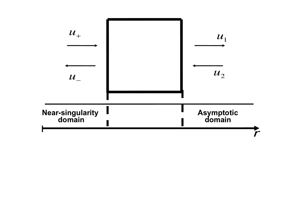
Figure 1: The multichannel framework can be visualized as a connector between two domains, each involving a singular point: the asymptotic domain ($r\sim\infty$), with outgoing/ingoing basis functions ${\bf u_{1}}$ and ${\bf u_{2}}$, and the near-singularity domain ($r\sim 0$), with outgoing/ingoing basis functions ${\bf u_{+}}$ and ${\bf u_{-}}$.

provide a formal solution to the most general problem of SQM with one finite singular point, as sketched in Fig. 1. In summary, the connection between the bases ${\mathcal{B}}_{\rm sing}$ and ${\mathcal{B}}_{\rm asymp}$ constitutes a two-channel framework, where each “channel” is associated with a singular point (with one finite singular point and the second singular point located at infinity)—generalizations to multiple singularities are possible as a multichannel setup Smatrix-singularQM , as will be further discussed elsewhere.

In particular, it is convenient to rewrite the distinct sides of Eq. (4) as

$$u(r)\propto\Omega\,u_{+}(r)+u_{-}(r)\;$$ (5)

and

$$u(r)\propto\hat{S}_{\rm asymp}\,u_{1}(r)+u_{2}(r)\;.$$ (6)

Here, with the use of the proportionality symbol, the ratio

$$\Omega=\frac{C^{\mbox{\tiny$(+)$}}}{C^{\mbox{\tiny$(-)$}}}\;$$ (7)

provides a “singularity parameter” related to the indeterminacy of the boundary conditions at the finite singular point. Thus, $\Omega$ specifies an auxiliary “boundary condition,” i.e., it gauges the relative probability amplitudes of outgoing (emission) to ingoing (absorption) waves in the neighborhood of $r=0$. Similarly, we fix the normalization for the point at infinity with

$$S_{\rm asymp}=e^{i\pi\left(l+\nu\right)}\,\hat{S}_{\rm asymp}\;,$$ (8)

in terms of the reduced matrix elements $\hat{S}_{\rm asymp}$ and an $l$- and $d$-dependent phase factor. Equations (6) and (8) yield the S-matrix from which the physical observables are extracted. In addition, by the way they are constructed as outgoing/ingoing waves, the basis functions satisfy

$$[u_{1}(r)]^{*} =u_{2}(r)\;,$$ (9)

$$[u_{+}(r)]^{*} =u_{-}(r)\;,$$ (10)

for $r\in\mathbb{R}$.

For the sake of completeness, we provide explicit expressions for the dominant behavior of the “singularity basis” Smatrix-singularQM ,

$$u_{\pm}(r)\stackrel{{\scriptstyle(r\rightarrow 0)}}{{\sim}} \frac{r^{p/4}}{{\lambda}^{1/4}}\,\exp\!\left[\mp 2\,i\,{\lambda}^{1/2}\,\frac{r^{-\left(p/2-1\right)}}{\left(p-2\right)}\right] p>2$$ for   , (11)

$$u_{\pm}(r)\stackrel{{\scriptstyle(r\rightarrow 0)}}{{\sim}} {\displaystyle\sqrt{\frac{r}{\Theta}}\,\exp\!\left[\pm i\,\Theta\,\ln\left(\mu r\right)\right]}=\sqrt{\frac{r}{\Theta}}\;\left(\,\mu\,r\,\right)^{\pm i\,\Theta} p=2$$ for   . (12)

Here, the normalization is also enforced with the WKB amplitude factor $(k_{\rm WKB})^{-1/2}$, see again further details in Sec. III. Moreover, the arbitrary floating inverse length $\mu$ for the regular singular case $p=2$, which is mandatory by its asymptotic conformal invariance, arises from the integration constant in the WKB solution or via dimensional homogeneity in the associated Cauchy-Euler differential equation. However, for the irregular singular case $p>2$, the integration constant in the exponent only appears at a higher order in the asymptotic expansion with respect to $1/r$; specifically, the Bessel-function solutions of Eq. (1) as $r\rightarrow 0$, $u/\sqrt{r}\propto H^{(1,2)}_{-1/n}\left(-2\sqrt{\lambda}\,r^{-n/2}/n\right)$, where $n=p-2>0$, combined with the asymptotics of Hankel functions, provide the correct outgoing/incoming behavior of Eq. (11). In addition, the conformal case $p=2$ includes the Langer correction Langer corresponding to the critical coupling $\lambda=1/4$, with shifted square-root coupling constant $\Theta^{2}\equiv\lambda-1/4$; in this case, for particular instances of nonrelativistic quantum mechanics, the angular momentum is merged with the marginally singular $p=2$ term at the same order, leading to an effective interaction coupling—but this does not occur for quantum fields in black hole backgrounds and other relativistic applications Smatrix-singularQM ; HEC-CQManomaly1 ; HEC-CQManomaly2 ; HEC:CQM-renormalization . Parenthetically, when the potential has a long-range tail for $r\sim\infty$ given by $V(r)\sim-\lambda r^{-\delta}$, the asymptotic behavior involves an extra phase in the form $\sqrt{k}\,u_{1,2}(r)\stackrel{{\scriptstyle(r\rightarrow\infty)}}{{\sim}}\,e^{\mp i\pi/4}\,e^{\pm ikr}\,e^{\pm i\lambda r^{1-\delta}/2k(1-\delta)}$ which can be similarly derived by WKB integration for the irregular singular point at infinity Smatrix-singularQM .

III Analytic Structure of the S-matrix

For the remainder of this paper, we will write the reduced asymptotic S-matrix, defined by Eq. (6), as $\hat{S}\equiv\hat{S}_{\rm asymp}$. The S-matrix of physical interest follows from Eq. (8). From Sec. II, the existence of a complex function

$$\hat{S}=\hat{S}(\Omega)$$

of the variable $\Omega$ relies on the singular nature of the potential via Eqs. (5) and (6). Specifically, the boundary condition indeterminacy at the finite singular point (e.g., the origin) is described by the arbitrary parameter $\Omega$ that represents the ratio of the amplitude coefficients for the required outgoing and ingoing waves at the singularity. By the nature of the solutions, $\Omega$ is generically a complex number.

In addition, $\hat{S}(\Omega)$ is a meromorphic function, as follows constructively from the definition of the “parameters” $\hat{S}$ and $\Omega$ in the scattering process. In effect, the linear relationship between the coefficients $(C^{\mbox{\tiny$(+)$}},C^{\mbox{\tiny$(-)$}})$ and $(C^{\mbox{\tiny$(1)$}},C^{\mbox{\tiny$(2)$}})$, or between the corresponding bases, as displayed by Eq. (4), implies a fractional linear transformation for the relationship between $\hat{S}$ and $\Omega$. Thus, properties of Möbius functions can be used to further understand this formalism Smatrix-singularQM . By contrast, in this paper, we reverse the logic and focus on the basic principles that ultimately generate this remarkable analytic structure of the S-matrix for singular potentials.

The central results we address below are based on the analytic structure of the S-matrix that relies on Blaschke factorization. For our current purposes, some language, properties, and theorems of Blaschke products are in order. Let $\mathbb{D}=\left\{\Omega\in\mathbb{C}:\;\;|\Omega|<1\right\}$ and $\overline{\mathbb{D}}=\left\{\Omega\in\mathbb{C}:\;\;|\Omega|\leq 1\right\}$ be the open and closed unit disks in the complex plane, respectively; and the boundary $\mathbb{T}=\left\{\Omega\in\mathbb{C}:\;\;|\Omega|=1\right\}=\partial\overline{\mathbb{D}}$ be the unit circle. Then Blaschke1 ; Blaschke2 ,

Let $F(z)$ be a holomorphic function on $\mathbb{D}$ that can be extended to a continuous function on $\overline{\mathbb{D}}$. If $F$ is a mapping of the unit disk $\overline{\mathbb{D}}$ to itself that preserves the disk boundary $\mathbb{T}$ (i.e., $|F|=1$ if $|z|=1$), then $F$ admits a finite Blaschke product factorization,

$$F(z)=\zeta\;\prod_{j=1}^{n}\left(\frac{z-z_{j}}{1-z_{j}^{*}\,z}\right)\;,$$ (13)

where $\zeta$ is a phase factor ($|\zeta|=1$) independent of $z$ and $z_{j}$ are the zeros of $F(z)$ in $\mathbb{D}$.

For the case when a bounded analytic function satisfies the conditions above on the open disk $\mathbb{D}$, Carathéodory’s theorem yields a possibly infinite factorization with an appropriate behavior of the given sequence of zeros Garnett:1981 . In the finite case above, the number $n$ is the degree, ${\rm deg}\,F$, of the mapping.

Specifically, for our generic treatment of SQM, the mapping $\hat{S}(\Omega)$ is indeed restricted to the closed unit disk, $\overline{\mathbb{D}}$, i.e., $|S|\leq 1$ iff $|\Omega|\leq 1$. This property can be established directly from “conserved currents” (with the usual probabilistic interpretation in the particular case of quantum mechanics proper applications) as described by Wronskian properties of pairs of solutions of the governing differential equation. In effect, from the Wronskian $W[\psi_{1},\psi_{2}]$ of any two solutions of Eq. (1) (and/or their complex conjugates, which are also solutions), and through the definition $J[u]=W[u^{*},u]/i$ of conserved currents, it follows that $J[u_{\pm}]=\pm 2$ and similarly $J[u_{1,2}]=\pm 2$ (guaranteed by the WKB normalization). More generally, the form $J[u,v]=W[u^{*},v]/i$ is conjugate-symmetric sesquilinear, $J[u,\lambda_{1}v_{1}+\lambda_{2}v_{2}]=\lambda_{1}J[u,v_{1}]+\lambda_{2}J[u,v_{2}]$ and $\left(J[u,v]\right)^{*}=J[v,u]$, and further satisfies $\left(J[u,v]\right)^{*}=-J[u^{*},v^{*}]$. Then, from these definitions, one can derive all the relevant current-conservation relations, including explicit identities for reflection and transmission coefficients. Moreover, the Hermitian quadratic form $J[u]\equiv J[u,u]$ is an SU(1,1) inner product in the specific sense that $J[u^{*}]=-J[u]$, leading to $J[\lambda_{1}u+\lambda_{2}u^{*}]=\left(|\lambda_{1}|^{2}-|\lambda_{2}|^{2}\right)\,J[u]$; thus, for wave function (4) that is the general solution to Eq. (1),

$$\frac{1}{2}\,J[u]=|C^{(1)}|^{2}-|C^{(2)}|^{2}=|C^{(+)}|^{2}-|C^{(-)}|^{2}\;.$$ (14)

This implies that $\bigl{|}\hat{S}\bigr{|}^{2}-1=\left[\left|\Omega\right|^{2}-1\right]\,|C^{(-)}/C^{(2)}|^{2}$, whence

$${\rm sgn}\left(J\right)={\rm sgn}\left[\bigl{|}\hat{S}\bigr{|}^{2}-1\right]={\rm sgn}\left[\left|\Omega\right|^{2}-1\right]\;.$$ (15)

Therefore, $\bigl{|}\hat{S}\bigr{|}\leq 1$ iff $\left|\Omega\right|\leq 1$ (with one-to-one correspondence of the equal signs), so that from the ensuing map $\hat{S}(\Omega)$ one concludes that $\hat{S}(\Omega)$ admits the Blaschke factorization (13), with $z\equiv\Omega$ and $F\equiv\hat{S}$, up to a global phase.

The characterization of the form of the asymptotic S-matrix concludes with the restriction to a single Blaschke factor, which is due to the existence of a unique zero $\Omega_{1}={\mathcal{R}}^{*}$ for the S-matrix (except for $|\mathcal{R}|=1$; see below). This property can be established from general arguments, as follows. First, from the generic framework of Sec. II, one can depict the zeros and poles of the S-matrix using Fig. 1. In effect, the zero of $\hat{S}$ occurs when the building block $u_{1}$ is suppressed. Second, define the solutions $\check{u}_{1}$ and $\check{u}_{-}$, with modified normalizations adapted to the standard 1D scattering problem,

$$\check{u}_{1} = \left\{\begin{array}[]{ll}u_{+}+{\mathcal{R}}u_{-}&\;\;{\rm for}\;r\sim 0\\ {\mathcal{T}}u_{1}&\;\;{\rm for}\;r\sim\infty\end{array}\right.\;,$$ (18)

$$\check{u}_{-} = \left\{\begin{array}[]{ll}u_{2}+{\mathcal{R}^{\prime}}u_{1}&\;\;{\rm for}\;r\sim\infty\\ {\mathcal{T}^{\prime}}u_{-}&\;\;{\rm for}\;r\sim 0\end{array}\;,\right.$$ (21)

where $({\mathcal{R}},{\mathcal{T}})$ and $({\mathcal{R}}^{\prime},{\mathcal{T}}^{\prime})$ are, respectively, the right-moving and left-moving reflection and transmission amplitude coefficients. Third, by time-reversal invariance (given by the complex conjugate and reversal of the arrows in Fig. 1), we can see that this amounts to $\check{u}_{1}^{*}=\left({\mathcal{T}}u_{1}\right)^{*}={\mathcal{T}}^{*}u_{2}$, where Eq. (9) was used—this effectively suppresses $u_{1}$ and selects the zero of $\hat{S}$; thus, $\check{u}_{1}^{*}=[u_{+}]^{*}+{\mathcal{R}}^{*}[u_{-}]^{*}=u_{-}+{\mathcal{R}}^{*}u_{+}$, leading to

$$\Omega_{1}=\left.\Omega\right|_{\rm zero\;of\;\hat{S}}={\mathcal{R}}^{*}\;$$ (22)

[by comparison against Eq. (5)]. Fourth, from the physical bound $|{\mathcal{R}}|\leq 1$, which is established through $|{\mathcal{R}}|^{2}+|{\mathcal{T}}|^{2}=1$ via Wronskian relations (see below), it follows that

for $$|{\mathcal{R}}|<1 \Omega_{1}={\mathcal{R}}^{*} \Omega_{1}\in{\mathbb{D}}$$, there is a unique zero of the S-matrix, with . (23)

So far, we have only established that $\Omega_{1}\in\overline{\mathbb{D}}$, but a zero on the unit circle $\mathbb{T}=\partial\overline{\mathbb{D}}$ is to be rejected, as shown below. Fifth, by comparison against Eq. (13), one can explicitly write the reduced S-matrix as a single Blaschke factor times a global phase,

$$\hat{S}=\Delta\,\frac{\Omega-{\mathcal{R}}^{*}}{{\mathcal{R}}\,\,\Omega-1}\;.$$ (24)

Sixth, regarding the general Blaschke-factor of Eq. (24), when $|\mathcal{R}|=1$, the S-matrix is trivial with respect to $\Omega$, in the sense that it is restricted to the unit circle, $|\hat{S}|=1$ and $\Omega$-independent, as can be easily verified (this is a general property of the Blaschke factors); thus, in that case, being a constant, $\hat{S}$ has neither zeros nor poles—incidentally, there is no contradiction herein because $\mathcal{T}=0$ when $|\mathcal{R}|=1$, and the asymptotic form of Eq. (18) becomes degenerate, failing to produce an actual zero of $\hat{S}$. Finally, in Eq. (24), it is also possible to identify the global phase as

$$\Delta=-\frac{{\mathcal{T}}}{{\mathcal{T}}^{*}}=\frac{{\mathcal{R}^{\prime}}}{{\mathcal{R}}^{*}}\;,$$ (25)

from the following general arguments: (i) $\Delta={\mathcal{R}^{\prime}}/{\mathcal{R}}^{*}$ from $\hat{S}(\Omega=0)={\mathcal{R}^{\prime}}$ (i.e., the corresponding S-matrix is the left-moving reflection coefficient); (ii) by means of a Wronskian relation, the Stokes’ reciprocity relation ${\mathcal{T}}{\mathcal{R}}^{*}+{\mathcal{T}}^{*}{\mathcal{R}^{\prime}}=0$ is established. Parenthetically, a network of Wronskian relations $W\bigl{[}\check{u}_{1}^{*},\check{u}_{1}\bigr{]}$, $W\bigl{[}\check{u}_{-}^{*},\check{u}_{-}\bigr{]}$, $W\bigl{[}\check{u}_{1}^{*},\check{u}_{-}\bigr{]}$, and $W\bigl{[}\check{u}_{1},\check{u}_{-}\bigr{]}$, implies the following four conditions: $|{\mathcal{R}}|^{2}+|{\mathcal{T}}|^{2}=1$, $|{\mathcal{R}^{\prime}}|^{2}+|{\mathcal{T}^{\prime}}|^{2}=1$, ${\mathcal{R}^{*}}{\mathcal{T}^{\prime}}+{\mathcal{T}^{*}}{\mathcal{R}^{\prime}}=0$, and ${\mathcal{T}^{\prime}}={\mathcal{T}}$ (with the last two being used in the above argument).

It should be noticed that various particular cases of Eq. (24) have appeared in the literature in Refs. perelomov:70 ; Alliluev_ISP ; aud:99 (for $\Omega=0$) and in Ref. Voronin (for $\Omega=0$ and $\Omega=\infty$), while the general form has been derived by other techniques in Refs. Esposito ; Stroffolini ; Smatrix-singularQM .

As a corollary of relations (23)–(25),

the function $\hat{S}(\Omega)$ is analytic in the closed unit circle $\overline{\mathbb{D}}$, i.e., it is a meromorphic function with no poles for $|\Omega|\leq 1$.

This is simply due to the fact that the unique purported pole is located at $\Omega_{2}=1/{\mathcal{R}}$, as shown by the Blaschke factor—but this location of $\Omega_{2}$ could also be established independently by a similar subset of arguments, via the suppression of the building block $u_{2}$ combined with Eq. (18) leading to $\check{u}_{1}=u_{+}+{\mathcal{R}}u_{-}$ (i.e, $\Omega$ given by the explicit ratio $\Omega_{2}=1/\mathcal{R}$). Thus, by a reversal of the reflection-coefficient bound discussed above, $|\Omega_{2}|=|1/{\mathcal{R}}|=1/|\Omega_{1}|\geq 1$; in addition, the trivial case $|{\mathcal{R}}|=1$ can be dealt with separately [as established in the argument following Eq. (24)], thus leading to $\hat{S}$ being a constant ($\Omega$-independent) of modulus one, so that the stricter condition $|\Omega_{2}|>1$ is enforced.

Incidentally, the S-matrix of Eq. (24), being a single Blaschke factor, defines a well-known Möbius transformation $\hat{S}(\Omega)$ that is an automorphism of the unit disk Needham_Complex .

IV Determination of Nonunitary Solutions from the Whole Family of Unitary Solutions

The general properties discussed in Sec. III for the two-channel case (with one singularity other than asymptotic infinity) yield a holomorphic function $\hat{S}(\Omega)$ with a unique zero at $\Omega_{1}=\mathcal{R}^{*}$. Furthermore, the scattering bound $|{\mathcal{R}}|\leq 1$ (familiar restriction on the reflection coefficients) leads to a location of the corresponding pole outside the unit disk $\mathbb{D}$, so that the function $\hat{S}(\Omega)$ is guaranteed to be analytic in $\overline{\mathbb{D}}$ (i.e., $|\Omega|\leq 1$).

As a result, Cauchy’s integral formula Needham_Complex implies the following “average characterization” of nonunitary solutions for all the cases with absorption due to a singular potential,

$$\hat{S}(\Omega)=\frac{1}{2\pi i}\oint\limits_{{\mathbb{T}}}d\Omega^{\prime}\,\frac{\hat{S}(\Omega^{\prime})}{\Omega^{\prime}-\Omega}\;,$$ (26)

where $\mathbb{T}=\partial\overline{\mathbb{D}}$ is the unit circle consisting of the whole family of unitary S-matrix values, i.e., the whole family of solutions to Eq. (1) with “elastic” or self-adjoint boundary conditions. This amounts to $\Omega^{\prime}=e^{i\chi}$, where $\chi\in\mathbb{R}$ is a phase specifying the generic self-adjoint condition. The one-to-one correspondence of the conditions $|\Omega^{\prime}|=1$ and $|S(\Omega^{\prime})|=|\hat{S}(\Omega^{\prime})|=1$ can be seen from Eq. (15). With this notation, and going back to the primitive form of asymptotic S-matrix (8) by reintroducing the required phase factors (whenever appropriate), Eq. (26) can be rewritten in the suggestive form

$${S}(\Omega)=\int_{0}^{2\pi}\frac{d\chi}{2\pi}\;\frac{{S}(\Omega^{\prime}=e^{i\chi})}{1-\Omega\,e^{-i\chi}}\;.$$ (27)

Equation (27) is an ensemble average with a nonuniform (shifted) weight of the whole family of unitary S-matrices. Therefore, we have established the general identity relating unitary and nonunitary solutions for $|\Omega|<1$, i.e., all the cases that exhibit net absorption.

The particular case of “perfect absorption,” $\Omega=0$, involves a symmetric ensemble average with uniform weight, i.e.,

$${S}(\Omega=0)=\int_{0}^{2\pi}\frac{d\chi}{2\pi}\;{S}(\Omega^{\prime}=e^{i\chi})\;,$$ (28)

which corresponds to the particular case considered in Refs. radin:75 and bawin_coon_wire . It is also noteworthy that this is equal to the left-moving reflection coefficient: $\hat{S}(\Omega=0)={\mathcal{R}}^{\prime}$ [see Eqs. (24) and (25)]. Our present work shows that this result is not accidental but the logical consequence of general physical principles applied to the S-matrix—following a similar methodology to the S-matrix approach in field theory. Remarkably, this is a generic property of SQM (either conformal or an irregular singularity): while singular potentials support this analytic “structure,” the distinct case (not tackled herein) of absorption by complex (optical) potentials generally does not.

V Conclusions

We have shown that, given the existence of a singular problem (in the sense of SQM), a basic set of general principles: linearity, unitarity of the multichannel S-matrix with the related network of current-conservation statements (encoded by reflection and transmission coefficients), and time-reversal symmetry allow the complete determination of the analytic structure of the asymptotic S-matrix of SQM with respect to the parameter $\Omega$ that specifies boundary conditions. This analytic structure involves Möbius transformations of the Blaschke-factor type associated with the unit disk. Due to its generality, this approach also provides the rationale to predict and explain the intriguing average relationship between unitary and nonunitary solutions at the level of the asymptotic S-matrix.