Thesis
Coronal upflows from edges of an active region observed with EUV Imaging Spectrometer onboard Hinode

© Naomasa Kitagawa, 2014

Abstract

In order to better understand the plasma supply and leakage at active regions, we investigated physical properties of the upflows from edges of active region NOAA AR10978 observed with the EUV Imaging Spectrometer (EIS) onboard Hinode. Our observational aim is to measure two quantities of the outflows: Doppler velocity and electron density.

These upflows in the corona, referred to as active region outflows (hereafter the outflows), were discovered for the first time by EIS due to its unprecedented high sensitivity and spectral resolution. Those outflows are emanated at the outer edge of a bright active region core, where the intensity is low (i.e., dark region). It is well known by a number of EIS observations that the coronal emission lines at the outflow regions are composed of an enhanced component at the blue wing (EBW) corresponding to a speed of $\sim 100\,\mathrm{km}\,\mathrm{s}^{-1}$, added to by the stronger major component almost at rest. This EBW can be seen in line profiles of Fe xii–xv whose formation temperatures are around $\log T\,[\mathrm{K}]=6.2\text{--}6.3$. It has been suggested that the outflows are (1) an indication of upflows from the footpoints of coronal loops induced by impulsive heating in the corona, (2) induced by the sudden pressure change after the reconnection between closed active region loops and open extended loops located at the edge of an active region, (3) driven by the contraction occurring at the edge of an active region which is caused by horizontal expansion of the active region, and (4) the tips of chromospheric spicules heated up to coronal temperature. While a number of observations have been revealed such aspects of the outflows, however, their electron density has not been known until present, which is one of the important physical quantities to consider the nature of the outflows. In addition, the Doppler velocity at the transition region temperature ($\log T\,[\mathrm{K}]\leq 6.0$) has not been measured accurately in the outflow regions because of the difficulties in EIS spectroscopic analysis (e.g., the lack of onboard calibration lamp for absolute wavelength, and the temperature drift of line centroids according to the orbital motion of the satellite). In this thesis, we analyzed the outflow regions in NOAA AR10978 in order to measure Doppler velocity within wide temperature range ($\log T\,[\mathrm{K}]=5.5\text{--}6.5$) and electron density by using an emission line pair Fe xiv $264.78$Å/$274.20$Å.

Since EIS does not have an absolute wavelength reference onboard, we need another reference for the precise measurement of the Doppler velocity. In this thesis, we exploited Doppler velocity of the quiet region as the reference, which was studied in Chapter 3. EUV emission lines observed in the quiet region are known to indicate redshift corresponding to $v\simeq 10\,\mathrm{km}\,\mathrm{s}^{-1}$ at $\log T\,[\mathrm{K}]\leq 5.8$, while those above that temperature have not been established where a number of emission lines observed with EIS exist. Since the corona is optically thin, spectra outside the limb are superposed symmetrically along the line of sight, which leads to the reasonable idea that the limb spectra take a Doppler velocity of $v=0$. We derived the Doppler velocity of the quiet region at the disk center by studying the center-to-limb variation of line centroid shifts for eleven emission lines from the transition region and the corona. By analyzing the spectroscopic data which cover the meridional line of the Sun from the south pole to the north pole, we determined the Doppler velocity of the quiet region with $5.7\leq\log T\,[\mathrm{K}]\leq 6.3$ in the accuracy of $\simeq 3\,\mathrm{km}\,\mathrm{s}^{-1}$ for the first time. It is shown that emission lines below $\log T\,[\mathrm{K}]=6.0$ have Doppler velocity of almost zero with an error of $1\text{--}3\,\mathrm{km}\,\mathrm{s}^{-1}$, while those above that temperature are blueshifted with gradually increasing magnitude: $v=-6.3\pm 2.1\,\mathrm{km}\,\mathrm{s}^{-1}$ at $\log T\,[\mathrm{K}]=6.25$.

The Doppler velocity of the outflows was measured for twenty six emission lines which cover the temperature range of $5.5\leq\log T\,[\mathrm{K}]\leq 6.5$ in Chapter 4. Though it is well known that the outflows are prominent around $\log T\,[\mathrm{K}]=6.1\text{--}6.3$ and exhibit clear blueshift corresponding to several tens of $\mathrm{km}\,\mathrm{s}^{-1}$ due to the existence of EBW extending up to $\sim 100\,\mathrm{km}\,\mathrm{s}^{-1}$, the behavior below that temperature has not been revealed. Using the Doppler velocity of the quiet region (obtained in Chapter 3) for the temperature range of $5.7\leq\log T\,[\mathrm{K}]\leq 6.3$ as a reference, we measured the Doppler velocity of several types of coronal structures in NOAA AR10978: active region core, fan loops, and the outflow regions. Active region core, characterized by high temperature loops ($\log T\,[\mathrm{K}]\geq 6.3\text{--}6.4$), indicated almost the same centroid shifts as the quiet region selected in the field of view of the EIS scan. Fan loops are extending structures from the periphery of active regions, which indicated $v\simeq 10\,\mathrm{km}\,\mathrm{s}^{-1}$ at the transition region temperature, and the Doppler velocity decreased with increasing formation temperature: reaching $v=-20\,\mathrm{km}\,\mathrm{s}^{-1}$ at $\log T\,[\mathrm{K}]=6.3$. Different from fan loops, the outflow regions exhibited a blueshift corresponding to $v\simeq-20\,\mathrm{km}\,\mathrm{s}^{-1}$ at all temperature range below $\log T\,[\mathrm{K}]=6.3$, which implies that the plasma does not return to the solar surface. The fact that the outflow region and fan loops are often located near each other has been made it complicated to understand the physical view of those structures. By extracting the target regions with much carefulness, we revealed the definitive difference of the outflow regions and fan loops in the Doppler velocity at the transition region temperature.

In Chapter 5, the electron density of the outflows (EBW component in coronal emission line profiles) was derived for the first time by using a density-sensitive line pair Fe xiv $264.78$Å/$274.20$Å. This line pair has a wide sensitivity for the electron density range of $n_{\mathrm{e}}=10^{8\text{--}10}\,\mathrm{cm}^{-3}$, which includes the typical values in the solar corona. We extracted EBW component from the line profiles of Fe xiv through double-Gaussian fitting. Since those two emission lines are emitted from the same ionization degree of the same ion species, they should be shifted by the same amount of Doppler velocity and thermal width. We challenged the simultaneous fitting applied to those two Fe xiv lines with such physical restrictions on the fitting parameters. After the double-Gaussian fitting, we obtained the intensity ratio of Fe xiv $264.78$Å/$274.20$Å both for the major component and EBW component. Electron density for both component ($n_{\mathrm{Major}}$ and $n_{\mathrm{EBW}}$) was calculated by referring to the theoretical intensity ratio as a function of electron density which is given by CHIANTI database. We studied six locations in the outflow regions. The average electron density in those six locations was $n_{\mathrm{Major}}=10^{9.16\pm 0.16}\,\mathrm{cm}^{-3}$ and $n_{\mathrm{EBW}}=10^{8.74\pm 0.29}\,\mathrm{cm}^{-3}$. The magnitude relationship between $n_{\mathrm{Major}}$ and $n_{\mathrm{EBW}}$ was different in the eastern and western outflow regions, which was discussed in Section 7 associated with the magnetic topology. The column depth was also calculated by using the electron densities for each component in the line profiles, and it leads to the result that (1) the outflows possess only a small fraction ($\sim 0.1$) compared to the major rest component in the eastern outflow region, while (2) the outflows dominate over the rest plasma by a factor of around five in the western outflow region.

We developed a new method in line profile analysis to investigate the electron density of a minor component in Chapter 6. Instead of obtaining the electron density from the intensity ratio calculated by the double-Gaussian fitting, we derive the electron density for each spectral bin in Fe xiv line profiles, which we refer to as $\lambda$-$n_{\mathrm{e}}$ diagram. This method has an advantage that it does not depend on any fitting models. By using the $\lambda$-$n_{\mathrm{e}}$ diagram, we confirmed that EBW component indeed has smaller electron density than that of the major component in the western outflow region while that was not the case in the eastern outflow region.

Our implications are as follows.

(1) The outflow regions and fan loops, which has been often discussed in the same context, exhibited different temperature dependence of Doppler velocity. We concluded these structures are not identical.

(2) We tried to interpret the outflows in terms of the siphon flow (i.e., steady and unidirectional) along coronal loops, but it turned out to be unreasonable because both the mass flux and the gas pressure gradient were in the opposite sense to what should be expected theoretically.

(3) The temperature dependence of the Doppler velocity in the outflow regions are different from that was predicted by a previous numerical simulation on impulsive heating with longer timescale than the cooling. We observed upflow at the transition temperature, while the numerical simulation resulted in downflow at that temperature.

(4) As for the case if intermittent heating is responsible for the outflows, we analytically considered a balance between heating and the enthalpy flux. The duration of heating was crudely estimated to be longer than $\tau=500\,\mathrm{s}$ so that the density of upflows from the footpoints becomes compatible with that of the observed outflows.

(5) Though EBW component contributes to the emission as a small fraction in a line profile, the volume amount is around five times as large as the major component in the western outflow region as calculated by using the electron density for each component in Fe xiv line profiles.

(6) Coronal loops rooted at the eastern outflow regions are connected to the opposite polarity region within the active region when taking into account the magnetic topology constructed from an MDI magnetogram, from which we suggest a possibility that the outflows actually contribute to the mass supply to active region coronal loops at the eastern outflow region.

Chapter 1 Introduction

1.1 The solar corona

The solar corona is an outer atmosphere of the Sun which has a temperature exceeding $10^{6}\,\mathrm{K}$. It is an outstanding issue how the corona can be heated up to so high temperature compared to the inner photosphere, where the temperature is around $6000\,\mathrm{K}$. The observations of the solar corona date back to ancient eclipse recorded by Indian, Babylonian and Chinese. Routine coronal observations started when Beonard Lyot built the first coronagraph in 1930, which occults the brighter photosphere by using a disk. Forbidden lines of highly ionized atoms (Fe x–xiv; Ni xii–xvi) were identified (Edlén 1943; Swings 1943) and it was claimed for the first time that the coronal temperature exceeds million Kelvin ($\mathrm{MK}$). As already mentioned, the physical explanation of the mechanism keeping this high temperature in the solar corona is still unknown. The second law of thermodynamics seems to be violated in the point that the much cooler photosphere ($T\sim 6000\,\mathrm{K}$) exists at inner atmosphere, closer to the energy source at the core of the star.

The temperature profile along the height is shown in Fig. 1.1, from which we can see the decreasing temperature in the photosphere and the increasing temperature from the bottom of the chromosphere where the temperature takes minimum value ($\sim 4200\,\mathrm{K}$), to the upper atmosphere. There is a thin layer called the transition region between the cool chromosphere ($\sim 10^{4}\,\mathrm{K}$) and the hot corona ($\geq 10^{6}\,\mathrm{K}$). It is appropriate to think this layer as a temperature regime rather than a geometric layer because of the extremely spatial inhomogeneous structure in the solar atmosphere. The density profile also has steep gradient while the pressure must be continuous through the transition region. In the upper part of the transition region the temperature reaches up to $10^{6}\,\mathrm{K}$. Due to the high temperature exceeding $10^{6}\,\mathrm{K}$, the corona consists of ions with high degree of ionization. These ions efficiently radiate the line emission in the EUV and X-ray wavelength range.

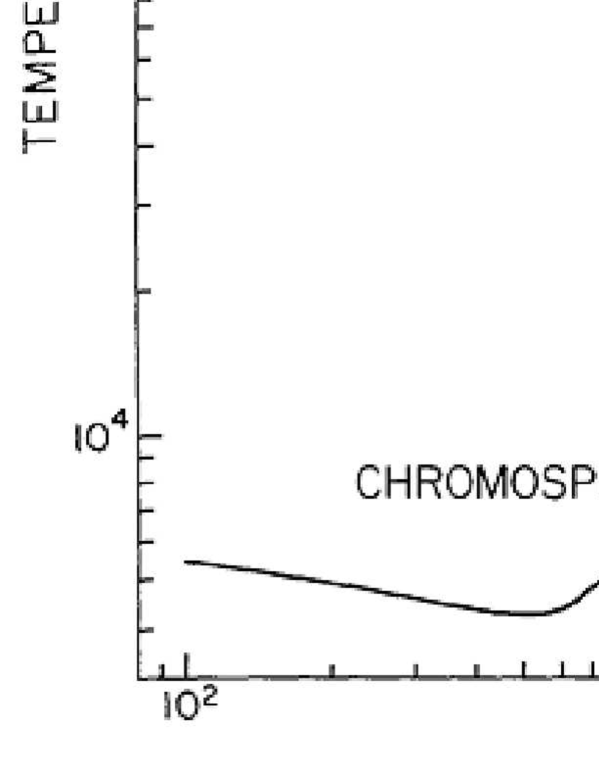
Fig. 1.1: Distribution of temperature (solid line) and hydrogen density (dashed line) in the solar atmosphere as a function of height from the photosphere $\tau_{5000}=1$. Excerpted from Withbroe & Noyes (1977).

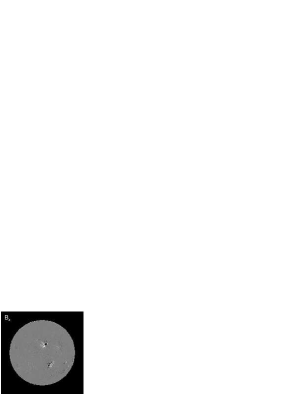
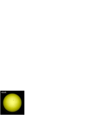
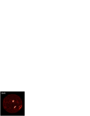
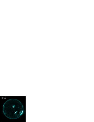
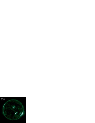
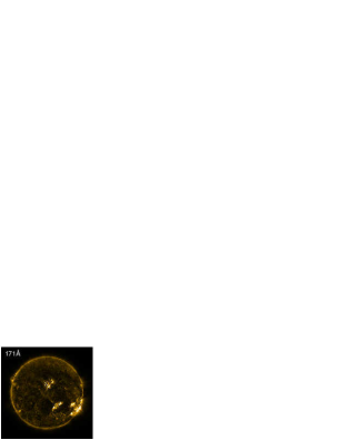
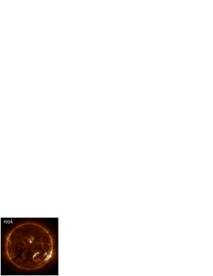
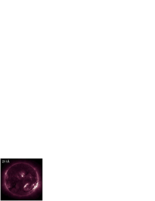
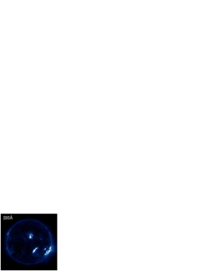
Fig. 1.2: Images taken by SDO on 2012 August 14. Right upper panel shows a magnetogram taken by HMI. Other panels show EUV images taken by AIA. Numbers at upper right in each panel represent the wavelength of passband. EUV images are displayed in an order of the formation temperature dominant in each filter.

The solar corona has been categorized into three kinds historically by its X-ray brightness: active region, the quiet region, and coronal hole. In Fig. 1.2, various appearances of the solar corona are seen in the images taken by different filters of Atmospheric Imaging Assembly (AIA) onboard Solar Dynamics Observatory (SDO) launched by NASA. There are several bright areas (active regions) slightly at the north of the center and in the south west. At the south east of the center, there is a dark region most clearly seen in the $193$Å passband image. Such a kind of region is called as a coronal hole. The location other than active regions and a coronal hole is the quiet region.

Active regions are located in areas of strong magnetic field concentrations, visible as sunspot groups in optical wavelengths and magnetograms. Sunspot groups typically exhibit a strongly concentrated leading magnetic polarity, followed by a more fragmented trailing group of opposite polarity. Because of this bipolar nature active regions are mainly made up of closed magnetic field lines. Due to the persistent magnetic activity in terms of magnetic flux emergence, flux cancellation, magnetic reconfigurations, and magnetic reconnection processes, a number of dynamic phenomena such as transient brightenings, flares, and coronal mass ejections occur in active regions. We focus the persistent upflow seen at the edge of active regions in this thesis, which was discovered by EUV Imaging Spectrometer (EIS) onboard Hinode.

Active regions are constructed by structures along the magnetic field, which has been called as “coronal loops”, since X-ray observations from the space have enabled us to see the loop appearance along the coronal magnetic field (Rosner et al. 1978). Due to the nature of the solar corona that the plasma beta is much smaller than unity ($\beta\ll 1$), and that thermal conduction is strongly constrained in the direction parallel to magnetic field, the structures seen in EUV or X-ray images are basically configurated by the magnetic field. A consequence of the plasma heating in the transition region and the chromosphere is the upflow into coronal part which makes the coronal loops filled with hotter and denser plasma than the background corona. Those coronal loops produce bright emission.

As an example of active region, a magnetogram taken by Heliospheric and Magnetic Imager (HMI) onboard SDO and two EUV images taken by SDO/AIA $171$Å ($\log T\,[\mathrm{K}]\simeq 5.9$) and $335$Å ($\log T\,[\mathrm{K}]\simeq 6.5$) passbands are shown in Fig. 1.3. The active region was extracted from near the center of the Sun shown in Fig. 1.2. An extended structure similar to a fan can be clearly seen at the east and west edge of the active region in the AIA $171$Å passband image (indicated by white characters), which is called “fan loops”. Fan loops are often clearly seen in EUV images corresponding to a temperature around $\log T\,[\mathrm{K}]\simeq 5.7$–$6.0$. In the AIA $335$Å passband image, there are multiple loop systems connecting the opposite polarities with strong magnetic field in the south east–north west direction as indicated by white characters. These loops form the dominant emission of the active region and are called as active region “core”.

The quiet region is the area outside active regions. It is relatively quiet, however, various kinds of small dynamic phenomena have been observed all over the quiet region today by virtue of high resolution, for example, explosive events, bright points, jets, and giant arcade eruptions. The faint areas are called “coronal holes”, where magnetic field lines are opened into the outer space. Thus, the coronal plasma can be ejected possibly as the solar wind. Frequently occurring soft X-ray jets have been observed by the previous Japanese satellite Yohkoh and X-ray telescope (XRT) onboard Hinode.

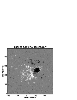
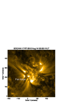
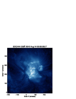
Fig. 1.3: Left: Magnetogram taken by SDO/HMI. Middle: EUV image taken by SDO/AIA $171$Å passband ($\log T\,[\mathrm{K}]\simeq 5.9$). Right: EUV image taken by SDO/AIA $335$Å passband ($\log T\,[\mathrm{K}]\simeq 6.5$).

1.2 Active region outflows

The flows in the solar corona play a crucial role in dynamics and formation of variable structures, and observations of their properties constrain the coronal heating problem. Observations on the flows in the solar corona are described here.

From observations by Solar Ultraviolet Measurements of Emitted Radiation (SUMER) onboard SoHO, spectra of the transition region lines ($\leq 10^{6}\,\mathrm{K}$) are known to be redshifted both in the quiet region and in an active region core (Chae et al. 1998; Peter & Judge 1999; Teriaca et al. 1999). On the other hand, coronal lines ($\simeq 10^{6}\,\mathrm{K}$) indicate blueshift. Hansteen et al. (2010) numerically showed that the redshift of transition region lines and slight blueshift of coronal lines are naturally produced by frequently occurring reconnections in the upper chromosphere as a response to the production of magnetic shear due to the braiding of magnetic fields by the photospheric convection. While those observations by SUMER focus on the low-temperature plasmas, the spectroscopic nature of the hotter component with $T\geq 10^{6}\,\mathrm{K}$ is still unclear, which is one of the main contents of this thesis (Chapter 3).

Flows have also been observed with imaging observations. Transition Region And Coronal Explorer (TRACE) had enabled a discover of persistent, intermittent flow pattern in coronal loops (Winebarger et al. 2001). Since there was no any obvious periodicity, it was concluded that the flow is induced by magnetic reconnection instead of the waves coming from the photosphere. The upward flows in coronal loops are also observed recently by AIA which has much higher temporal cadence than ever (full-Sun images at every $12\,\mathrm{s}$ for seven EUV wavelength bands), which revealed the ubiquitous existence of such flows in coronal loops extending from the edge of active regions (Tian et al. 2011).

1.2.1 Observations of AR outflows by Hinode/EIS

Spectral coverage sensitive to the coronal temperature and unprecedented high signal-to-noise ratio of Hinode/EIS enabled us to reveal the existence of upflows at the edge of active regions (Doschek et al. 2008; Hara et al. 2008; Harra et al. 2008). These upflows in the active region is called “AR (active region) outflows” and considered to be the upflows from the bottom of the corona. It has previously been confirmed that these outflows persist for several days in the images taken by X-Ray Telescope (XRT) onboard Hinode (Sakao et al. 2007). Some authors interpreted AR outflows as the source of the solar wind (Brooks & Warren 2011).

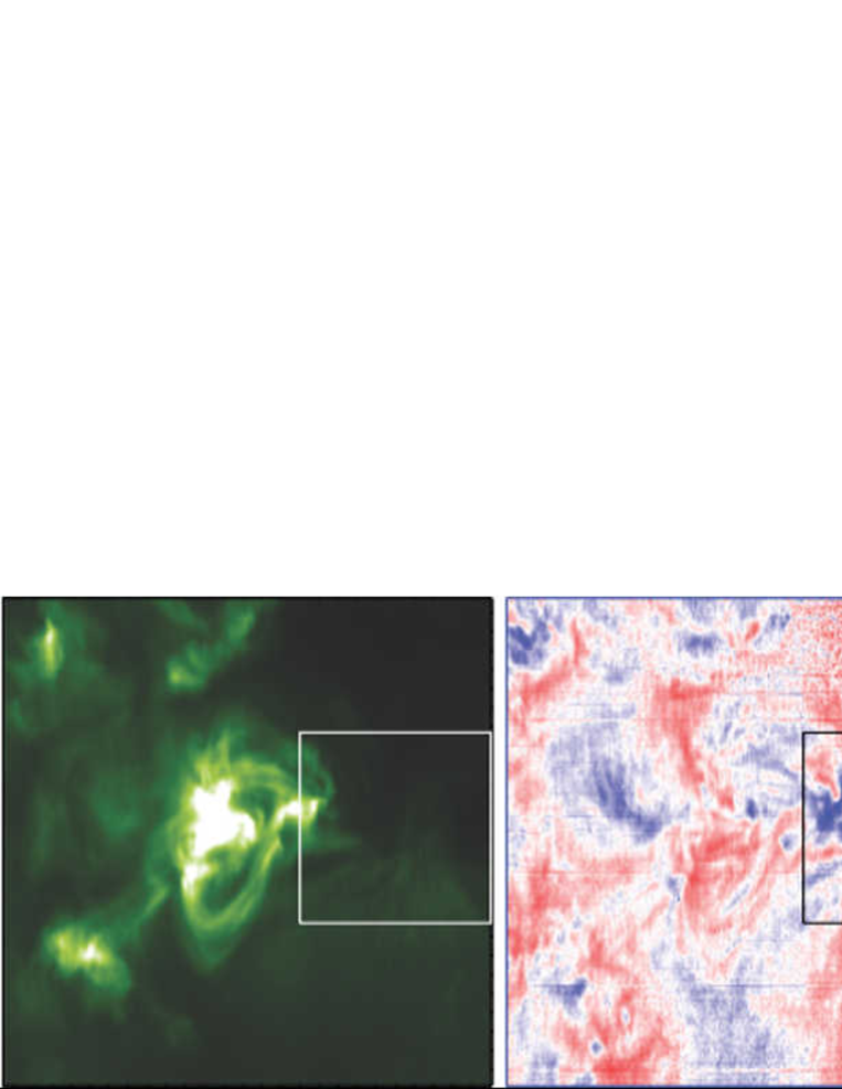
Fig. 1.4: Excerpts from Doschek et al. (2008). Right: Intensity map of Fe xii $195.12$Å for an active region taken on 2007 August 23. Left: Doppler velocity map. Blue (Red) indicates that the plasma moves toward (away) us.

Doschek et al. (2008) analyzed emission line profiles of Fe xii $195.12$Å and revealed that the outflows are observed at the dark region outside an active region core as seen in Fig. 1.4. A preliminary result from EIS has shown that there is a clear boundary between closed hot loops in the AR core ($\sim 3\times 10^{6}\,\mathrm{K}$) and extended cool loops ($\lesssim 1\times 10^{6}\,\mathrm{K}$) where the blueshift was observed (Del Zanna 2008). The upflows were seen in the low density and low radiance area. Meanwhile, redshift was observed in the AR core for all emission lines (Fe viii–xv). This apparent lack of signatures of any upflows at active region cores was explained as the situation that strong rest component in line profiles hinders the signal of upflows (Doschek 2012), but it has not been proved yet.

The magnetic configuration of the outflow region has been modeled by magnetic field extrapolation from the photospheric magnetogram (Harra et al. 2008; Baker et al. 2009), and it was revealed that AR outflows emanate from the footpoints of extremely long coronal loops in txhe edge of an active region (Harra et al. 2008). Close investigation revealed that AR outflows are located near the footpoints of quasi separatrix layers (QSLs), which forms the changes of the connectivity of the magnetic fields from closed coronal loops into open regions (Baker et al. 2009; Del Zanna et al. 2011).

The velocity of the outflow lies within the range of a few tens up to $\sim 100\,\mathrm{km}\,\mathrm{s}^{-1}$. These velocities were derived by subtracting the fitted single-Gaussian from raw line profiles (Hara et al. 2008), and by double-Gaussian fitting (Bryans et al. 2010). By using extrapolated magnetic fields, the real velocity was derived from Doppler velocity and found to have a speed of $60$–$125\,\mathrm{km}\,\mathrm{s}^{-1}$ (Harra et al. 2008). The upflow velocity of AR outflows increases with the formation temperature of which emission lines Si vii–Fe xv represent (Warren et al. 2011). The blueshift becomes larger in hotter emission line as $5\text{--}20\,\mathrm{km}\,\mathrm{s}^{-1}$ for Fe xii (formed at $\sim 1\times 10^{6}\,\mathrm{K}$) and $10\text{--}30\,\mathrm{km}\,\mathrm{s}^{-1}$ for Fe xv (formed at $\sim 3\times 10^{6}\,\mathrm{K}$) (Del Zanna 2008). The appearance of the blueshifted regions often seems to trace the loop-like structures, however, it is not completely understood whether the AR outflows are related to fan loop structures (Warren et al. 2011; Tian et al. 2011; McIntosh et al. 2012), which will be discussed later (Section 7.3).

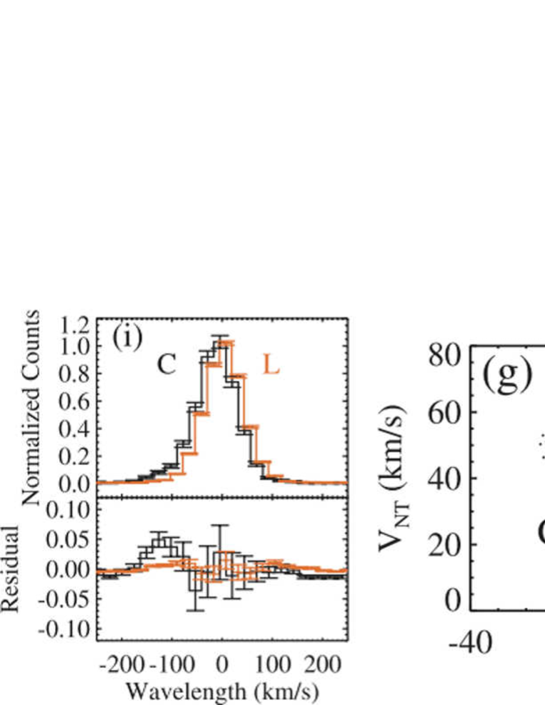
Fig. 1.5: Excerpts from Hara et al. (2008). Left: line profiles of Fe xiv $274.20$Å (top) and residuals from a fitted single Gaussian (bottom). Right: a scatter plot for Doppler and nonthermal velocities. C (black) and L (orange) in both panels respectively indicate the observation at the disk center and at the limb.

AR outflows are observed as an enhanced blue wing component (EBW) in the emission line profile of Fe xii–xv. An example for Fe xiv $274.20$Å is shown in the left panel of Fig. 1.5. By fitting the line profiles by a single Gaussian, it was revealed that there is a negative correlation between blueshifts and line widths (Doschek et al. 2008; Hara et al. 2008) as seen in the right panel of Fig. 1.5, which indicates the existence of unresolved component in the blue wing emitted from the upflowing plasma. Hara et al. (2008) investigated the line profile of Fe xiv and Fe xv ($\sim 2\times 10^{6}\,\mathrm{K}$) both at the disk center and at the limb (see black and orange plots in Fig. 1.5), and revealed that EBWs were clearly observed only at the disk center, which means that the upflow is dominantly in the radial direction as to the solar surface. This EBW does not exceed the major component at the rest by $\sim 25$% in terms of the intensity (Doschek 2012).

Observations so far have revealed properties of the outflow from the edge of active region such as (1) location: less bright region outside the edge of active region core, (2) magnetic topology: boundary between open magnetic fields and closed loops, and (3) the velocity: reaching up to $\sim 100\,\mathrm{km}\,\mathrm{s}^{-1}$ in the coronal temperature.

The velocity of the outflows in the transition region has not been investigated which becomes important because it decides whether the plasma in all temperature range including the transition region and the corona flows out from the region, which will be described in Section 4. In addition, the density of the outflow itself has not been investigated yet, which may be a crucial clue to reveal the driving mechanism (see the next section), and we will measure the density in Chapter 5.

1.2.2 Driving mechanisms of AR outflows

There are several types of driving mechanism of the AR outflow proposed so far. They are classified as (1) impulsive heating events concentrated at the footpoints of coronal loops (Hara et al. 2008; Del Zanna 2008), (2) the reconnection between open extended long loops located outside AR and inner loops (Harra et al. 2008; Baker et al. 2009), (3) horizontal expansion of active region (Murray et al. 2010), and (4) chromospheric spicules (McIntosh & De Pontieu 2009; De Pontieu et al. 2011).

Del Zanna (2008) interpreted that the upflow observed outside the active region core as gentle chromospheric evaporation induced by the reconnection (i.e., nanoflare) as a consequence of the braiding of magnetic footpoints at the photosphere, though the clear evidence has not been shown yet. While almost all of the observations on the outflow focus on the boundary where the magnetic topology changes (i.e., QSL), it was revealed that an upflow actually occurs at the footpoint of the closed active region loop (Hara et al. 2008). The existence of upflows with a speed up to $\simeq 100\,\mathrm{km}\,\mathrm{s}^{-1}$ in emission line profiles of Fe xiv $274.20$Å and xv $284.16$Å concentrated toward the footpoints was revealed, and that the line widths were also broadened. From those results, it was concluded that these observational results support the idea of impulsive heating of the lower corona (Serio et al. 1981; Aschwanden et al. 2000) instead of the uniform heating of corona loops (Rosner et al. 1978).

The outflows investigated so far tend to continue several days, from which some authors favor the interpretation of the driving mechanism in terms of interchange reconnection between the pre-existing long magnetic field in the quiet region and AR edge (Harra et al. 2008; Baker et al. 2009). Once the reconnection between closed loops and open field occurs, the dense plasma in the closed loops are no longer trapped, and accerelated by a pressure gradient and magnetic tension into the reconnected longer structure (Baker et al. 2009). One-dimensional hydrodynamic simulation showed that the rarefaction wave develops at the reconnected point where the jump in the pressure exists between hot core loop and much longer cool loop, which could produce observed velocity up to $50\,\mathrm{km}\,\mathrm{s}^{-1}$ and line width (Bradshaw et al. 2011). Their simulation also indicated the dependence of velocity on the temperature consistent with observations. However, the emission line profiles synthesized in their study were all symmetric, which differ from those observed at the outflow region (i.e., asymmetric and have a enhanced tail in their blue wing).

Among the driving mechanisms cited above, expansion of coronal loops (Murray et al. 2010) does not need the existence of magnetic reconnection. In their simulation, homogeneous magnetic field vertical to the solar surface was imposed at the initial. They set a strong magnetic flux tube with twist (which is much stronger than real AR) beneath the solar surface, which emerges from the interior of the Sun and expands until the magnetic pressure of the flux tube balances. The flux emergence is often observed in magnetograms, and it is regarded as the birth of an active region. Expanding tube pushes the initially existing atmosphere where the gas pressure increases due to the compression by the expanding tube. As a result, increased pressure forces the plasma to be accelerated up to $45\,\mathrm{km}\,\mathrm{s}^{-1}$ at the edge of expanding tube. However, there is one difficulty when trying to explain the persist nature of outflows. Their simulation only lasts for $25\,\mathrm{min}$, which is much shorter than the whole lifetime of an active region ($\sim\mathrm{month}$).

Different from other three mechanisms, McIntosh & De Pontieu (2009) and De Pontieu et al. (2011) suggested that the outflows are strongly coupled with chromospheric spicules. A small fraction at the tip of spicules observed with AIA was heated to temperature above $10^{6}\,\mathrm{K}$, and the propagating features were detected which have a speed of $\sim 50\text{--}100\,\mathrm{km}\,\mathrm{s}^{-1}$. These were interpreted as a counterpart of the outflows observed with Hinode/EIS. However, the heating mechanism of the tips of spicules has not mentioned.

1.3 Motivation

In this thesis, we focus on the outflow from the edge of active region which was discovered by Hinode/EIS. Main purpose is to clarify several aspects of the outflow region which have not been revealed yet: (1) Doppler velocity within a temperature range of $\log T\,[\mathrm{K}]=5.5$–$6.5$, and (2) the electron density. It has been already revealed that the fast upflow is seen in the coronal emission lines, but we do not precisely know the behavior of the transition region lines in the outflow region, which will be crucial information to understand the mass transport in the outflow region. The electron density may be a clue to understand the origin of the outflow and also can be used to evaluate the gas pressure. It helps us to consider how the outflow could be driven, combined with the magnetic field information.

This thesis is structured as follows. Two chapters following this introduction treat the preparation for the analysis. Chapter 2 is a brief introduction to the EIS instrument and the electron density diagnostics in emission line spectroscopy. The measurement of the spatially averaged Doppler velocity in the quiet region by investigating the center-to-limb variation of Doppler shift will be described in Chapter 3. After that measurement, the Doppler velocities of emission lines within a wide temperature range of $\log T\,[\mathrm{K}]=5.5$–$6.5$ were measured in the outflow region by referring the quiet region as zero-point of the Doppler velocity which will described in Chapter 4. The electron density of the AR outflow was derived in Chapter 5 by using a density-sensitive line pair Fe xiv $264.78$Å/$274.20$Å. Chapter 6 describes a new line profile analysis from a different point of view ($\lambda$-$n_{\mathrm{e}}$ diagram). We discuss the nature of the outflow region in Chapter 7. Finally, Chapter 8 will provide conclusions of this thesis. The potential magnetic field will be calculated around the active region in Appendix A, which helps us to consider the morphology of the outflow region.

Chapter 2 Diagnostics and instruments

2.1 Emission line spectroscopy

2.1.1 Spectral line profile

The corona, filled with highly ionized ions, produces line emissions in the extreme ultraviolet (EUV) wavelength range. There are several emission mechanisms such as bremsstrahlung, stimulated emission, spontaneous emission, radiative recombination, etc. In the coronal condition, the spontaneous emission dominates which makes an ion decaying from an upper level into a lower level. The most important process which causes the excitation from one energy level to upper level in the solar corona is inelastic collisions between ions and free electrons. Inelastic collisions are involved with almost all of the emission lines whose wavelength is shorter than $2000$Å. An electron-ion inelastic collision can be described as

$$X^{\,+m}_{i}(E_{i})+e(E_{1})\rightarrow X^{\,+m}_{j}(E_{j})+e(E_{2})\,\text{,}$$ (2.1)

where $i$ and $j$ indicate the initial and final levels of the ion $X^{\,+m}$, $E_{i}$ and $E_{j}$ are the initial and final energies, and $E_{1}$ and $E_{2}$ are the initial and final energies of the free electron. The ion in the final state can be de-excited spontaneously and emit one photon,

$$X^{\,+m}_{j}\rightarrow X^{\,+m}_{i}+h\nu_{ij}\,\text{,}$$ (2.2)

where $\nu_{ij}=(E_{j}-E_{i})/h$. Since the energy levels are discretized, a spectrum of an emission line has a sharp peak as a function of the frequency (i.e., also the wavelength). Fig. 2.1 shows an example of EUV spectra obtained by EUV Imaging Spectrometer (EIS) onboard Hinode. There are a number of peaks in the spectra emitted from highly ionized ions of He, O, Mg, Si, S, Ca, Fe, etc.

Fig. 2.1: EUV spectra obtained by Hinode/EIS on 2007 August 14. Upper: $166$–$211$Å (CCD B). Lower: $245$–$291$Å (CCD A).

Observed spectra actually have a broadened shape (i.e., not the delta function). There are several reasons which make the spectra broadened: (1) natural broadening, (2) pressure broadening, (3) thermal Doppler broadening, and (4) turbulence or superposition of flows, etc. Each mechanism will be described shortly in the following.

(1) Natural broadening

Natural broadening essentially rises from the uncertainty in energy and time. Here we deal with this mechanism from only a classical view point of damped oscillation. Spontaneous emission coefficient $A_{ji}$ (Einstein’s coefficient $A$; unit is $\mathrm{s}^{-1}$) is introduced. The irradiance of transition $j\rightarrow i$ from an ion can be written as

$$I(t)=I(0)\,\mathrm{e}^{-A_{ji}t}\,\text{.}$$ (2.3)

Considering $I(t)\propto\lvert E(t)\rvert^{2}$, the electric field has the form

$$E(t)=E(0)\,\mathrm{e}^{i\omega_{ij}t}\exp\left(-\frac{A_{ji}}{2}t\right)\,\text{,}$$ (2.4)

where $\omega_{ij}=2\pi\nu_{ij}$. Taking the Fourier transform of this $E(t)$ results in

$$\hat{E}(\omega) \propto\int^{\infty}_{0}\mathrm{e}^{-i\omega t}\exp\left(-\frac{A_{ji}}{2}t\right)\mathrm{e}^{i\omega_{ij}t}dt$$

$$=\dfrac{1}{i(\omega_{ij}-\omega)-\dfrac{A_{ji}}{2}}\,\text{.}$$ (2.5)

The spectral line profile formed by natural broadening is then represented by the square absolute,

$$\phi_{\mathrm{Nat}}(\nu)=\dfrac{1}{\pi}\dfrac{\dfrac{A_{ji}}{4\pi}}{(\nu-\nu_{ij})^{2}+\left(\dfrac{A_{ji}}{4\pi}\right)^{2}}\,\text{,}$$ (2.6)

where the coefficients are multiplied for the normalization in which the integration of line profile becomes unity. This profile is usually referred to as Lorentzian profile. The Full Width of Half Maximum (FWHM) of this profile is $\Delta\nu_{\mathrm{Nat}}=A_{ji}/(4\pi)$, and in terms of the wavelength it is converted into

$$\Delta\lambda_{\mathrm{Nat}}=\dfrac{\lambda^{2}}{c}\dfrac{A_{ji}}{4\pi}\,\text{.}$$ (2.7)

For wavelength $\lambda=200$Å and typical value $A_{ji}\sim 10^{9}\,\mathrm{s}^{-1}$, we can evaluate the natural broadening in the wavelength as $\Delta\lambda_{\mathrm{Nat}}\simeq 1.1\times 10^{-6}$Å.

(2) Pressure broadening

Now we consider other mechanism which changes the phase of emission abruptly: collision with other electrons. Using the mean free path $l_{\mathrm{mfp}}$ and thermal velocity $v_{\mathrm{th}}$, this process is characterized by the time scale $\tau_{\mathrm{pr}}=l_{\mathrm{mfp}}/v_{\mathrm{th}}$, inverse of which is a counterpart of the spontaneous emission coefficient $A_{ji}$ in natural broadening. The mean free path is represented as

$$l_{\mathrm{mfp}}=\dfrac{1}{n\sigma_{\mathrm{cs}}}\,\text{,}$$ (2.8)

where $n$ is the particle density and $\sigma_{\mathrm{cs}}$ is the cross section for the collision between particles. For an ion in a ionized degree of $Z$, the cross section $\sigma_{\mathrm{cs}}$ can be evaluated by

$$\dfrac{1}{2}k_{\mathrm{B}}T=\dfrac{1}{4\pi}\dfrac{Ze^{2}}{\sqrt{\sigma_{\mathrm{cs}}}}\,\text{.}$$ (2.9)

Then, the FWHM for pressure broadening $\Delta\nu_{\mathrm{Pr}}$ can be written as

$$\Delta\nu_{\mathrm{Pr}}=\dfrac{1}{4\pi}\dfrac{v_{\mathrm{th}}}{l_{\mathrm{mfp}}}=\dfrac{1}{4\pi}v_{\mathrm{th}}n\sigma_{\mathrm{cs}}=\dfrac{1}{16\pi^{3}}\frac{nZ^{2}e^{4}}{m_{e}^{1/2}\left(k_{\mathrm{B}}T\right)^{3/2}}\,\text{.}$$ (2.10)

In terms of the wavelength,

$$\Delta\lambda_{\mathrm{Pr}}=\dfrac{\lambda^{2}}{c}\Delta\nu_{\mathrm{Pr}}$$ (2.11)

as same as natural broadening. Using typical values in the corona $n=10^{9}\,\mathrm{cm}^{-3}$, $T=10^{6}\,\mathrm{K}$, and assuming $\lambda=200$Å and $Z=11$ (e.g., Fe XII), we obtain $\Delta\lambda_{\mathrm{Pr}}\simeq 3.6\times 10^{-15}$Å. Obviously, pressure broadening is much smaller than natural broadening. Eq. (2.10) shows that pressure broadening is proportional to the density, and in the solar corona where $n=10^{9-11}\,\mathrm{cm}^{-3}$, pressure broadening is always negligible compared to other broadening mechanisms.

(3) Thermal Doppler broadening

The line-of-sight velocity of particles in plasma $u$ (we do not use $v$ to avoid the complexity with the frequency $\nu$) obeys to the Maxwell-Boltzmann distribution,

$$f_{\mathrm{MB}}(u)=\left(\dfrac{M_{\mathrm{i}}}{2\pi k_{\mathrm{B}}T_{\mathrm{i}}}\right)^{1/2}\exp\left[-\dfrac{M_{\mathrm{i}}u^{2}}{2\pi k_{\mathrm{B}}T_{\mathrm{i}}}\right]\,\text{,}$$ (2.12)

after the velocity perpendicular to the line of sight is integrated. The emission frequency from a moving particle increases (decreases) when the particle moves toward (away) from an observer. This is the Doppler effect of the light, and in non-relativistic case the frequency and the wavelength are modified as

$$\nu^{\prime}=\nu_{0}\left(1-\dfrac{u}{c}\right)\,\text{,}$$ (2.13)

$$\lambda^{\prime}=\lambda_{0}\left(1+\dfrac{u}{c}\right)\,\text{.}$$ (2.14)

A suffix ₀ indicates the original quantities, the prime ^′ means the modified quantities, and positive (negative) velocity indicates the motion away (toward) from the observer. The FWHM of thermal Doppler broadening becomes

$$\Delta\nu_{\mathrm{Dop}}=\dfrac{\nu_{0}}{c}\left(4\ln 2\cdot\dfrac{2k_{\mathrm{B}}T_{\mathrm{i}}}{M_{\mathrm{i}}}\right)^{1/2}\,\text{,}$$ (2.15)

which is written in terms of the wavelength as

$$\Delta\lambda_{\mathrm{Dop}}=\dfrac{\lambda_{0}}{c}\left(4\ln 2\cdot\dfrac{2k_{\mathrm{B}}T_{\mathrm{i}}}{M_{\mathrm{i}}}\right)^{1/2}\,\text{.}$$ (2.16)

For $\lambda_{0}=200$Å, $T_{\mathrm{i}}=10^{6}\,\mathrm{K}$, and assuming iron ions $M_{\mathrm{i}}=56m_{\mathrm{p}}$ ($m_{\mathrm{p}}=1.67\times 10^{-24}\,\mathrm{g}$: proton mass), this takes a value of $\Delta\lambda_{\mathrm{Dop}}\simeq 1.9\times 10^{-2}\,\text{\AA}$. Comparing three broadening mechanisms, it is clear that thermal Doppler broadening dominates in the solar corona. Now we derive the spectral line profile taking into account the Doppler-shifted natural broadening,

$$\phi_{\mathrm{Nat}}(\nu,u)=\dfrac{1}{\pi}\dfrac{\dfrac{A}{4\pi}}{\left(\nu-\nu_{0}+\nu_{0}\dfrac{u}{c}\right)^{2}+\left(\dfrac{A}{4\pi}\right)^{2}}\,\text{.}$$ (2.17)

The term $A$ in the right-hand side denotes $A_{ji}$, where the suffix is omitted for the simplicity. The spectral line profile can be calculated as a convolution of Eq. (2.17) and the Maxwell-Boltzmann distribution Eq. (2.12),

$$\psi(\nu) =\int_{-\infty}^{\infty}f_{\mathrm{MB}}(u)\phi_{\mathrm{Nat}}(\nu,u)du$$

$$=\dfrac{1}{\pi}\left(\dfrac{M_{\mathrm{i}}}{2\pi k_{\mathrm{B}}T_{\mathrm{i}}}\right)^{1/2}\int_{-\infty}^{\infty}\dfrac{\dfrac{A}{4\pi}}{\left(\nu-\nu_{0}+\nu_{0}\dfrac{u}{c}\right)^{2}+\left(\dfrac{A}{4\pi}\right)^{2}}\exp\left[-\dfrac{M_{\mathrm{i}}u^{2}}{2\pi k_{\mathrm{B}}T_{\mathrm{i}}}\right]du$$

$$=\dfrac{1}{\sqrt{2\pi}\sigma_{\nu}}\dfrac{a}{\pi}\int_{-\infty}^{\infty}\dfrac{\mathrm{e}^{-\mu^{2}}}{\left(\mu+x_{\nu}\right)^{2}+a^{2}}d\mu$$

$$=\dfrac{1}{\sqrt{2\pi}\sigma_{\nu}}V(x_{\nu};\sigma_{\nu},a)\,\text{,}$$ (2.18)

where $\mu=\left[M_{\mathrm{i}}/\left(2\pi k_{\mathrm{B}}T_{\mathrm{i}}\right)\right]^{1/2}u$, $\sigma_{\nu}=\left(\nu_{0}/c\right)\left(k_{\mathrm{B}}T_{\mathrm{i}}/M_{\mathrm{i}}\right)^{1/2}$, $a=A/(4\pi\cdot\sqrt{2}\sigma_{\nu})$, and $x_{\nu}=\left(\nu-\nu_{0}\right)/(\sqrt{2}\sigma_{\nu})$. The function $V(x_{\nu};\sigma_{\nu},a)$ is called Voigt profile

$$V(x_{\nu};\sigma_{\nu},a) =\dfrac{a}{\pi}\int_{-\infty}^{\infty}\dfrac{\mathrm{e}^{-\mu^{2}}}{\left(\mu+x_{\nu}\right)^{2}+a^{2}}d\mu$$

$$\simeq\begin{cases}\mathrm{e}^{-x_{\nu}^{2}}&(x_{\nu}\ll 1)\\ \dfrac{a}{\sqrt{\pi}}\dfrac{1}{x_{\nu}^{2}}&(x_{\nu}\gg 1)\,\text{.}\end{cases}$$ (2.19)

Thus, the center of line profile is approximately Gaussian profile, and the wing of line profile is dominated by Lorentzian profile. However, observed EUV line profiles are well fitted by a Gaussian profile because the line wings are weak compared to the sensitivity of spectrometers. Therefore, spectral line profile is represented as

$$\psi(\nu)=\dfrac{1}{\sqrt{2\pi}\sigma_{\nu}}\exp\left[-\dfrac{\left(\nu-\nu_{0}\right)^{2}}{2\sigma_{\nu}^{2}}\right]\,\text{,}$$ (2.20)

or, if writing it in terms of wavelength, it becomes

$$\tilde{\psi}(\lambda)=\dfrac{1}{\sqrt{2\pi}\sigma_{\lambda}}\exp\left[-\dfrac{\left(\lambda-\lambda_{0}\right)^{2}}{2\sigma_{\lambda}^{2}}\right]\,\text{,}$$ (2.21)

where $\lambda_{0}=c/\nu_{0}$, and $\sigma_{\lambda}=\lambda_{0}^{2}\sigma_{\nu}/c$.

(4) Other broadening mechanisms

The emission from plasma in isothermal (i.e., homogeneous temperature) and without incoherent bulk motion forms spectral line profile represented by a Gaussian as described above. If several plasma blobs exist along the line of sight, the spectral line profile should be the superposition of each Gaussian formed by each blob since the plasma in the solar corona is optically thin. In addition, the spectral line profile would be broadened by instrumental effects. Thus, observed line profile are formed through these factors, and the width of observed Gaussian $\sigma_{\mathrm{obs}}$ can be represented as

$$\sigma_{\mathrm{obs}}=\left(\sigma_{\lambda}^{2}+\sigma_{\mathrm{NT}}^{2}+\sigma_{\mathrm{Inst}}^{2}\right)^{1/2}\,\text{,}$$ (2.22)

where $\sigma_{\mathrm{NT}}$ is nonthermal width (it does not mean those of high energy particles beyond the Maxwellian distribution, but it does mean excess broadening which cannot be attributed to thermal Doppler motion), and $\sigma_{\mathrm{Inst}}$ is the broadening caused by the instrument.

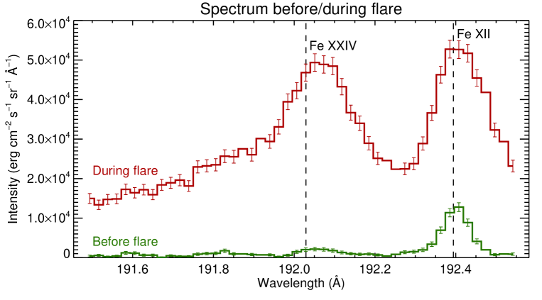
Fig. 2.2: Line profiles of Fe xxiv $192.03$Å and Fe xii $192.39$Å observed by Hinode/EIS on 2011 September 9. Green (Red) profile shows the line profile at the flare site before (during) an M1.2-class flare. Vertical dashed lines indicate the rest wavelengths given by CHIANTI ver. 7 (Dere et al. 1997; Landi et al. 2012).

An example of line profiles is shown in Fig. 2.2. Green (Red) profile shows the line profile at the flare site before (during) an M-class flare on 2011 September 9. In the wavelength range plotted in the figure, there are two strong lines: Fe xxiv $192.03$Å ($\sim 10^{7}\,\mathrm{K}$) and Fe xii $192.39$Å ($\sim 10^{6}\,\mathrm{K}$). Before the onset of the flare, Fe xii $192.39$Å was the only one prominent emission line. During the flare, Fe xxiv $192.03$Å increases in its strength comparable to the neighbor Fe xii $192.39$Å because the high-temperature plasma (up to $\sim 10^{7}\,\mathrm{K}$) is produced by the flare. In addition, the spectrum of Fe xxiv $192.03$Å during the flare shows the shape far different from a single Gaussian profile. It has a long tail in the shorter side in the wavelength direction, which is often referred to as enhanced blue wing (EBW). This line profile is considered to be composed of the rest component and a broadened blueshifted component. As this example shows, line profiles change their shapes depending on cases.

2.1.2 Density diagnostics

Density of the solar corona has been often derived by two methods: EM method and the line ratio method. In EM method, we use the intensity of an emission line. When the assumption that the observed plasma has uniform temperature (i.e., isothermal) along the line of sight, the intensity of an emission line is expressed by

$$I=n_{\mathrm{e}}^{2}\,G(n_{\mathrm{e}},T)\,h\,\text{,}$$ (2.23)

where $n_{\mathrm{e}}$ is electron density ($\mathrm{cm}^{-3}$), $G(n_{\mathrm{e}},T)$ is so-called the contribution function of emission line ($\mathrm{erg}\,\mathrm{cm}^{3}\,\mathrm{s}^{-1}\,\mathrm{sr}^{-1}\,\text{\AA}^{-1}$), and $h$ is the column depth of the observed plasma ($\mathrm{cm}$). Note that the unit of intensity is $\mathrm{erg}\,\mathrm{cm}^{-2}\,\mathrm{s}^{-1}\,\mathrm{sr}^{-1}\,\text{\AA}^{-1}$. The dependence of the contribution function on electron density is usually much weaker than that on temperature, but some emission lines have strong dependence on the electron density, which can be exploited to line ratio method as described after. Using Eq. (2.23), the electron density can be estimated as

$$n_{\mathrm{e}}=\left[\frac{I}{G(n_{\mathrm{e}},T)h}\right]^{1/2}\,\text{,}$$ (2.24)

where the temperature is often assumed to be the formation temperature of the emission line. Practically, it is difficult to know the precise column depth in observation because the 3D morphology of the solar corona cannot be obtained in most cases. One way to determine the column depth $h$ is that we assume the circle cross section of coronal loops or the semi-spherical shape of bright points (small scale loops). Then the column depth is obtained by using the coronal imaging observation. However, the assumption of isothermal plasma is often violated in the solar corona because (1) the overlapping of several structures along the line of sight, and (2) sub-spatial-resolution fine structure of the solar corona. In addition, we obtain only the lower limit of electron density considering that the contribution function is convex upward as a function of temperature.

Second way for the density diagnostics of the solar corona is the line ratio method. We use an emission line pair whose intensity ratio has significant dependence on electron density. If the line ratio is monotonically increases or decreases as a function of the electron density, we can use the line ratio as a tool for the density diagnostics.

The theory about the dependence of intensity on the electron density is described below. An example of the emission line pair Fe xiv $264.78$Å/$274.20$Å is given, both of which involve allowed transitions. The energy levels of Fe xiv and related emissions are shown in Fig. 2.3. In the figure, only transitions having significant influences on the balance of the number of electrons in each level are shown. Numbers in the parenthesis after the characters are the index named for each energy level, which are commonly used in the atomic physics. The transition $10\leftrightarrow 8$ (which produces the emission $\lambda 3143$Å) is omitted because it has negligible contribution on the number equation in this system, considering that almost all of the ions are at the configuration $3s^{2}3p$ (energy level index: $1$ or $2$).

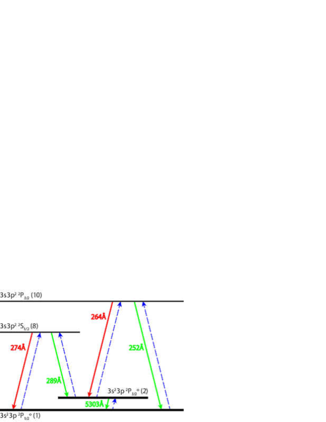
Fig. 2.3: The energy levels and transitions of Fe xiv. Horizontal lines indicate energy levels. The characters beside the lines indicate configurations of the electrons in Fe xiv ion and terms. Numbers in the parenthesis after the characters are the index named for each energy level, which are commonly used in the atomic physics. Full (Dashed) arrows indicate transitions for collisional excitation (emission). Two red arrows are the emission line pair ($8\rightarrow 1$; $\lambda=274.20$Å, $10\rightarrow 2$; $\lambda=264.78$Å) used for density diagnostics in this thesis.

We assume the equilibrium between the numbers of ions in each levels, where the timescales of collisional excitation and radiative decay ($\sim 10^{-9}\,\mathrm{s}$) are much shorter than that of the change of temperature. It almost always holds in the solar corona. Representing the number of ions in the level $i$ by $N_{i}$, the collisional excitation coefficient by $C^{\mathrm{ex}}_{i,j}$ (transition from lower level $i$ to upper level $j$) and the radiative decay by $A_{j,i}$ (transition from upper level $j$ to lower level $i$), the equilibrium between the numbers in each energy level can be written as

$$A_{2,1}N_{2}+A_{8,1}N_{8}+A_{10,1}N_{10} =C^{\mathrm{ex}}_{1,2}N_{1}N_{\mathrm{e}}+C^{\mathrm{ex}}_{1,8}N_{1}N_{\mathrm{e}}+C^{\mathrm{ex}}_{1,10}N_{1}N_{\mathrm{e}}\,\text{,}$$ (2.25)

$$C^{\mathrm{ex}}_{1,2}N_{1}N_{\mathrm{e}}+A_{8,2}N_{8}+A_{10,2}N_{10} =C^{\mathrm{ex}}_{2,8}N_{2}N_{\mathrm{e}}+C^{\mathrm{ex}}_{2,10}N_{2}N_{\mathrm{e}}+A_{2,1}N_{2}\,\text{,}$$ (2.26)

$$C^{\mathrm{ex}}_{1,8}N_{1}N_{\mathrm{e}}+C^{\mathrm{ex}}_{2,8}N_{2}N_{\mathrm{e}} =A_{8,1}N_{8}+A_{8,2}N_{8}\,\text{,}$$ (2.27)

$$C^{\mathrm{ex}}_{1,10}N_{1}N_{\mathrm{e}}+C^{\mathrm{ex}}_{2,10}N_{2}N_{\mathrm{e}} =A_{10,1}N_{10}+A_{10,2}N_{10}\,\text{.}$$ (2.28)

Only three of these equations are independent. If the relative fraction of energy levels as to the ground state would be defined like

$$\alpha_{2}=\frac{N_{2}}{N_{1}}\,\text{,}\,\alpha_{8}=\frac{N_{8}}{N_{1}}\,\text{,}\,\alpha_{10}=\frac{N_{10}}{N_{1}}\,\text{,}$$ (2.29)

Eqs. (2.26)–(2.28) are reduced to

$$\alpha_{2} =\frac{X_{2}}{A_{2,1}+X_{1}N_{\mathrm{e}}}N_{\mathrm{e}}\,\text{,}$$ (2.30)

$$\alpha_{8} =\frac{C^{\mathrm{ex}}_{1,8}+C^{\mathrm{ex}}_{2,8}\alpha_{2}}{A_{8,\mathrm{tot}}}N_{\mathrm{e}}\,\text{,}$$ (2.31)

$$\alpha_{10} =\frac{C^{\mathrm{ex}}_{1,10}+C^{\mathrm{ex}}_{2,10}\alpha_{2}}{A_{10,\mathrm{tot}}}N_{\mathrm{e}}\,\text{,}$$ (2.32)

where

$$A_{8,\mathrm{tot}} =A_{8,1}+A_{8,2}\,\mathrm{s}^{-1}\,\text{,}$$ (2.33)

$$A_{10,\mathrm{tot}} =A_{10,1}+A_{10,2}\,\mathrm{s}^{-1}\,\text{,}$$ (2.34)

$$X_{1} =C^{\mathrm{ex}}_{2,\mathrm{tot}}-\frac{A_{8,2}}{A_{8,\mathrm{tot}}}C^{\mathrm{ex}}_{2,8}-\frac{A_{10,2}}{A_{10,\mathrm{tot}}}C^{\mathrm{ex}}_{2,10}\,\mathrm{cm}^{3}\,\mathrm{s}^{-1}\,\text{,}$$ (2.35)

$$X_{2} =C^{\mathrm{ex}}_{1,2}+\frac{A_{8,2}}{A_{8,\mathrm{tot}}}C^{\mathrm{ex}}_{1,8}+\frac{A_{10,2}}{A_{10,\mathrm{tot}}}C^{\mathrm{ex}}_{1,10}\,\mathrm{cm}^{3}\,\mathrm{s}^{-1}\,\text{,}$$ (2.36)

$$C^{\mathrm{ex}}_{2,\mathrm{tot}} =C^{\mathrm{ex}}_{2,8}+C^{\mathrm{ex}}_{2,10}\,\mathrm{cm}^{3}\,\mathrm{s}^{-1}\,\text{.}$$ (2.37)

The radiance of each emission line ($I_{j,i}$; intensity involving the transition from upper level $j$ to lower level $i$) is represented as

$$I_{j,i}=A_{j,i}N_{j}\,\text{,}$$ (2.38)

therefore, the ratio between two emission lines $264.78$Å (transition: $10\rightarrow 2$)/$274.20$Å (transition: $8\rightarrow 1$) can be calculated as

$$\frac{I_{10,2}(264.78\text{\AA})}{I_{8,1}(274.20\text{\AA})} =\frac{A_{10,2}N_{10}}{A_{8,1}N_{8}}=\frac{A_{10,2}\alpha_{10}}{A_{8,1}\alpha_{8}}$$ (2.39)

$$=\frac{A_{10,2}}{A_{10,\mathrm{tot}}}\frac{A_{8,\mathrm{tot}}}{A_{8,1}}\frac{C^{\mathrm{ex}}_{1,10}+C^{\mathrm{ex}}_{2,10}\alpha_{2}}{C^{\mathrm{ex}}_{1,8}+C^{\mathrm{ex}}_{2,8}\alpha_{2}}$$ (2.40)

$$=\frac{A_{10,2}}{A_{10,\mathrm{tot}}}\frac{A_{8,\mathrm{tot}}}{A_{8,1}}\frac{X_{3}N_{\mathrm{e}}+X_{4}}{X_{5}N_{\mathrm{e}}+X_{6}}\,\text{,}$$ (2.41)

where

$$X_{3} =C^{\mathrm{ex}}_{1,10}X_{1}+C^{\mathrm{ex}}_{2,10}X_{2}\,\mathrm{cm}^{6}\,\mathrm{s}^{-2}\,\text{,}$$ (2.42)

$$X_{4} =C^{\mathrm{ex}}_{1,10}A_{2,1}\,\mathrm{cm}^{3}\,\mathrm{s}^{-2}\,\text{,}$$ (2.43)

$$X_{5} =C^{\mathrm{ex}}_{1,8}X_{1}+C^{\mathrm{ex}}_{2,8}X_{2}\,\mathrm{cm}^{6}\,\mathrm{s}^{-2}\,\text{,}$$ (2.44)

$$X_{6} =C^{\mathrm{ex}}_{1,8}A_{2,1}\,\mathrm{cm}^{3}\,\mathrm{s}^{-2}\,\text{.}$$ (2.45)

Now it is clear that the line ratio Fe xiv $264.78$Å/$274.20$Å has a dependence on electron density in terms of a fractional function. The coefficients $X_{1\text{--}6}$ can be calculated by using the atomic data given by Storey et al. (2000) and Tayal (2008), which is listed in Table 2.1. Calculated coefficients $X_{1-6}$ are tabulated in Table 2.2.

Table 2.1: Transitions involving energy levels $1$, $2$, $8$, and $10$. First column: transitions indicated by indexes of lower and upper level. Second column: wavelength of emission line involving the transition. Third column: collisional excitation coefficients calculated by using effective collision strength in Tayal (2008). The temperature was assumed to be $2\times 10^{6}\,\mathrm{K}$. Fourth column: spontaneous emission coefficients (Einstein’s coefficient $A$) from Storey et al. (2000).

Transition	Wavelength (Å)	$C^{\mathrm{ex}}_{i,j}$ ($\mathrm{cm}^{3}\,\mathrm{s}^{-1}$)	$A_{j,i}$ ($\mathrm{s}^{-1}$)
$1-2$	$5304.49$	$1.55\times 10^{-9}$	$6.023\times 10^{1}$
$1-8$	$274.20$	$2.21\times 10^{-9}$	$1.777\times 10^{10}$
$1-10$	$252.20$	$1.59\times 10^{-9}$	$7.598\times 10^{9}$
$2-8$	$289.15$	$3.70\times 10^{-10}$	$1.147\times 10^{9}$
$2-10$	$264.79$	$8.03\times 10^{-9}$	$3.291\times 10^{10}$

Table 2.2: Values of coefficients $X_{1\text{--}6}$.

$X_{1}$	$1.85\times 10^{-9}$ ($\mathrm{cm}^{3}\,\mathrm{s}^{-1}$)
$X_{2}$	$2.97\times 10^{-9}$ ($\mathrm{cm}^{3}\,\mathrm{s}^{-1}$)
$X_{3}$	$2.68\times 10^{-17}$ ($\mathrm{cm}^{6}\,\mathrm{s}^{-2}$)
$X_{4}$	$9.55\times 10^{-8}$ ($\mathrm{cm}^{3}\,\mathrm{s}^{-2}$)
$X_{5}$	$5.19\times 10^{-18}$ ($\mathrm{cm}^{6}\,\mathrm{s}^{-2}$)
$X_{6}$	$1.33\times 10^{-7}$ ($\mathrm{cm}^{3}\,\mathrm{s}^{-2}$)

The ratio of intensity from two emission lines Fe xiv $264.78$Å/$274.20$Å as a function of electron density is shown in Fig. 2.4.

Fig. 2.4: Line ratio of Fe xiv $264.78$Å/$274.20$Å as a function of electron density calculated by using CHIANTI database. While contribution function of Fe xiv $264.78$Å increases with electron density, that of Fe xiv $274.20$Å decreases with electron density. This makes the line ratio of these two lines behaves monotonically as a function of electron density.

The ratio was calculated by using CHIANTI database version 7 (Dere et al. 1997; Landi et al. 2012). Note that calculating the ratio by using Eq. (2.41) results in slightly larger value than CHIANTI, however, the behavior is fundamentally the same. This discrepancy may come from the difference in the atomic data. In this thesis, we adopt the CHIANTI database because its data is the newest one available at present.

2.2 Instruments

2.2.1 Hinode spacecraft

Hinode (Kosugi et al. 2007) is a Japanese satellite of Institute of Space and Astronomical Science of the Japan Aerospace Exploration Agency (ISAS/JAXA), launched on 2006 September 23 6:36 JST. Hinode has three instruments onboard: the Solar Optical Telescope (SOT), the X-ray Telescope (XRT), the EUV Imaging Spectrometer (EIS). The scientific aims are: (1) to understand the processes of magnetic field generation and transport including the magnetic modulation of the Sun’s luminosity, (2) to investigate the processes responsible for energy transfer from the photosphere up to the chromosphere and the corona, and (3) to determine the mechanisms which induce eruptive phenomena, such as flares and coronal mass ejections (CMEs), and understand these phenomena in the context of the space weather.

The Solar Optical Telescope (SOT) (Tsuneta et al. 2008) consists of the Optical Telescope and the Focal Plane Package (FPP). The SOT consists of a $50$-cm diffraction limit Gregorian telescope, and the FPP includes the narrowband imager (NFI) and the broadband imager (BFI), and the Stokes Spectropolarimeter (SP). The SOT provides unprecedented high spatial and temporal resolution image of the photosphere and the chromosphere by filtergram of NFI/BFI and vector magnetograms calculated through inversion of SP data. The SOT has revealed many kinds of magnetic activity of the Sun such as magnetic flux emergence, submergence, cancellation, and related response of the photosphere and chromosphere.

The X-ray Telescope (XRT) (Golub et al. 2007) has a grazing-incidence optic and a CCD array. Kinds of filters are utilized: entrance aperture prefilters and focal plane analysis filters. The entrance aperture prefilters have two main purposes: (1) to reduce the visible light entering the instrument and (2) to reduce the heat load in the instrument. The focal plane analysis filters have two purposes: (1) to reduce the visible light reaching the focal plane and (2) to provide varying X-ray passbands for plasma temperature diagnostics. The science objectives of the XRT are chromospheric evaporations, reconnection dynamics, polar jets, and coronal holes.

2.2.2 EUV Imaging Spectrometer onboard Hinode

The EUV Imaging Spectrometer (EIS) (Culhane et al. 2007) onboard Hinode observes the solar corona and the upper transition region emission lines in the wavelength range of $170\text{--}210$Å and $250\text{--}290$Å. The emission line centroid position and the emission line width allow us to know the Doppler velocity and the nonthermal velocity of the observed plasma. The plasma temperature and density can be measured by using the intensity ratio of temperature or density sensitive line pair (detail was given in Section 2.1.2). The science aims of EIS is to investigate the coronal/photospheric velocity field comparison in active regions and understand the dynamics of flares (e.g., by coordination with SOT), and to detect the heating signatures in the corona.

Previous spectrometers designed to operate in the wavelength range of $50\text{--}500$Å have employed grazing incidence optical systems, since the normal incidence reflectivity within this wavelength range is quite small for the usual optical materials. The microchannel plate array detectors are commonly used, which provide high spatial resolution, however, they have low quantum efficiencies ($\mathrm{QE}\leq 20$%). EIS adopted normal incidence operation through the use of multilayer coatings applied to both mirror and gratings. Furthermore, the use of thinned back-illuminated CCDs to register the diffracted photons make QE values be $2\text{--}3$ times larger than those for micro channel plate systems. EIS has a large effective area in two EUV wavelength ranges, $170\text{--}210$Å and $250\text{--}290$Å. The optical design of EIS is displayed in Fig. 2.5.

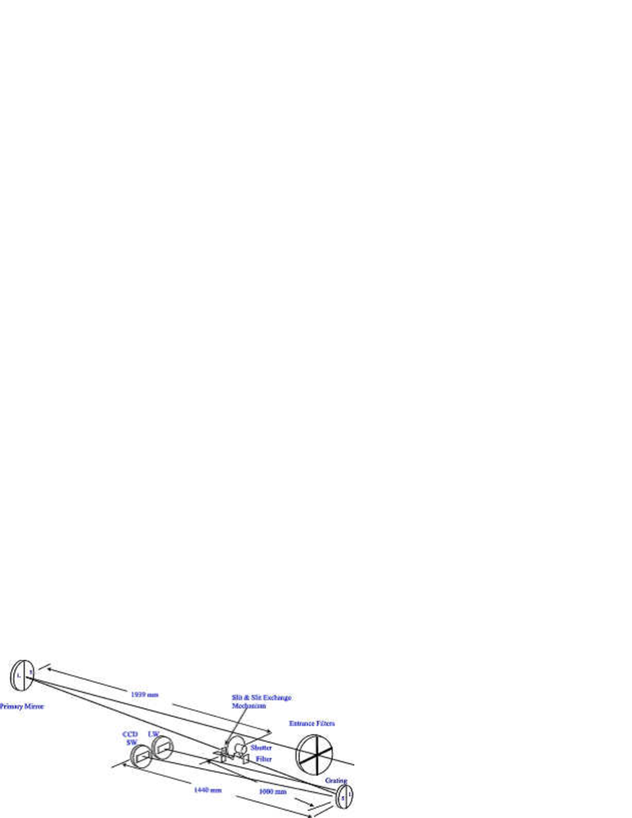
Fig. 2.5: Mechanical design of the EUV Imaging Spectrometer (EIS) onboard Hinode. Excerpted from Culhane et al. (2007).

The solar radiation enters EIS through a thin $1500$Å Al filter which interrupts the transmission of visible radiation (i.e., the brightest wavelength range in the solar spectrum). Incident photons are focused by the primary mirror onto a slit/slot and then on a toroidal concave grating. Two differently optimized Mo/Si multilayer coatings are used to matching halves of both mirror and grating. Then, diffracted photons are registered by a pair of thinned back-illuminated CCDs. Exposure times are controlled by a rotating shutter. Two spectroscopic slits ($1^{\prime\prime}$ and $2^{\prime\prime}$) and two spectroscopic imaging slots ($40^{\prime\prime}$ and $266^{\prime\prime}$) are used in a slit exchange mechanism, which allows the selection of four different apertures corresponding to each scientific purpose. Raster scan observations are made by a piezoelectric drive system which rotates the primary mirror. A raster scan has a field of view of $600^{\prime\prime}$ in the dispersion direction (the east-west direction on the solar surface) and $512^{\prime\prime}$ in the slit height direction (the north-south direction on the solar surface). There is a coarse mechanism that can offset the mirror by $\pm 15^{\prime}$ from the spacecraft pointing in the east-west direction. The overall instrumental properties are given in Table 2.3.

Table 2.3: EIS properties (Korendyke et al. 2006; Culhane et al. 2007).

Wavelength bands	$170\text{--}210$Å and $250\text{--}290$Å
Peak effective areas	$0.30\,\mathrm{cm}^{2}$ and $0.11\,\mathrm{cm}^{2}$
Primary mirror	$15\,\mathrm{cm}$ diameter; two Mo/Si multilayer coatings
Grating	Toroidal/laminar, $4200\,\mathrm{lines\,mm^{-1}}$, two Mo/Si multilayers
CCD cameras	Two back-thinned e2v CCDs, $2048\times 1024\times 13.5\,\mathrm{\mu\,m\,pixels}$
Plate scales	$13.53\,\mathrm{\mu\,m\,arcsec^{-1}}$ (at CCD); $9.40\,\mathrm{\mu\,m\,arcsec^{-1}}$ (at slit)
Spatial resolution	$\sim 2^{\prime\prime}$
Field of view	$600^{\prime\prime}\times 512^{\prime\prime}$, offset center: $\pm 825^{\prime\prime}$ in E-W direction
Raster	$1^{\prime\prime}$ in $0.7\,\mathrm{s}$ (Minimum step size: $0^{\prime\prime}.123$)
Slit/slot widths	$1^{\prime\prime}$, $2^{\prime\prime}$ (slit), $40^{\prime\prime}$ and $266^{\prime\prime}$ (slot)
Instrumental broadening	$\sim 2.5\,\mathrm{pixels}$
Spectral resolution	$47\,\mathrm{m}$Å (FWHM) at $185$Å; $1\,\mathrm{pixel}=22\,\mathrm{m}$Å or
	approx. $25\,\mathrm{km\,s^{-1}}$
Temperature coverage	$\log T=4.7,\,5.6,\,5.8,\,5.9,\,6.0\text{--}7.3$
CCD frame read time	$0.8\,\mathrm{s}$
Line observations	Simultaneous observation of up to $25$ lines

EIS carries out observations in two modes: raster scan mode and sit-and-stare mode. In raster scan mode, the slit/slot scans the objective region on the solar surface. The obtained data will be three dimensional ($x,y$, and wavelength), which is suitable for studying spatial variation of the spectra. In the sit-and-stare mode, the slit/slot is fixed at a target position on the solar surface and is tracking the target by compensating for the solar rotation during the observation. The data obtained in the sit-and-stare mode provide the temporal variability of the spectra, which is suitable for investigating phenomena like oscillations, jets, or microflares.

Chapter 3 Average Doppler shifts of the quiet region

3.1 Introduction

Measurement of the Doppler shift of an emission line is an important method to investigate the velocity of a target in astrophysics. EIS onboard Hinode aims to measure a Doppler shift with an accuracy in the order of $10^{-3}$Å which corresponds to several $\mathrm{km}\,\mathrm{s}^{-1}$ in the EUV wavelength range. The flow speed in the corona is typically the order of $\mathrm{km}\,\mathrm{s}^{-1}$ in the quiet region and up to several tens of $\mathrm{km}\,\mathrm{s}^{-1}$ in active regions. The method is simple in the sense that we measure a line centroid and calculate the difference from the rest wavelength known in advance, however, the practical analysis is far more complex.

Since EIS does not have the absolute calibration mechanism for wavelength, we often refer the average line centroid of the quiet region included in the field of view as zero. This is based on the idea that the quiet region has smaller velocity than that of active regions. The Doppler velocity derived through this procedure should be actually regarded as just a difference of the Doppler shift from that of the quiet region. At present, the Doppler velocities of coronal emission lines in the quiet region have not been investigated with an precision better than $\simeq 10\,\mathrm{km}\,\mathrm{s}^{-1}$, considering the several uncertainties described below. We need another way to deduce the Doppler velocity in the quiet region different from previous data analysis in the literature. For the precise measurements of the Doppler shift, we need to take care of several points below.

First point is a lack of our knowledge about precise rest wavelengths of some emission lines. The database of emission lines provided by NIST shows that the rest wavelengths are determined in the order of $10^{-3}$Å in most cases. We actually sometimes observe an emission line in different wavelength predicted by the theoretical calculation. This means that it is not possible to measure the Doppler shift more accurately than that deviation even if we can obtain the precise line centroid with small statistical error by long exposure time in an observation.

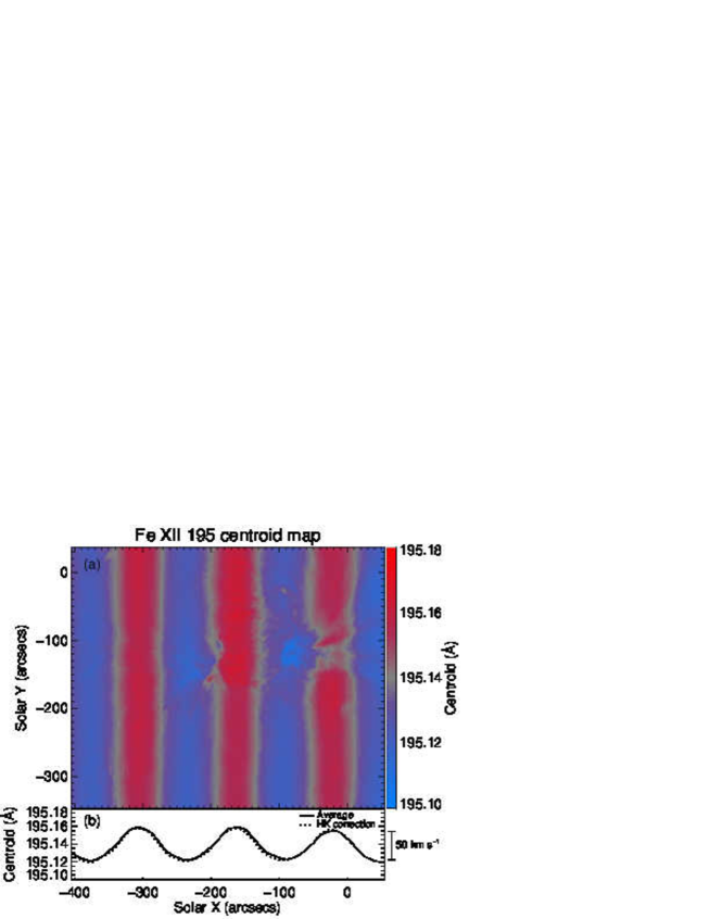
Fig. 3.1: (a) Doppler shift map without any wavelength corrections for orbital variation. Only the spectrum tilt was removed by using the SSW package. (b) The line centroid averaged in $y$ direction (solid) and the orbital variation estimated by Kamio et al. (2010)’s model (dotted). Note that the dotted curve was shifted so that it has the same value as the solid curve at the left edge of the FOV ($x=-405^{\prime\prime}$).

Second point is the drift of the spectrum signals on the CCDs which mainly comes from the displacement of the grating component in accordance with the thermal environment of the EIS instrument (Brown et al. 2007). The Hinode spacecraft flies in the Sun synchronous orbit and the angle of which the spacecraft faces to the Earth changes periodically in $\simeq 98\,\mathrm{min}$. The temperatures of the components in the EIS instrument change due to the variation of the Earth radiation with that period. This causes the quasi-periodic drift of the spectrum of $\sim 0.05$Å which corresponds to $50$–$75\,\mathrm{km}\,\mathrm{s}^{-1}$ at wavelength of $200$–$300$Å. Fig. 3.1 shows an example of this effect. The displacement of the spectrum is obviously larger than the variation in the solar corona, therefore it becomes much important to remove the instrumental effect before the measurement of the Doppler shift. Although the temperature changes in the components of EIS are roughly periodic, the calibration is never simple because the temporal behavior also changes with the seasonal variation of the orbit of the spacecraft, and there are also phase difference in the temperature variation in each component. The package developed by Kamio et al. (2010) has been widely used to correct the wavelength scale which varies in accordance with the temperature of the instrument. They modeled the orbital variation of the wavelength scale by a linear relationship with the temperatures of components in the EIS instrument and some other parameters (e.g., pointing coordinates). The developed model basically reproduces the observed spectrum drift, but there are residuals of $4$–$5\,\mathrm{km}\,\mathrm{s}^{-1}$ in the standard deviation from the observed data.

Third point is that the model above assumes that the Doppler shift of Fe xii $195.12$Å averaged in each exposure equals zero, which may not be the actual case precisely. The SUMER observations revealed that an emission line Ne viii $770$Å ($\log T\,[\mathrm{K}]=5.8$) are blueshifted at the disk center corresponding to the Doppler velocity of $-2$ – $-3\,\mathrm{km}\,\mathrm{s}^{-1}$ in the quiet region (Peter 1999; Teriaca et al. 1999). The Doppler shift of Fe xii $1242$Å was measured by Teriaca et al. (1999), which reported that the emission line is blueshifted by $-10\,\mathrm{km}\,\mathrm{s}^{-1}$ in an active region (Teriaca et al. 1999). That Fe xii emission line was too weak for the measurement in the quiet region, and we cannot exclude the possibility that emission lines in the coronal temperature are shifted from the rest wavelength in the quiet region. Although the model of Kamio et al. (2010) is an useful tool to compensate the orbital variation of the wavelength scale and it is now included in the standard EIS software in SSW, taking into account all three factors described above, we can not discuss the Doppler velocity smaller than $\sim 5\,\mathrm{km}\,\mathrm{s}^{-1}$ by using only their model.

In this chapter, we exploited the data which covers the meridional line of the Sun in order to deduce the Doppler shifts at the center of the solar disk compared to those at the solar limb where the Doppler velocities are considered to be the best zero point at present. Such observations enable us to study the center-to-limb variation of the Doppler shift of emission lines, which solve the first point in the measurement of the Doppler shift described above (i.e., a lack of the knowledge about the precise rest wavelength). This analysis is based on the idea that the corona flows statistically in the radial direction from the global view. We analyzed the spectra by integrating with a spatial scale of $50^{\prime\prime}$ in order to compensate the non-radial motions in a statistical sense.

Since there are only few coronal emission lines in the spectra obtained by SUMER and its predecessors with strength enough for their line centroids to be measured in the quiet region, previous observations could only measure the center-to-limb variation of the transition region lines (Roussel-Dupré & Shine 1982; Peter 1999) whose formation temperature was $\log T\,[\mathrm{K}]\leq 5.8$. Our analysis challenges the center-to-limb variation of the Doppler shifts of several coronal emission lines ($\log T\,[\mathrm{K}]\geq 6.0$), and determine the average Doppler shifts in the quiet region at the disk center. The results in this chapter will be used as a reference of Doppler velocities for the analysis of the outflow in an active region (Chapter 4).

3.2 Observations

Based on the idea that emission lines are not shifted at the limb because our line of sight passes symmetrically the solar corona (Peter 1999), we can set the Doppler velocity at the limb as zero then derive the Doppler velocities at the disk center. In order to investigate the center-to-limb variation of the Doppler shifts and measure those at the disk center, we exploited data taken during the coordinated observations between three instruments onboard Hinode (usually referred to as Hinode Observing Plan 79; hereafter we use the term HOP79). While these observations were originally intended to investigate the variation of solar irradiance along the 11-year solar cycle mainly by SOT observations, EIS is requested to take spectra with long exposures. During the observations, the pointings of the satellite are gradually moved from the south pole to the north pole (north–south scan), or from the east limb to the west limb (east–west scan), so that the data cover the solar surface from one limb to the other limb.

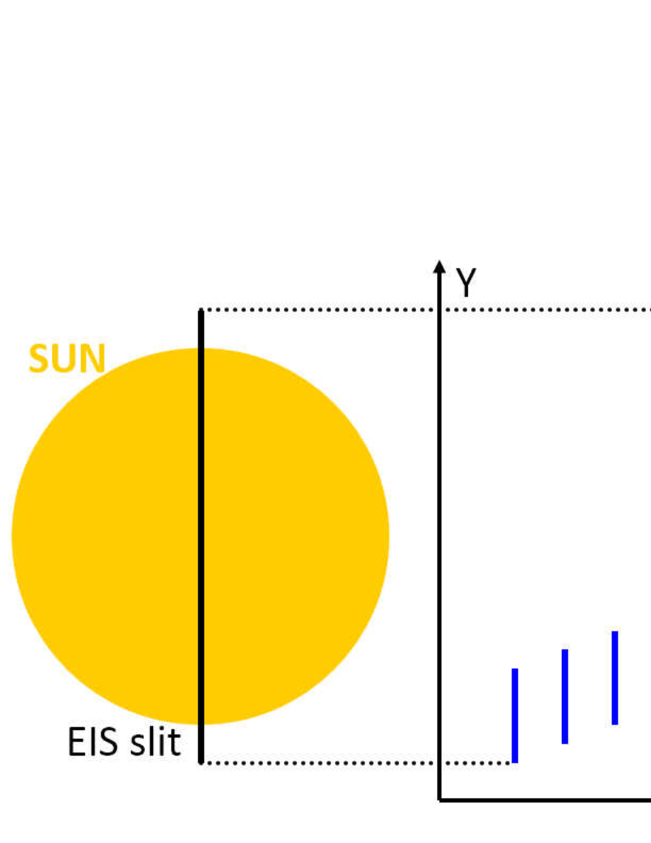
Fig. 3.2: Schematic picture of the north–south scan in HOP79.

In this analysis, we used the north–south scans which obtain the solar spectra without spatial gap between pointing changes (i.e., overlapping FOVs in each pointing by $300^{\prime\prime}$). The schematic picture of the scan is shown in Fig. 3.2. This observation enables us to investigate the center-to-limb variation of Doppler shifts of emission lines by aligning the line centroids between the overlapping locations. Note that in the east–west scans, EIS FOVs do not overlap with each pointing so that it is not possible to investigate the center-to-limb variation of the Doppler shifts. Thus, we concentrate on the north–south scans in this analysis here.

In the observations, $1^{\prime\prime}$ slit was used and the FOV in each pointing was $5^{\prime\prime}\times 512^{\prime\prime}$ (i.e., five exposures at each pointing). The exposure time was $120\,\mathrm{s}$, which is enough to obtain good signal-to-noise (S/N) ratio for many coronal emission lines even in the quiet region. The EIS usually records the spectra with a finite width in the wavelength direction (called as spectral window). The EIS study analyzed here consists of 16 spectral windows with the spectral widths of $24$–$48$ pixels ($\simeq 0.5$–$1.0$Å), which were wide enough to include whole of emission lines (cf. typical Gaussian width of emission lines in the quiet region does not exceed $\simeq 0.05$Å).

Some recent studies have challenged the precise measurement of Doppler velocities of coronal structures by referring the centroids of emission lines determined from EIS spectra at the limb (Warren et al. 2011; Young et al. 2012; Dadashi et al. 2012), however, there is a remaining factor for the uncertainty in the measurement. They all used a calibration of wavelength developed by Kamio et al. (2010) when comparing the centroids measured at the limb with those measured at their target coronal structures. Therefore, their results are thought to have the error of $\simeq 5\,\mathrm{km}\,\mathrm{s}^{-1}$. The analysis here is free from that problem with overlapped scans from the south limb to the north limb, and will help us to determine the Doppler velocities with much carefulness.

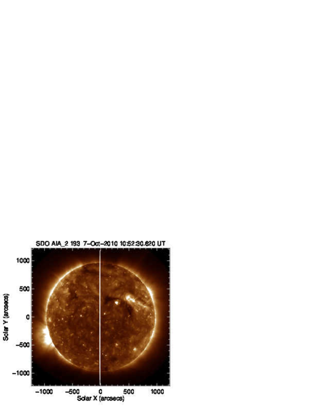
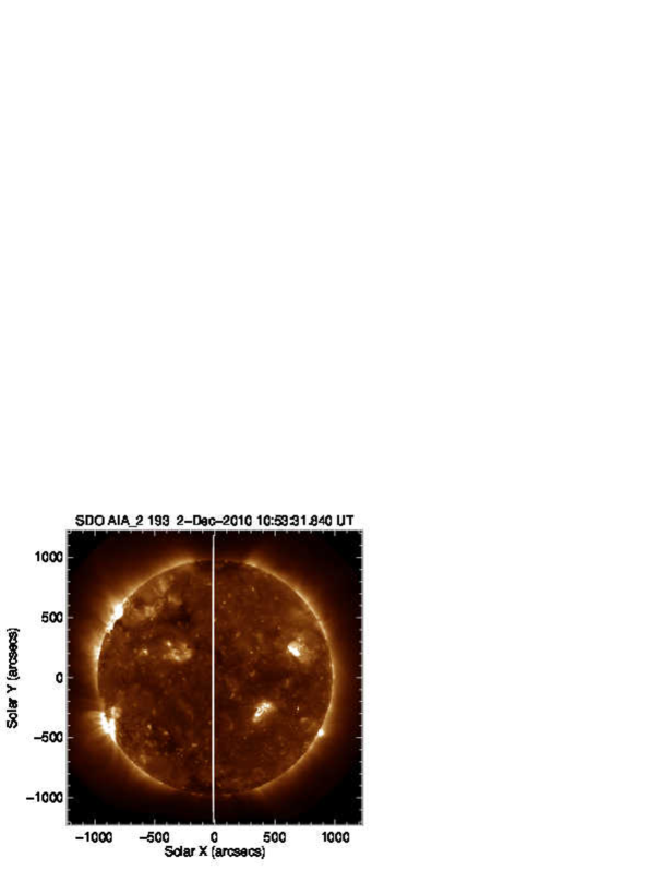
Fig. 3.3: SDO/AIA $193$Å passband images at the start of each HOP79. Upper: October. Lower: December. A white vertical line in each image indicates the location where EIS took spectral data.

The analyzed HOP79 data were taken during 2010 close to the bottom of the solar cycle in order to avoid the influence of active regions with relatively larger systematic flows than the quiet region. When a spectral scan of EIS includes some active regions, there are several possibilities which cause the Doppler shift of an emission line. Firstly, there can be seen many active phenomena like microflares, which induce plasma flows up to several ten $\mathrm{km}\,\mathrm{s}^{-1}$ in the corona. Secondly, the corona in active regions generally has higher electron density ($10^{9-10}\,\mathrm{cm}^{-3}$; not flare condition) than in the quiet region ($10^{8-9}\,\mathrm{cm}^{-3}$), which often produces a fake shift of an emission line when another emission line exists in the neighbor whose emissivity strongly depends on the electron density. Obviously, this is not the indication of the real flow. Thirdly, a persistent upflow up to several tens of $\mathrm{km}\,\mathrm{s}^{-1}$ is often observed at the edge of active regions (Doschek et al. 2008; Harra et al. 2008) which causes the blueshift of coronal emission lines.

Many of the data taken in HOP79 after 2011 include active region(s) and its remnant in high latitude, and since the presence of active regions in spectral scan may affect our analysis, we analyzed the spectral data during 2010. The data including a large coronal hole or active region(s) were not used in this analysis: January, February, March, May, July, August, September, and November. In the analysis below, we concentrated the data in October and December. The context images taken by SDO/AIA are shown in Fig. 3.3. A white vertical line in each image indicates the location where EIS took spectral data.

3.3 Data reduction and analysis

In this section, the procedure of analysis is described. First, we look over line profiles in order to check whether the single-Gaussian fitting is suitable for each emission line or not. Emission lines within the EUV range observed with EIS are often blended by neighboring ones, and this effect might cause a fake shift of the target emission line.

3.3.1 Line profiles

Fig. 3.4: Intensity (ordinate) as a function of the solar $Y$ (abscissa). A number in the left upper corner in each panel is the logarithmic formation temperature for the emission line. A Vertical dashed line indicates the limb location determined from the Fe viii intensity. Horizontal bars at the bottom in each panel shows the location where the spectrum was averaged and shown in Fig. 3.5.

Fig. 3.4: Continued.

In order to decide emission lines to be analyzed, we first started from looking line profiles taken by EIS. Fig. 3.4 shows the spatial distribution of intensities near the south limb during HOP79 in 2010 October 7–8. The intensities shown here are calculated by integrating over each spectral window. Panels in the figure are in the order of the formation temperature. The vertical dashed line at $y=-960^{\prime\prime}$ in each panel indicates the limb location which was determined from the maximum point of Fe viii intensity since the limb was clearly seen in the transition region lines (O iv–v, Fe viii and Si vii) due to the well-known “limb brightening” effect which arises from the fact that the solar corona is optically thin. In that situation, when we move our line of sight from the solar disk inside the limb to above the limb, the length of our line of sight becomes twice because there are no occulting structures above the limb. For coronal lines from Fe x–xii, the intensity is stronger inside the limb than that off the limb, while for coronal lines like Fe xiii and Fe xv the intensity is stronger outside the limb compared to the disk (i.e., inside the limb).

Line profiles on the solar disk ($y=-750^{\prime\prime}$; solid line) and above the limb ($y=-1050^{\prime\prime}$; dashed line) for all spectral windows taken by EIS during HOP79 on 2010 October 7–8 are shown in Fig. 3.5. Panels are in the order of the formation temperature as same as in Fig. 3.4. The line profiles were integrated and averaged by the span of $100^{\prime\prime}$ in the $y$ direction and the integrated ranges are indicated by horizontal bar in Fig. 3.4. We note characteristics of the emission lines seen in each spectral window below.

Fig. 3.5: Line profiles on the disk (solid) and off the limb (dotted). A number in the left upper corner in each panel is the logarithmic formation temperature for the emission line. Error bars include photon noise and uncertainty in CCD pedestal and dark current.

Fig. 3.5: Continued.

3.3.1.1 The transition lines

He ii

He ii $256.32$Å is known to be one of the strongest emission lines in EIS spectra and the only one with the formation temperature below $\log T\,[\mathrm{K}]=5.0$. The emission is very weak above the limb which indicates that it comes from the bottom of the corona or lower. As seen in the solid line profile, He ii $256.32$Å has a long enhanced red wing. This is the contribution from Si x $256.37$Å, and this blend makes the analysis of He ii $256.32$Å much complex. Ideally, we can remove this Si x by referring Si x $261.04$Å since these line pair has constant intensity ratio of $I_{256.37}/I_{261.04}=1.25$ (CHIANTI ver. 7; Landi et al. 2012) because their upper level of the transition are the same. The intensity ratio might be possibly measured above the limb where He ii becomes much more weaker than inside the solar disk. However, as seen from the off-limb spectrum (dotted histogram) of Si x $261.04$Å in Fig. 3.5, it was not strong enough to be used as a reference emission line (i.e., noisy). Therefore, we did not use He ii $256.32$Å in this analysis.

O iv–v

The EIS data analyzed here includes two oxygen emission lines: O iv $279.93$Å ($\log T\,[\mathrm{K}]=5.2$) and O v $248.48$Å ($\log T\,[\mathrm{K}]=5.4$). Previous observations have reported that the transition region lines around $\log T\,[\mathrm{K}]\simeq 5.0$–$5.5$ are redshifted by up to $\sim 10\,\mathrm{km}\,\mathrm{s}^{-1}$ at the disk center (Chae et al. 1998; Peter & Judge 1999; Teriaca et al. 1999), and that it is meaningful to analyze those oxygen lines to confirm the consistency between the previous observations and our results. Since the spectra of these emission lines are much weaker compared to other emission lines observed (e.g., Fe emission lines), we integrated the spectra almost all along the slit ($500^{\prime\prime}$) at the expense of spatial resolution in the analysis as described in Section 3.B. As seen from the spectra in Fig. 3.5, the integration of $100$ pixels obviously does not look enough to measure the precise line centroid.

Fe viii and Si vii

Two emission lines Fe viii $186.60$Å and Si vii $275.35$Å are strong and well-isolated from other strong ones, in addition, the formation temperatures are similar. There is a Ca xiv emission line near the line centroid of Fe viii $186.60$Å, but its influence is thought to be very weak in the quiet region due to its high formation temperature of Ca xiv ($\log T\,[\mathrm{K}]=6.7$). Mg vi $268.99$Å has formation temperature similar to that of Fe viii and Si vii, but it was too noisy to achieve the precision of several $\mathrm{km}\,\mathrm{s}^{-1}$ so we did not use this line.

3.3.1.2 Coronal lines

Fe ix

At the longer wavelength side in the spectral window of Fe xi $188.21$Å/$188.30$Å, there is a Fe ix $188.49$Å, which is isolated and relatively strong. We can fill the wide temperature gap between Fe viii ($\log T\,[\mathrm{K}]=5.69$) and Fe x ($\log T\,[\mathrm{K}]=6.04$) by using this line.

Fe x

There are two emission lines from Fe x: $184.54$Å/$257.26$Å in the analyzed EIS data. Both are free from any significant blend by other lines near the line center. Note that at the red wing of Fe x $184.54$Å, a weak line Fe xi $184.41$Å exists. But this line is much weaker than Fe x $184.54$Å in the quiet region.

Fe xi

For Fe xi emission lines, there are three spectral windows including them: $180.40$Å, $188.21$Å, and $192.81$Å. All these three lines unfortunately suffer from a significant blending. Near the line center of Fe xi $180.40$Å, there is Fe x $180.44$Å ($\sim 2$ pixels apart each other in the EIS CCD). This emission line is density sensitive and becomes stronger at a location where the electron density is higher. This may cause a systematic redshift compared to the result from other Fe xi emission lines. As seen in the Fe xi $188.21$ spectrum in Fig. 3.5, two emission lines with comparative strength are blending each other: Fe xi $188.21$Å/$188.30$Å. We fitted Fe xi $188.21$Å/$188.30$Å by double Gaussians, which is considered to be robust because these two emission lines are both strong and their line profiles usually have two distinct peaks. The third emission line Fe xi $192.81$Å is significantly blended by the transition region lines O v $192.90$Å in the quiet region, so we did not use that line.

Fe xii

Two emission lines Fe xii $192.39$Å and $195.12$Å are both strong and suitable for the analysis of the quiet region. One problem in the analysis of Fe xii $195.12$Å is that there exists a blend by Fe xii $195.18$Å and the line ratio $195.18$Å/$195.12$Å has a sensitivity for the electron density. This will cause an apparent shift of the emission line toward the longer wavelength (i.e., redshift) especially in active regions and at bright points where the electron density typically becomes higher by an order of magnitude than that in the quiet region.

Fe xiii

Fe xiii $202.04$Å is only one strong emission line from Fe xiii in this EIS study and known to be a clean line without any significant blend. Different from emission lines with lower formation temperature, the spectra of Fe xiii $202.04$Å above the limb and inside the solar disk shown in Fig. 3.5 indicate that the off-limb spectrum is stronger than the disk spectrum by approximately twice. This value is what can be expected from the limb brightening effect.

Fe xiv–xv

Emission lines Fe xiv $264.78$Å and Fe xv $284.16$Å were very weak in the quiet region even with the exposure time of $120\,\mathrm{s}$. The off-limb spectrum and the disk spectrum of Fe xv indicate the same behavior as those of Fe xiii. However, the spectra of Fe xiv behave differently from them. This is considered to be the influence of an emission line Fe xi $264.77$Å existing near the line centroid of Fe xiv. In the quiet region, contribution from Fe xi could become relatively strong compared to Fe xiv because the average temperature is slightly lower than that in active regions. It is possible that Fe xv has the similar problem in the quiet region. Therefore, we did not analyze Fe xiv and Fe xv emission lines here in order not to derive improper results.

3.3.2 Fitting

Fig. 3.6: Line profile at the disk center taken during HOP79 in 2010 October. (a) Fe xi $188.21$Å/$188.30$Å, and (b) Fe xiii $202.04$Å. Error bars include photon noise and uncertainty in CCD pedestal and dark current.

Most of the emission lines used in this analysis can be considered to be well fitted by a single Gaussian because they are isolated and strong. In order to reduce the fluctuations caused by the existence of coronal structures (e.g., bright points) and non-radial motions, we spatially integrated the spectra by $50^{\prime\prime}$ in the $y$ direction. One example of fitting Fe xiii $202.04$Å by a single Gaussian is shown in panel (a) of Fig. 3.6. Upper part of the panel shows the line profile at the disk center taken during HOP79 in 2010 October and a green line is a fitted single Gaussian. We used a single Gaussian in the form of

$$f(\lambda)=a_{0}\exp\left[-\dfrac{\left(\lambda-a_{1}\right)^{2}}{2a_{2}^{2}}\right]+a_{3}\,\mathrm{.}$$ (3.1)

Coefficients $a_{i}$ ($i=0,1,2,3$) respectively represent peak, line centroid, line width (Gaussian width), and constant background. Lower part shows residuals from the fitted Gaussian, which do not exceed $\sim 2$% of the peak in the spectrum and are comparative to the errors. Only the wavelength range used for the fitting is plotted in the lower panel. The single Gaussian fitting was applied to the emission lines Fe viii $186.60$Å, Si vii $275.35$Å, Fe ix $188.49$Å, Fe x $184.54$Å/$257.26$Å, Fe xi $180.40$Å, Fe xii $192.39$Å/$195.18$Å, and Fe xiii $202.04$Å. Each spectra were fitted by using $8$–$14$ pixels which include each emission line.

As an exception, Fe xi $188.21$Å and $188.30$Å were fitted by double Gaussians because they clearly overlap with each wing. In this case we used double Gaussians with constant background. Upper part of panel (b) shows a line profile of the Fe xi emission lines at the disk center as same as Fe xiii $202.04$Å, and a green line indicates the result of fitting.

In order to check the robustness of our double Gaussian fitting for Fe xi $188.21$Å/$188.30$Å, the scatter plot for fitted line centroids of two emission lines is made as shown in panel (a) of Fig. 3.7. Theoretically, the line centroids from the same ion have the relationship $\lambda_{2}/\lambda_{1}=\mathrm{const.}$ ($\lambda_{1}$ and $\lambda_{2}$ are the line centroid of two emission lines) considering the Doppler effect cancels out because the factor $1+v/c$ is common between the emission lines from the same ion. The two line centroids clearly have the positive correlation with the correlation coefficient of $R=0.973$. In addition, the ratio of two line centroids was $\lambda_{188.30}/\lambda_{188.21}=1.0004487\pm 2.9\times 10^{-6}$ in the average as shown in panel (b), which is almost identical to the theoretical value ($1.0004405$). Thus, we conclude that the double Gaussian is reliable.

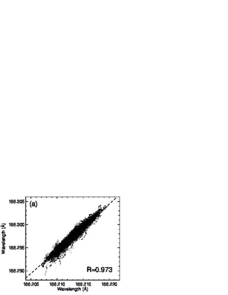
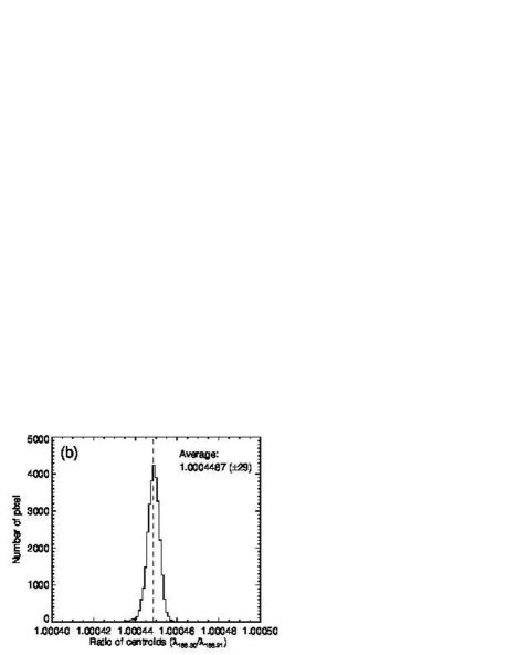
Fig. 3.7: (a) Scatter plot for line centroids of Fe xi $188.21$Å/$188.30$Å. Dashed line indicates a regression line based on a model function $y=ax$. The coefficient $a$ was $1.0004487(\pm 1\times 10^{-7})$. The correlation coefficient was $R=0.973$. (b) Histogram for the ratio of line centroids ($\lambda_{188.30}/\lambda_{188.21}$). The average value was $1.0004487$ and the standard deviation was $2.9\times 10^{-6}$.

3.3.3 Calibration of the spectrum tilt

The spectra taken by EIS are known to be slightly tilted from $y$ axis when projected onto the CCDs (hereafter we call this effect as the spectrum tilt). This arises from the subtle misalignment of the spectroscopic slits, the grating component and the CCDs. The tilts of the slits and the grating component should cause the same degree of the tilts in the observed spectra. The two CCDs are known to be displaced a little each other, which makes the spectrum of the two CCDs different. The spectrum tilt is crudely $1$ pixel in the wavelength direction along the full height of the CCDs ($1024$ pixels), which corresponds to $\simeq 20$–$30\,\mathrm{km}\,\mathrm{s}^{-1}$.

The current standard EIS software calibrates this effect by referring the spectrum tilt obtained at the off limb. It is fixed and has no dependence on wavelength. However, the spectrum tilt may have different characteristics on the two CCDs and even with wavelength. Since we aim to deduce Doppler velocities in the order of a few $\mathrm{km}\,\mathrm{s}^{-1}$, we carefully investigated the spectrum tilt by analyzing the scan taken in the quiet region at the solar disk as described in Section 3.A. The obtained tilts were used to calibrate the north–south scan data from HOP79.

3.3.4 Alignment of data between exposures

Fig. 3.8: Left: line centroids of Fe xiii $202.04$Å during the north–south scans derived through the standard EIS analysis software provided by the SSW package. Different colors respectively indicate data points obtained at each pointing of the satellite ($20$ locations from the south pole to the north pole). Right: line centroids aligned between neighboring pointings. Data arrays were shifted in vertical axis of the panel so that the difference of line centroids between overlapping region becomes smallest.

The analysis in this chapter requires carefulness by the order of $1\,\mathrm{km}\,\mathrm{s}^{-1}$, which means we need a little more finer reduction than the procedures provided by the standard EIS software in the SSW package. The current SSW package includes a robust wavelength calibration developed by Kamio et al. (2010), but there remains an uncertainty of $\lesssim 10\,\mathrm{km}\,\mathrm{s}^{-1}$ due to two reasons described in Section 3.1. In order to reduce this uncertainty, we (1) aligned five exposures in one pointing, and (2) aligned them between the neighboring pointings so that the sum of squared difference in overlapped region becomes smallest. Here we assumed that the average Doppler shift in the quiet region is independent of time. An example of alignment is shown in Fig. 3.8. In order to compare our reduction to the standard package, the line centroid calibrated by SSW is plotted in panel (a). The data after aligned are shown in panel (b), which is much less dispersed than the data in panel (a). From this result, we confirmed that the fluctuation up to $0.005$Å ($\simeq 7\,\mathrm{km}\,\mathrm{s}^{-1}$) is still remained after analyzed through the standard SSW package.

Note that a systematic linear behavior remains for some emission lines even after those careful analysis above. This may come from the residual of the spectrum tilt removal, but we do not specify the exact reason at present. In order to compensate the linear component appropriately as long as possible, we adopted the idea that the Doppler shifts must be symmetric about the disk center, which should be safe in the global FOV.

3.4 Center-to-limb variation

Fig. 3.9: Center-to-limb variations of emission line centroid obtained from the north–south scan during HOP79 in 2010 October. Each panel shows the variation of different emission line: (a) Fe viii $186.60$Å, (b) Fe x $184.54$Å, (c) Fe xi $188.21$Å, (d) Fe xii $192.39$Å, and (e) Fe xiii $202.04$Å. Two vertical dotted line indicate that the data were fitted between those. Dashed lines are the fitted line which has a form of $v(y)=v_{0}\cos\theta$ ($y=R_{\odot}\sin\theta$).

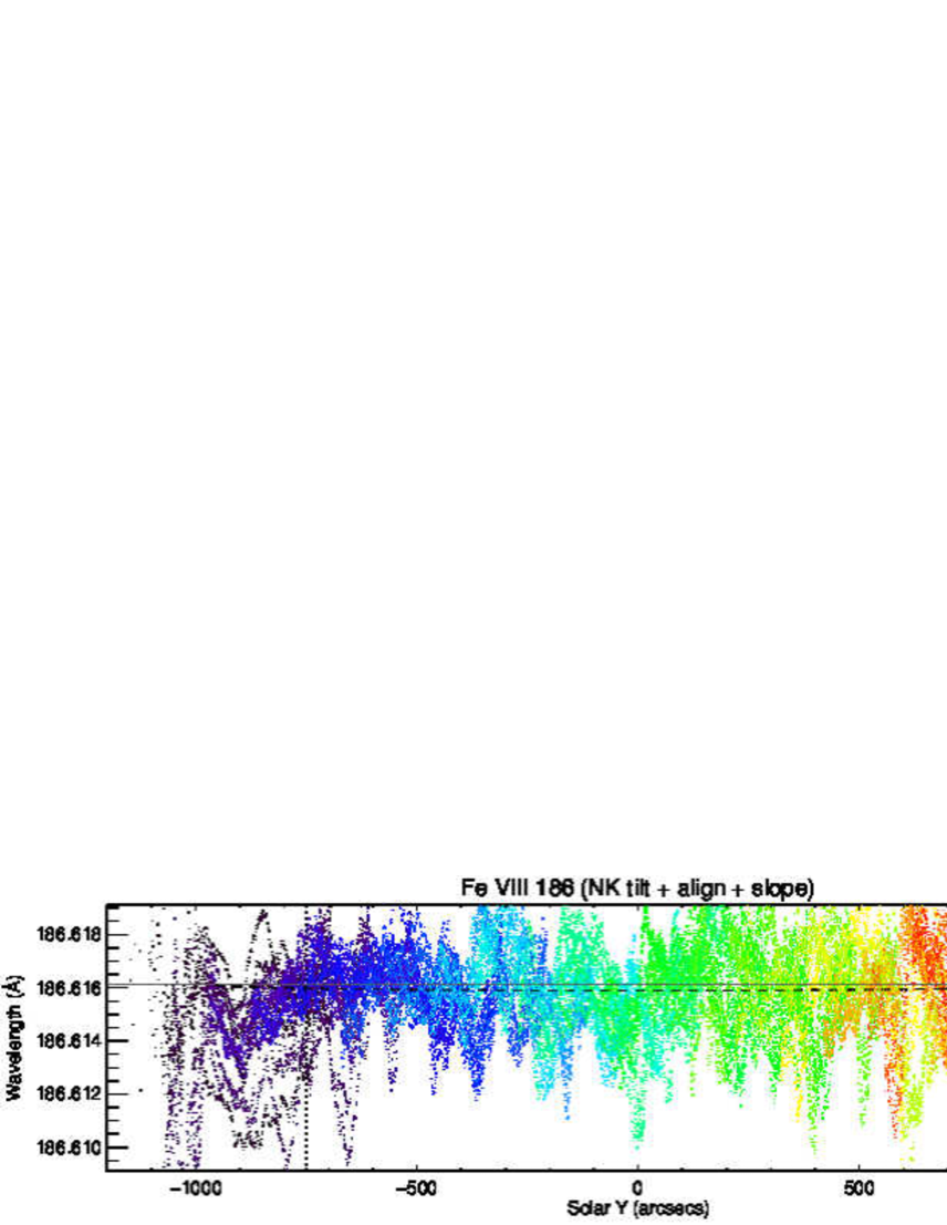
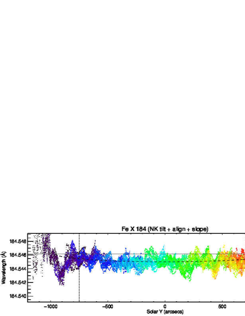
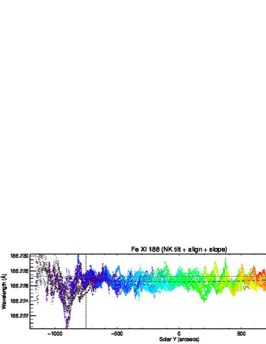
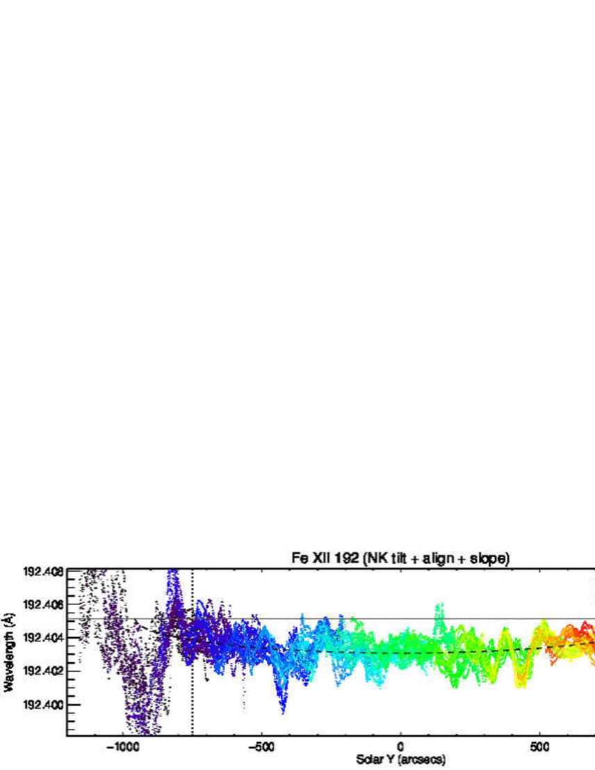
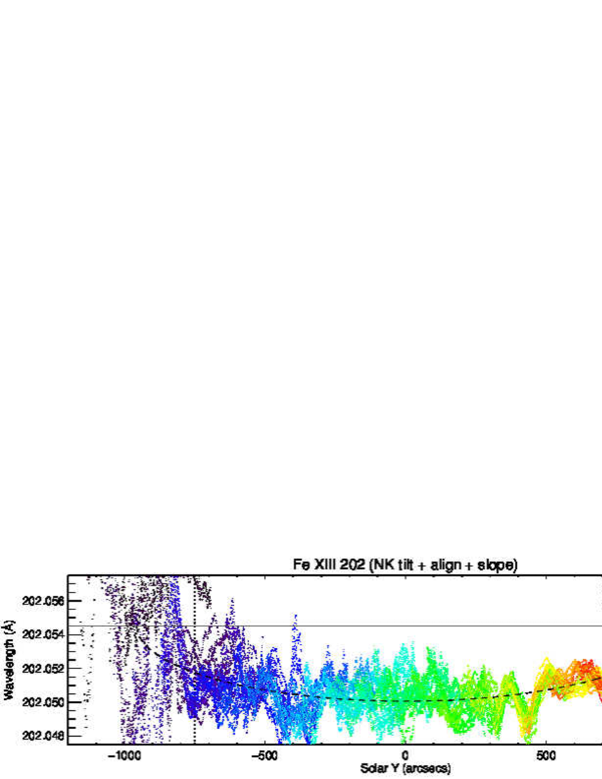
Fig. 3.10: Center-to-limb variations of emission line centroid obtained from the north–south scan during HOP79 in 2010 December. Panels are in the same format as in Fig. 3.9.

We obtained the center-to-limb variations from the north–south scan during HOP79 after analyzing the data as described above. Here results for five emission lines are respectively shown in Fig. 3.9 and Fig. 3.10 with an order of the formation temperature from upper panel to lower one: Fe viii $186.60$Å, Fe x $184.54$Å, Fe xi $188.21$Å, Fe xii $192.39$Å, and Fe xiii $202.04$Å. In those observations, there were no active regions along the meridional line on the solar disk.

Dashed lines in each panel represent the fitted curve when the center-to-limb variation of the Doppler shift is considered to be caused by the radial flow in the solar corona. When the flow is in the radial direction only, the dependence of the Doppler velocity should be $v\,(\theta)=v_{0}\cos\theta$ where $v_{0}$ is the radial velocity and $\theta$ is the angle between line of sight and normal vector as to the solar surface. The solar $Y$ is represented as $y=R_{\odot}\sin\theta$. We fitted the data by converting the abscissa into $\cos\theta$ and applied the linear function. Note that the results were fitted within the range indicated by the region between two vertical dotted lines which indicates the quiet region. There is a small coronal hole at the north pole on 2010 October 7–8 and emission lines are clearly blueshifted at $y\geq 700^{\prime\prime}$ which may be the indication of an outflow. The radial velocity at the disk center is written in the right upper corner of each panel from which we see that the velocity decreases (i.e., upflow becomes stronger) with increasing formation temperature. The indicated errors are those calculated in the fitting procedure from the variance of the data points. We hereafter denote these errors as $\sigma_{\mathrm{fit}}$.

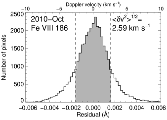
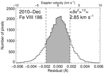
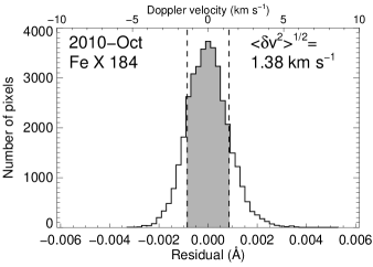
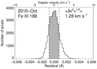
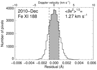
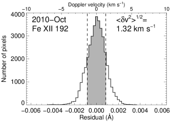
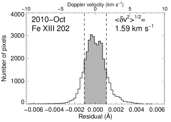
Fig. 3.11: Histograms of residual from the fitted curves in Fig. 3.9 (left column) and Fig. 3.10 (right column). Residuals of Fe viii, and x–xiii are shown in each row. A number $\langle\delta v^{2}\rangle^{1/2}$ in each panel indicates the standard deviation of residual. Two vertical dashed lines indicate $\pm\langle\delta v^{2}\rangle^{1/2}$ and the area between those is painted by gray. Note that data points were extracted from only the fitted region.

Fig. 3.11 shows histograms of the residual from the fitted curves in Fig. 3.9 (October; left column) and Fig. 3.10 (December; right column). Residuals of Fe viii–xiii are shown from upper to bottom panels. A number $\langle\delta v^{2}\rangle^{1/2}$ in each panel indicates the standard deviation of the residual in the unit of $\mathrm{km}\,\mathrm{s}^{-1}$. Two vertical dashed lines indicate $\pm\langle\delta v^{2}\rangle^{1/2}$ and the area between those is painted by gray. The values of $\langle\delta v^{2}\rangle^{1/2}$ are around $1\text{--}3\,\mathrm{km}\,\mathrm{s}^{-1}$, which is much larger than the estimated error of the fitted velocity ($\sigma_{\mathrm{fit}}$) indicated in Fig. 3.9 and Fig. 3.10. Considering that $\langle\delta v^{2}\rangle^{1/2}$ includes the real fluctuation of the quiet region, we regard $\sigma_{\mathrm{tot}}=\left(\sigma_{\mathrm{fit}}^{2}+\langle\delta v^{2}\rangle\right)^{1/2}$ as an error of Doppler velocities at the disk center.

Table 3.1: Doppler velocities at the disk center obtained from north–south scan with Hinode/EIS during 2010. A symbol ^b after wavelength (denoted by Wvl. in the second column) means that the emission line is potentially blended by another emission line. The unit of velocity is $\mathrm{km}\,\mathrm{s}^{-1}$. $\sigma_{\mathrm{fit}}$ is the error in the fitted velocity and $\langle\delta v^{2}\rangle^{1/2}$ is the standard deviation of the residual from the fitted curve. The second column from right shows weighted average which were calculated by using the sum of those two errors squared ($\sigma_{\mathrm{tot}}$ in the text). The most right column shows the error in the weighted average.

			Doppler velocity at the disk center ($\mathrm{km}\,\mathrm{s}^{-1}$)
			October			December
Ion	Wvl. (Å)	$\log T\,[\mathrm{K}]$	$v_{0}$	$\sigma_{\mathrm{fit}}$	$\langle\delta v^{2}\rangle^{1/2}$	$v_{0}$	$\sigma_{\mathrm{fit}}$	$\langle\delta v^{2}\rangle^{1/2}$	Average	Error
Fe viii	$186.60$	$5.69$	$-1.57$	$0.09$	$2.59$	$-0.35$	$0.13$	$2.85$	$-1.02$	$1.92$
Si vii	$275.35$	$5.80$	$-2.45$	$0.10$	$2.86$	$4.56$	$0.16$	$3.41$	$0.44$	$2.19$
Fe ix	$188.49$	$5.92$	$1.00$	$0.06$	$1.73$	$1.55$	$0.09$	$1.92$	$1.25$	$1.29$
Fe x	$184.54$	$6.04$	$-1.59$	$0.05$	$1.38$	$-1.84$	$0.06$	$1.37$	$-1.72$	$0.97$
	$257.26$		$-3.63$	$0.08$	$2.05$	$-2.09$	$0.09$	$1.91$	$-2.81$	$1.40$
Fe xi	$180.40^{\mathrm{b}}$	$6.12$	$-2.24$	$0.07$	$2.07$	$0.48$	$0.09$	$2.00$	$-0.83$	$1.44$
	$188.21$		$-3.18$	$0.04$	$1.28$	$-1.12$	$0.06$	$1.27$	$-2.14$	$0.90$
	$188.30$		$-3.26$	$0.06$	$1.34$	$-0.44$	$0.06$	$1.31$	$-1.82$	$0.94$
Fe xii	$192.39$	$6.19$	$-5.49$	$0.05$	$1.32$	$-3.18$	$0.06$	$1.28$	$-4.30$	$0.92$
	$195.12^{\mathrm{b}}$		$-2.38$	$0.05$	$1.29$	$-0.05$	$0.07$	$1.44$	$-1.34$	$0.96$
Fe xiii	$202.04$	$6.25$	$-6.66$	$0.06$	$1.59$	$-6.57$	$0.09$	$1.91$	$-6.62$	$1.22$

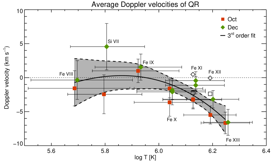
Fig. 3.12: Doppler velocities at the disk center as a function of the formation temperature. Red squares (Green diamonds) indicate October (December) data. Black symbols show the results for potentially-blended emission lines Fe xi $180.40$Å and Fe xii $195.12$Å. The Solid line indicates a third order polynomial function fitted to all data points except for Fe xi $180.40$Å and Fe xii $195.12$Å. The gray region between two dashed lines shows the standard deviation in the fitted curve.

Obtained Doppler velocities from eleven emission lines for the temperature range $\log T\,[\mathrm{K}]=5.7$–$6.3$ are listed in Table 3.1 and these results were plotted in Fig. 3.12. The October and December results are respectively indicated by red squares and green diamonds. December results are shifted by $+0.01$ in abscissa ($\log T\,[\mathrm{K}]$) to facilitate visualization. The vertical error bars indicate $\sigma_{\mathrm{tot}}$. The horizontal error bars indicate the full width of half maximum of contribution function. The Doppler velocities of two potentially blended emission lines Fe xi $180.40$Å and Fe xii $195.12$Å are indicated by black symbols. As being considered in Section 3.3.1.2, those emission lines are redshifted by several $\mathrm{km}\,\mathrm{s}^{-1}$ compared to the isolated emission line from the same ion. The Solid line indicates a third order polynomial function fitted to the all data points except for Fe xi $180.40$Å and Fe xii $195.12$Å. The gray region between two dashed lines shows the standard deviation in the fitted curves. The important conclusion here is that the Doppler velocities are almost zero or slightly positive (i.e., downward) at the temperature below $\log T\,[\mathrm{K}]=6.0$, and above that temperature the emission lines are blueshifted with increasing temperature, and the Doppler velocity reaches ${-7}\,\text{--}\,{-6}\,\mathrm{km}\,\mathrm{s}^{-1}$ at $\log T\,[\mathrm{K}]=6.25$ (Fe xiii).

3.5 Summary

In order to determine the reference velocities for emission lines in the quiet region, we analyzed the data taken during HOP79. The consecutive scans on the meridional line enable us to investigate the center-to-limb variations of spectra. We derived the center-to-limb variations of the Doppler velocities for the emission lines whose formation temperature is above $\log T\,[\mathrm{K}]\geq 6.0$ for the first time. It is concluded that below the temperature of $\log T\,[\mathrm{K}]=6.0$ the Doppler velocities are almost zero or slightly positive (i.e., downward), while the Doppler velocity clearly becomes negative up to $-6\,\mathrm{km}\,\mathrm{s}^{-1}$ above that temperature. Previous observations have shown that the Doppler velocity in the quiet region at $\log T\,[\mathrm{K}]=5.8$ measured by using Ne viii $770.43$Å is $-2.6\pm 2.2\,\mathrm{km}\,\mathrm{s}^{-1}$ (Peter 1999), $-2.4\pm 1.5\,\mathrm{km}\,\mathrm{s}^{-1}$ (Peter & Judge 1999), and $-1.9\pm 2.0\,\mathrm{km}\,\mathrm{s}^{-1}$ (Teriaca et al. 1999). Our results were in good agreement with those studies within the error.

The results obtained in this chapter will be used as a reference for the Doppler velocities of the outflow region at the edge of an active region measured in the next chapter. Although the results themselves would have much importance on the coronal dynamics as discussed in the literature (Peter & Judge 1999), we do not discuss our results further since that is not the main purpose of this thesis.

Appendix 3.A Calibration of the spectrum tilt

EIS slits and CCDs are known to be slightly tilted from the solar $Y$ direction, which creates a systematic shift in observed spectra (hereafter referred to as the spectrum tilt) in CCD $Y$ direction. Since the projection of the slit is tilted clockwise on the CCDs, the spectra is redshifted in the northern part and blueshifted in the southern part. The standard SSW package corrects this effect by referring the tilt derived by the study CALIB_SLOT_SLIT (EIS study No. 352) which was designed to calibrate the the slit tilt and the instrumental width from the off-limb spectra (Young 2010).

There are two remained problems in that calibration: one is that it is unclear whether the spectrum tilt has a dependence on wavelength, and the other is that the spectrum tilt in the long-wavelength (LW) CCD was not investigated. The current standard EIS software uses a single set of fitted parameters derived from Fe xii $193.51$Å/$195.12$Å in the short-wavelength (SW) CCD to calibrate the spectrum tilt. Note that Kamio et al. (2010) investigated the tilts of both CCDs and it was concluded that the SW CCD is more tilted than the LW CCD. In our analysis, we analyze the same data as Kamio et al. (2010) taken at the quiet region near the solar disk and investigate the spectrum tilt using ten emission lines from the two CCDs. The results obtained in this appendix are used to calibrate the spectrum tilt when we deduce the center-to-limb variation of the line centroids (Section 3.3).

3.A.1 Observation and data analysis

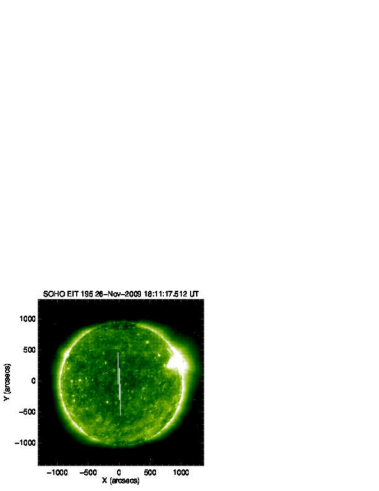
Fig. 3.13: EIT image taken on 2009 November 26 18:11:17UT. Vertical lines indicate the location of EIS pointing during the observation. Three lines are drawn which indicate the pointings. Note that the slight shift of the three lines is imposed for visibility. Those are overlapped completely in the actual observation.

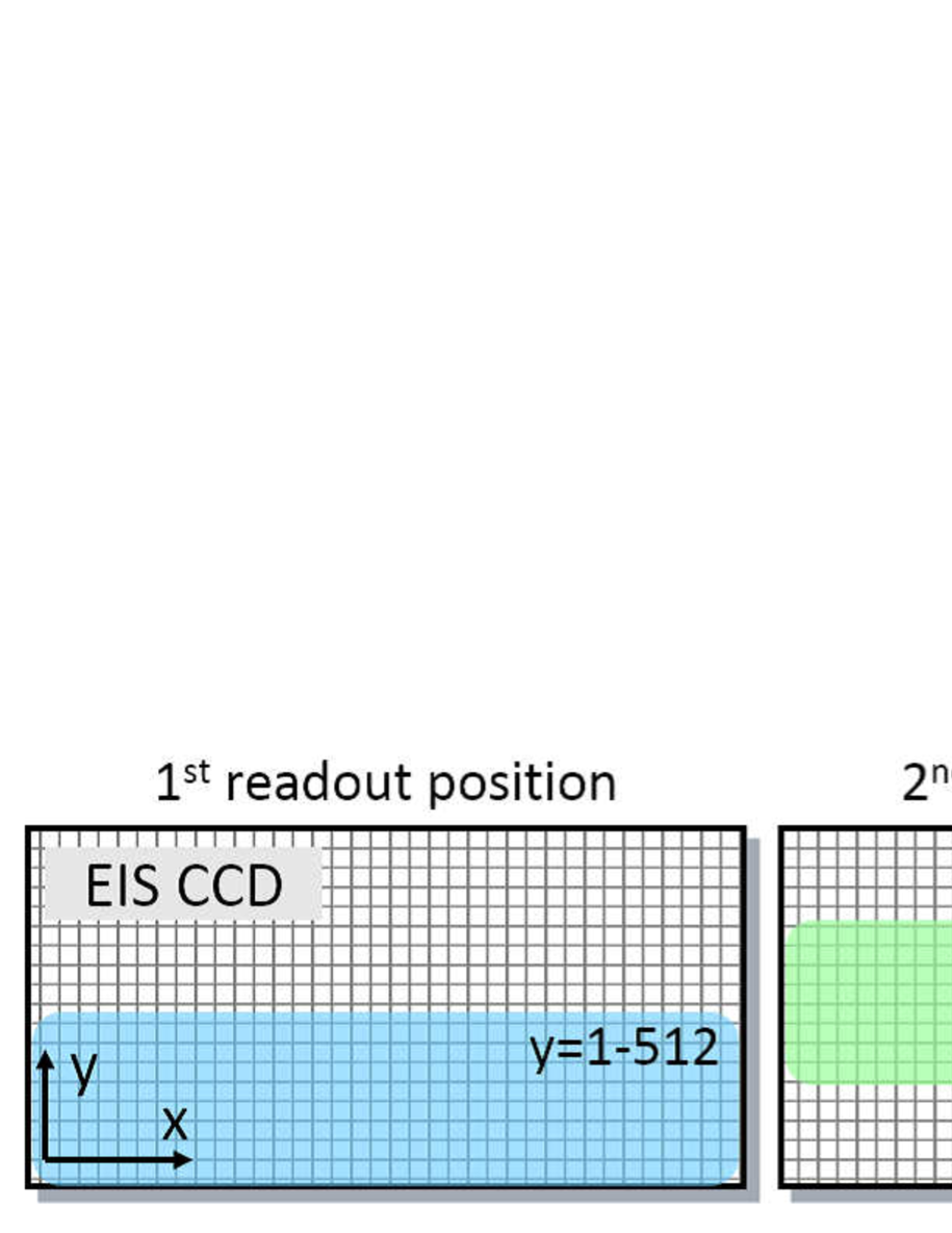
Fig. 3.14: Schematic picture of the EIS observation used to calibrate the spectrum tilt.

In order to calibrate the spectrum tilt, we used the data taken by the same EIS study as that analyzed to investigate the Doppler shifts of the quiet region (north–south scans in HOP79). The data was taken on 2009 November 26. While data taken during HOP79 recorded the spectra with the spatial span of $512$ pixels in $y$ direction ($y=306$–$817$ on the CCDs), this data contains spectra at all $y$ position on the CCDs. This enables us to investigate the spectrum tilt along the EIS slit more precisely. The analysis assumes that the variation of line centroids in the data comes from the instrumental effect, since the variation of the Doppler shift near the disk center is small even if the plasma has a constant radial velocity. The region studied is within approximately $500^{\prime\prime}$ from the disk center, so the curvature produced by the radial velocity does not exceed $1.5\,\mathrm{km}\,\mathrm{s}^{-1}$ when the velocity is $\lesssim 10\,\mathrm{km}\,\mathrm{s}^{-1}$. A context image of the Sun is shown in Fig. 3.13 in which the location of the EIS slit is shown by white line. There were no active regions on the solar disk during the observation.

Since EIS can obtain spectra of $512^{\prime\prime}$ height in the maximum at one exposure, the exposures are divided into three times and take the spectra on pixels $1$–$512$, $256$–$767$, and $511$–$1022$ from the bottom of the CCDs as shown in Fig. 3.14. The spectra were integrated by $50$ pixels in order to enhance S/N ratio when they are fitted by a single Gaussian. At each $y$ position, EIS took the spectra in neighboring five location within $5^{\prime\prime}$ in the east-west direction. The fitted line centroids in these five exposures show almost the same behavior as seen in Fig. 3.15. In order to compensate the influence of the orbital variation, we aligned those five arrays of the line centroid so that the sum of squared difference between each array becomes the minimum. In the next, assuming that the velocity in the quiet region is steady, we connected the three parts of the data and obtained the line centroid as a function of all $y$ position on the CCDs.

3.A.2 Results

3.A.2.1 Spectrum tilt in the short-wavelength CCD

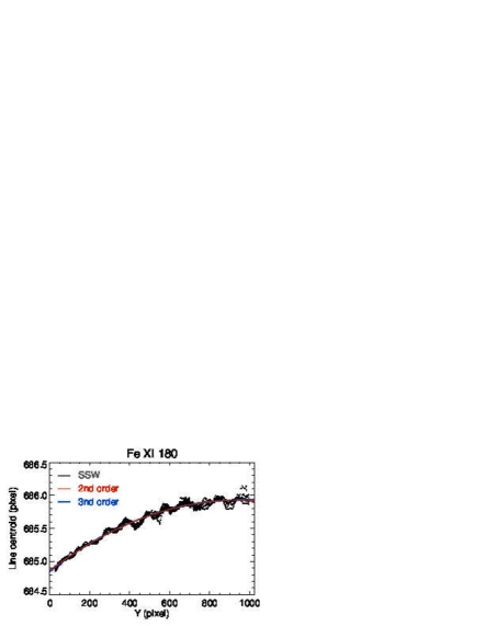
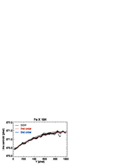
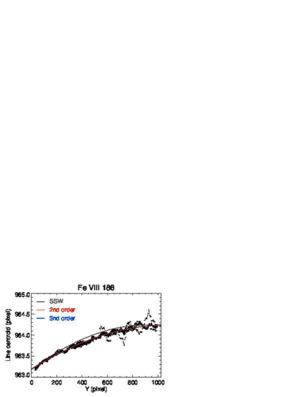
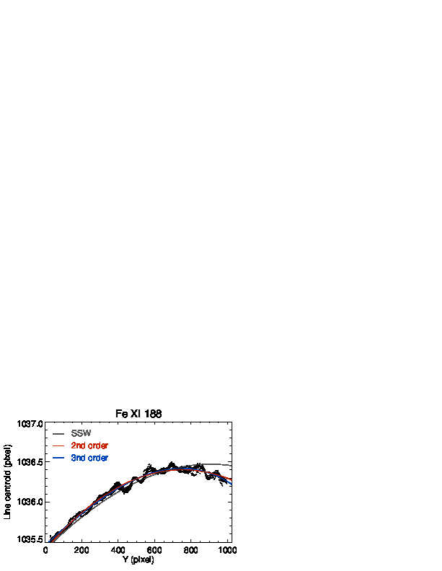
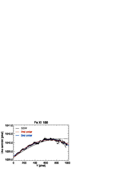
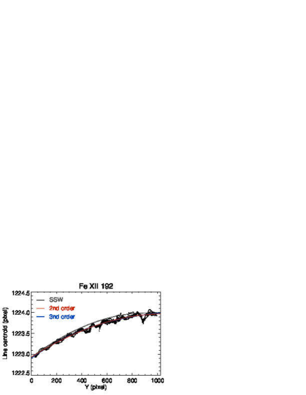
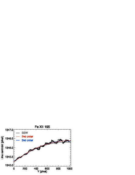
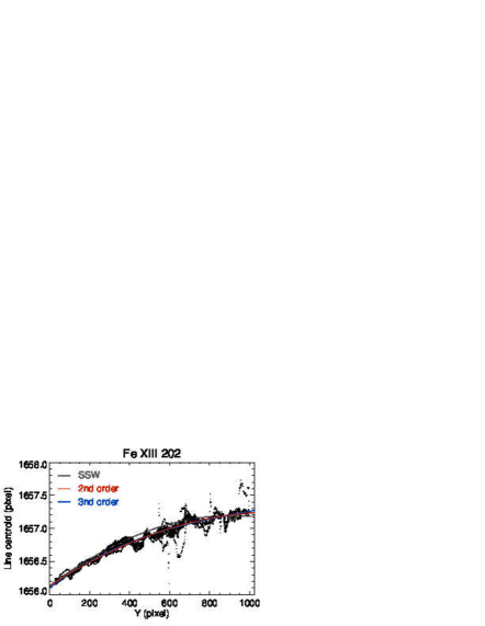
Fig. 3.15: Line centroid as a function of $y$ position on the SW CCD. In each panel, data points are indicated by black dots. Gray, blue, and red lines respectively show the spectrum tilt returned by the standard EIS software, second order polynomial fitting, and third order polynomial fitting.

Line centroids of the emission lines in the SW CCD are shown in Fig. 3.15. Panels show the line centroid as a function of $y$ position on the CCD. Data points are indicated by black dots. Gray, blue, and red lines respectively show the spectrum tilt returned by the standard EIS software, second order polynomial fitting, and third order polynomial fitting. Note that the line centroids are plotted in the unit of spectral pixel which corresponds to $\sim 0.0223$Å $\mathrm{pix}^{-1}$.

All emission lines analyzed here indicate the similar behavior as clearly seen: the line centroids increases from the bottom of the CCD to the top, and they have the curvature with upwardly convex shape. Among them, the line centroid of Fe xi $188.21$Å/$188.30$Å shows different behavior at the top of the CCD above the pixel number around $800$. The curvature is larger than that of other emission lines and only the line centroid of Fe xi $188.21$Å decreases significantly at that location. Another emission line from the same ion Fe xi $180.40$Å did not show such behavior, from which we concluded that this abnormal curvature does not arise from the solar feature but the instrumental effect. We concluded that third order polynomial fitting is better than second order polynomial fitting because the spectrum curvatures seen in Fig. 3.15 may be asymmetric in the $y$ direction.

The third order polynomial functions fitted to each spectrum tilt in the SW CCD are plotted together in Fig. 3.16. Colors indicate the tilt obtained from each emission line. Panel (a) shows the fitted functions and panel (b) shows their derivative. As described above, it is easily seen that the behavior of Fe xi $188.21$Å differs from other emission lines at the top of the CCD. The graph for Fe xii $195.12$Å (indicated by black line) has steeper gradient in the middle of the CCD as seen from panel (b). The standard EIS software calibrates the spectrum tilt by using the result from Fe xii $193.51$Å/$195.12$Å. It means that the spectrum tilt is usually corrected too much for emission lines other than Fe xii $195.12$Å (though the deviation could be reduced by using not only $195.12$Å but also $193.51$Å). From these results, we concluded that it is better to use each fitted spectrum tilt to calibrate each emission line. We used the fitted parameters obtained by third polynomial fitting for each emission line to calibrate the data in HOP79.

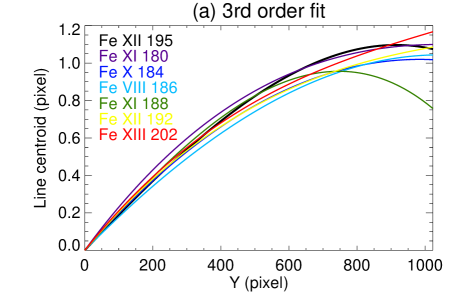
Fig. 3.16: Derivatives of line centroid as a function of $y$ position on the SW CCD.

3.A.2.2 Spectrum tilt in the long-wavelength CCD

The spectrum tilt of the LW CCD is known to have a different property from that of the SW CCD (Kamio et al. 2010), though it is not reflected in the standard EIS software. We investigated two line centroids of Fe x $257.26$Å and Si vii $275.35$Å which are shown in Fig. 3.17. Both panels show the line centroid as a function of $y$ position on the CCD. Data points are indicated by black dots. Gray, blue, and red lines respectively show the spectrum tilt returned by the standard EIS software, second order polynomial fitting, and third order polynomial fitting. Comparing the data to gray lines, it is clear that the spectrum tilt in the LW CCD is much smaller than that in the SW CCD. The results shown here are consistent with those by Kamio et al. (2010). As same as for results in the SW CCD, we used the fitted parameters for each emission line to calibrate the data in HOP79.

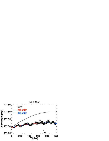
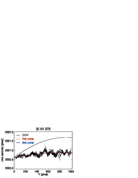
Fig. 3.17: Line centroid as a function of $y$ position on the LW CCD.

3.A.3 Summary

We investigated the spectrum tilts from ten emission lines (eight from the SW CCD and two from the LW CCD) using the data taken at the quiet region near the disk center. The spectra were obtained covering all $y$ position on the CCDs, from which we could analyze the behavior of line centroid along the slit. Our analysis revealed that the spectrum tilt has some characteristic dependence on wavelength. The difference of the tilt in the SW CCD and the LW CCD was also derived which is consistent with the result of Kamio et al. (2010). We use the spectrum tilt obtained here to calibrate the data since the analysis in this chapter dealt the Doppler shifts in the quiet region which is more or less several $\mathrm{km}\,\mathrm{s}^{-1}$ and requires much carefulness for the line centroid compared to other studies. The other reason why we must be such careful is that we investigate the center-to-limb variation of line centroids, which means that even subtle deviation which does not matter in the data with small field of view would become large enough to produce systematic variation in the long distance up to $2000^{\prime\prime}$.

Appendix 3.B Oxygen lines ($\log T\,[\mathrm{K}]=5.4$)

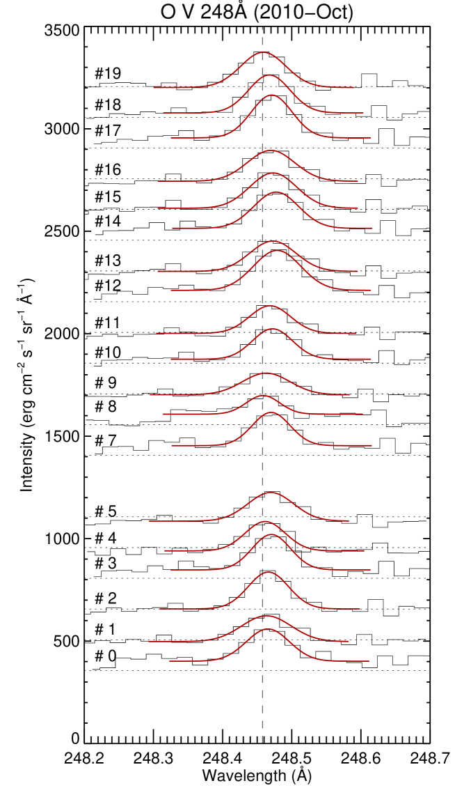
Fig. 3.18: The spectra of O v $248.48$Å integrated by $500^{\prime\prime}$ in the solar $Y$ direction. Twenty spectra were obtained in each pointing from south (#0) to north (#19). Red curves respectively indicate a fitted Gaussian. A vertical dashed line is located at the average wavelength between the spectra #0 and #19.

As introduced in Section 3.3.1.1, there are two transition region lines from oxygen ion in the EIS data analyzed in this chapter. In order to check the consistency of our results and those from previous observations, here we investigated a center-to-limb variation of O v $248.48$Å. This emission line is stronger than O iv $279.93$Å, but in order to obtain the spectra with high S/N ratio which leads to the precision of $\leq 5\,\mathrm{km}\,\mathrm{s}$, we needed spatial integration with $500^{\prime\prime}$ in the solar-Y direction (i.e., along the EIS spectroscopic slit). After the integration, five spectra at each pointing were obtained, which means we obtained $100$ spectra from twenty pointing locations in total. The integrated spectra of O v $248.48$Å at first exposure in each pointing from October data are shown in Fig. 3.18. Twenty spectra were obtained in each pointing from south (#0) to north (#19). Note that the spectrum #6 was absent in this data due to data loss. Red curves plotted over the spectra are a fitted Gaussian. A vertical dashed line is located at the wavelength at the limb as calculated by fitting the result as same as for coronal lines. The spectra at the solar disk are redshifted relative to those near both limbs.

The centroid of the fitted Gaussian as a function of the solar $Y$ coordinate is shown in Fig. 3.19. The line centroids are basically more redshifted at the solar disk than at the limb. Previous observations by SUMER reported the redshift of the transition region lines whose formation temperatures are similar to that of O v (Chae et al. 1998; Peter & Judge 1999). However, we notice that there is a peculiar tendency in the center-to-limb variation of the Doppler shift. The line centroid indeed increases (i.e., redshifted) from the limb to inside the disk as expected from the previous observations, but at some point it decreases in reversal toward the disk center.

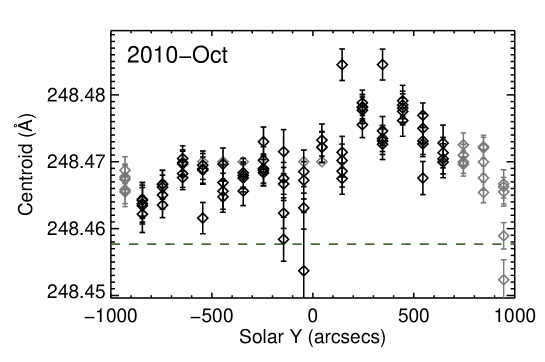
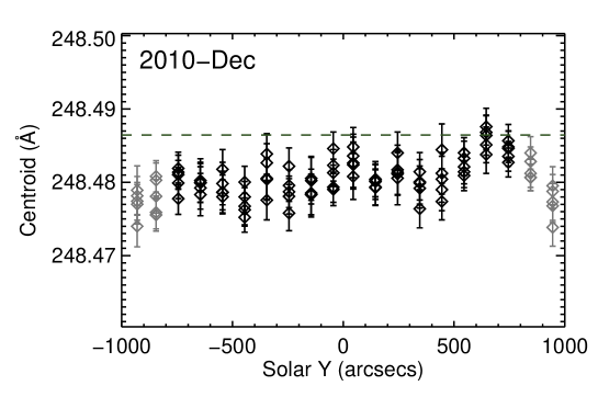
Fig. 3.19: Centroid of O v $248.48$Å as a function of the solar $Y$ coordinate for 2010 October (left) and December (right). Black (Gray) diamonds indicate that those data points are in (out) the quiet region. Green dashed lines are the centroid at the limb derived from the fitting by $v(\theta)=v_{0}\cos\theta$ (cf. Section 3.4).

Chapter 4 Doppler velocity measurement for AR outflows

4.1 Introduction

The solar corona shows different appearance when we observe it in the different temperatures. Focusing on an active region, patchy structures are seen for the temperature of $\log T\,[\mathrm{K}]\leq 5.6$ (i.e., the transition region). For the temperature range of $\log T\,[\mathrm{K}]=5.6$–$6.0$, there are prominent elongated loops structures from the edge of the active region to the surrounding region, named “fan loops” after their appearance. They are often observed at east or west edge of active regions. Going up to higher temperature around $\log T\,[\mathrm{K}]=6.0$–$6.3$, both fan loops and the core of the active region are bright, and loop structures at the core region can be seen which connect positive and negative magnetic polarity. Above the temperature $\log T\,[\mathrm{K}]\simeq 6.4$, radiation from the core region dominates.

The temperature dependence of Doppler velocities gives us a clue to understand the process occurring at the coronal structures. Fan loops are known to indicate characteristic velocity dependence on the temperature (Warren et al. 2011). In the transition region temperature ($\log T\,[\mathrm{K}]\leq 6.0$), they show a redshift of $\sim 10\,\mathrm{km}\,\mathrm{s}^{-1}$ which has been interpreted that the plasma in fan loops around the transition region temperature flows down to the footpoints. On the other hand, a blueshift of $\gtrsim 10\,\mathrm{km}\,\mathrm{s}^{-1}$ is observed above the temperature around $\log T\,[\mathrm{K}]=6.0$ (e.g., Fe x–xv). McIntosh et al. (2012) think this dependence as the indication of the coronal heating followed by cooling. Bradshaw (2008) has analytically estimated the speed of cooling downflow by considering the balance of enthalpy flux, which could account for the reported value of several tens of $\mathrm{km}\,\mathrm{s}^{-1}$.

Since outflow regions often takes its place adjacent to fan loops, and the blueshift of fan loops in corona lines has been reported, outflow regions and fan loops had been often regarded as the identical structure (Tian et al. 2011; McIntosh et al. 2012). Young et al. (2012) recently mentioned that the location of outflows and fan loops are slightly displaced with each other. It was reported that there was no Si vii emission in the outflow region (Warren et al. 2011), which implies that the outflow region could be separated from fan loops. The physical properties of fan loops and the outflows are noted in Table 4.1. We analyzed the data taken at relatively initial phase of Hinode when the sensitivity of EIS was high, and tried to measure the Doppler velocity at the transition region temperature in the outflow region.

Table 4.1: Obtained physical properties and inferences on fan loops and outflows. The results obtained in specific literature are followed by a reference. References are abbreviated as B09 (Baker et al. 2009), NH11 (Nishizuka & Hara 2011), U11 (Ugarte-Urra & Warren 2011), M12 (McIntosh et al. 2012), and Y12 (Young et al. 2012). TR represents the transition region.

	Fan loop	Outflow
Emission lines	Si vii and Fe viii	Fe xi–xv
Temperature ($\log T\,[\mathrm{K}]$)	$5.7\text{--}6.0$	$6.2\text{--}6.3$
Intensity	Bright in TR lines	Dark. Extending structures in Doppler maps of
		coronal lines.
Doppler velocity
The transition region	Downflow of $v\simeq 20\,\mathrm{km}\,\mathrm{s}^{-1}$	Upflow of several $\mathrm{km}\,\mathrm{s}^{-1}$ (B09)
Corona	Upflow or no net velocity (Y12)	Upflow of several tens to a hundred $\mathrm{km}\,\mathrm{s}^{-1}$
Line width	Not studied	Enhanced
Electron density ($\mathrm{cm}^{-3}$)	$5.0\times 10^{8}$ (Y12)	Not studied
Emission line profiles	Symmetric at leg (NH11)	Major component $+$ EBW
	Major component $+$ EBW at footpoint
	(M12)
Inferred origin	Mass draining during the cooling phase	1) Impulsive heating
		2) Reconnection between short and long loops
		3) Horizontal expansion of active regions
		4) Plasma at the tips of chromospheric spicules

In this chapter, we measure the Doppler velocities of a fan loop and the outflow region in NOAA AR10978 using a reference velocity of the quiet region obtained in Chapter 3 and derive the temperature dependence. Previous observations include the error up to $10\,\mathrm{km}\,\mathrm{s}^{-1}$ at most, which might produce even the reversal of the sign of Doppler velocity because the observed values are also the order of $\sim 10\,\mathrm{km}\,\mathrm{s}^{-1}$. Our analysis in Chapter 3 enables us to deduce the Doppler velocity within an error of $\sim 3\,\mathrm{km}\,\mathrm{s}^{-1}$. By measuring the Doppler velocity, we aim to reveal the nature of the outflow region and clarify differences between the outflow region and fan loops. In this thesis, fan loops are defined as the loop structure extending from the periphery of an active region which is bright in the transition region lines, while the outflow region is defined as the region where the emission line width increases in the coronal lines and no fan loops exist.

4.2 Observations and data reduction

4.2.1 EIS scan

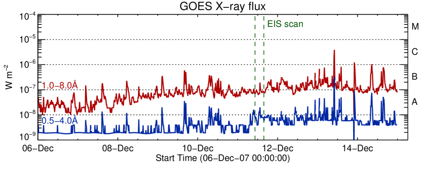
Fig. 4.1: GOES X-ray plot during the disk passage of NOAA AR10978 during 2007 December 6–15. Alphabets written in the right side of the plot denote the conventional classification of flares. Red (Blue) data represents low (high) energy channel of GOES satellite. The interval between green lines indicate the duration of the EIS observation near at the disk center, which was used in this chapter.

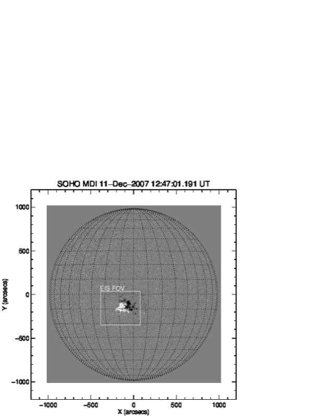
Fig. 4.2: Images of AR10978 taken by SoHO/MDI and EIT. Left: MDI magnetogram taken on 2007 December 11 12:47:01UT. Right: EIT image taken on 2007 December 11 12:00:09UT. The region surrounded by a white dotted line in each panel indicates the field of view (FOV) of an EIS scan analyzed in this chapter.

A raster scan of NOAA AR10978 obtained with Hinode/EIS was analyzed to study the temperature dependence of the Doppler velocity in the outflow region. The active region appeared on the solar disk from the east limb on 2007 December 6, and disappeared into the west limb on 2007 December 18. During this period, no other active regions existed, and the observation by Hinode were focused on AR 10978 except for a few synoptic observations. AR10978 showed overall low activities especially in the former half of its disk passage as shown in Fig. 4.1 (one B-class flare during the scan). There is a negative-polarity leading sunspot and following positive-polarity strong magnetic field regions. A magnetogram and an EUV image of the whole Sun taken by SoHO on 2007 December 11 are shown in Fig. 4.2.

The EIS data analyzed in this chapter was taken on 2007 December 11 10:25:42–15:44:33UT. The scan has a large-area FOV ($460^{\prime\prime}\times 384^{\prime\prime}$) which includes entire AR10978. The $1^{\prime\prime}$ spectroscopic slit was used with an exposure time of $40\,\mathrm{sec}$. The center of the field of view was $(-175^{\prime\prime},-155^{\prime\prime})$, which is suitable to derive the Doppler velocities with less superposition of coronal structures.

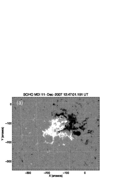
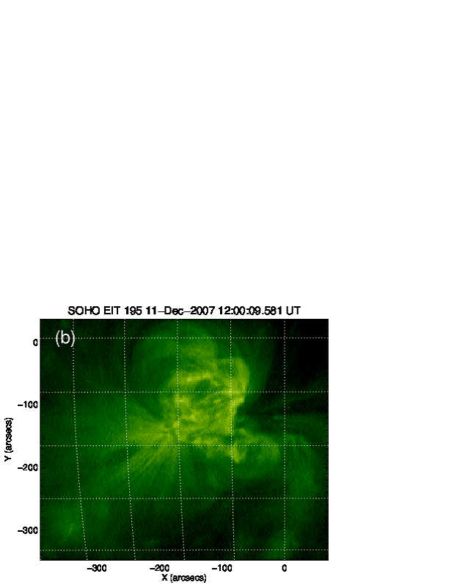
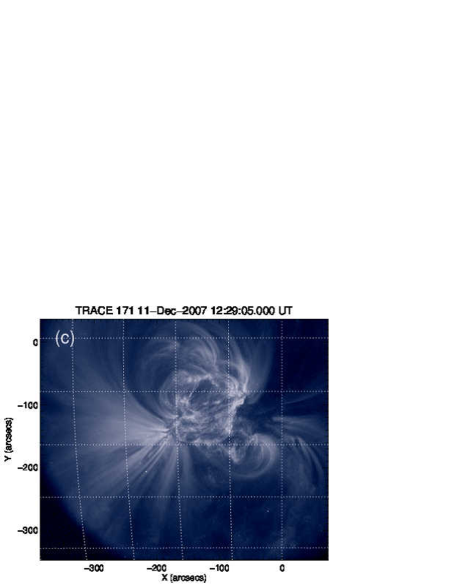
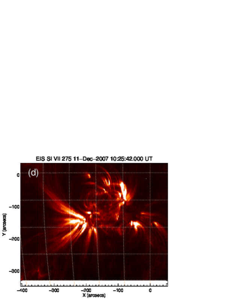
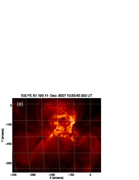
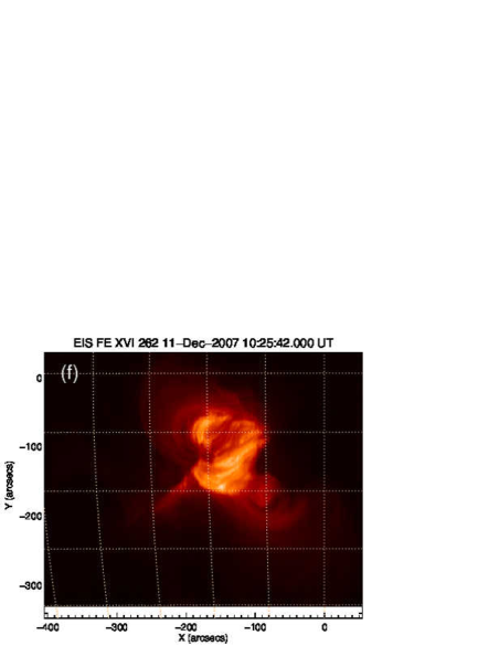
Fig. 4.3: (a) MDI magnetogram, (b) EIT $195$Å passband image, (c) TRACE $171$Å passband image (mainly contributed by Fe ix–x), and intensity maps of three emission lines whose formation temperature is different: (d) Si vii $275.35$Å ($\log T\,[\mathrm{K}]=5.8$), (e) Fe xii $195.12$Å ($\log T\,[\mathrm{K}]=6.2$), and (f) Fe xvi $262.98$Å ($\log T\,[\mathrm{K}]=6.5$).

Fig. 4.3 shows (a) an MDI magnetogram, (b) an EIT $195$Å passband image, (c) a TRACE $171$Å passband image, and (d)–(f) intensity maps of three emission lines whose formation temperature is different: Si vii $275.35$Å ($\log T\,[\mathrm{K}]=5.8$), Fe xii $195.12$Å ($\log T\,[\mathrm{K}]=6.2$), and Fe xvi $262.98$Å ($\log T\,[\mathrm{K}]=6.5$). In the Si vii map, several elongated structures from east and west edge of the active region are seen, which is called as “fan loops”. This structure is typical around this temperature range ($\log T\,[\mathrm{K}]\lesssim 6.0$). The emission from Si vii is relatively dark at the core of the active region. The morphology becomes more complex for the intensity map of Fe xii than that of Si vii. Not only the elongated structure, which is less clearly discernible than fan loops, but also loop-like structure (coronal loops) connecting east and west part of the active region can be seen. Above the temperature around $\log T\,[\mathrm{K}]=6.4$, the emission from the core region dominates over the surroundings as seen in the intensity map of Fe xvi. Emission outside the core region from this temperature range was very weak.

4.2.2 Data reduction

Table 4.2: Emission lines used in this chapter. A symbol (^b) after wavelength indicates that the emission line is blended by another ion at the active region core. The numbers after temperature represent the full width of half maximum of each contribution function $G(T)$.

Ion	Wavelength	Temperature
	(Å)	($\log_{10}\,\mathrm{K}$)
Mg v	$276.58^{\mathrm{b}}$	$5.50_{-0.14}^{+0.14}$
Mg vi	$268.99$	$5.66_{-0.13}^{+0.13}$
Mg vii	$278.40^{\mathrm{b}}$	$5.80_{-0.13}^{+0.13}$
Si vii	$275.35$	$5.80_{-0.13}^{+0.14}$
Si x	$258.37$	$6.15_{-0.11}^{+0.11}$
S x	$264.23$	$6.18_{-0.13}^{+0.13}$
S xiii	$256.69$	$6.42_{-0.10}^{+0.11}$
Fe viii	$185.21^{\mathrm{b}}$, $186.60^{\mathrm{b}}$, $194.66$	$5.69_{-0.17}^{+0.21}$
Fe ix	$188.49$, $197.86$	$5.92_{-0.17}^{+0.15}$
Fe x	$184.54$, $257.26$	$6.04_{-0.13}^{+0.12}$
Fe xi	$182.17$, $198.54$	$6.13_{-0.11}^{+0.11}$
Fe xii	$192.39$, $193.51$, $195.12^{\mathrm{b}}$, $196.64$	$6.19_{-0.10}^{+0.10}$
Fe xiii	$196.54$, $202.04$	$6.25_{-0.09}^{+0.09}$
Fe xiv	$264.789$, $274.20$	$6.30_{-0.09}^{+0.09}$
Fe xv	$284.163$	$6.35_{-0.10}^{+0.11}$
Fe xvi	$262.976$	$6.45_{-0.13}^{+0.20}$
Total	$26$ lines

We used twenty six emission lines in total whose formation temperature ranges widely within $\log T\,[\mathrm{K}]=5.6\text{--}6.5$ in order to investigate temperature dependence of the Doppler velocity in coronal structures without gaps in temperature as long as possible. The emission lines are listed in Table 4.2. We selected emission lines which are relatively strong, isolated and free from significant blend by other unidentified lines. The contribution functions of the emission lines used in this study are shown in Fig. 4.4. Blue, red, yellow, and green lines respectively indicate those of Mg, Si, S, and Fe ion.

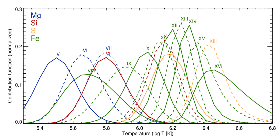
Fig. 4.4: Contribution functions $G(T)$ given by CHIANTI database ver. 7 (Dere et al. 1997; Landi et al. 2012). $G(T)$ for all emission lines used in this chapter are plotted. Colors indicate ion species (blue: Mg, red: Si, yellow: S, and green: Fe). Each contribution function was normalized so that the area under the curve becomes unity.

The data was calibrated through the standard EIS software to remove hot/warm pixels, subtract dark current and CCD pedestal. Note that some programs in the current standard software calibrate the spectrum tilt by using same parameters in both SW and LW CCDs, however, we used different parameters for each CCD given by Kamio et al. (2010). The validity of them was checked as described in Section 4.A.

We focused on four kinds of coronal structure in this chapter: active region core, fan loop, outflow region, and the quiet region. The active region core was defined by the loop system at the center of the active region which is bright in the high temperature emission (cf. panel f in Fig. 4.3), which has the size of $\sim 100^{\prime\prime}$ in the projected plane. In Fe xii and Si vii intensity map (panel d and e in Fig. 4.3), there are no clear loops at the active region core, while patchy structures are seen. Fan loops are extracted from Si vii image in which they are most distinct. We define outflow region as the location (1) where the line width of Fe xii $192.39$Å is enhanced, and (2) which can be spatially separated from fan loops. Several regions were extracted from the raster scan which are indicated by white boxes in Fig. 4.5. Names written beside the boxes respectively means C1–C3: active region core, F1–F4: fan loop, and U1–U4: outflow region. As the quiet region, we selected the region far from the active region as long as possible, which is indicated by the box named QR. The size of the boxes was chosen so that they fit to the spatial size of target structures (C1–C3, F1–F4, and QR: $20^{\prime\prime}\times 20^{\prime\prime}$, U1 and U2: $12^{\prime\prime}\times 12^{\prime\prime}$, U3–U4: $15^{\prime\prime}\times 15^{\prime\prime}$). Since fan loops were well developed at the east edge, so we carefully select the location of the outflow regions U1 and U2 in order to avoid the influence of neighboring fan loops.

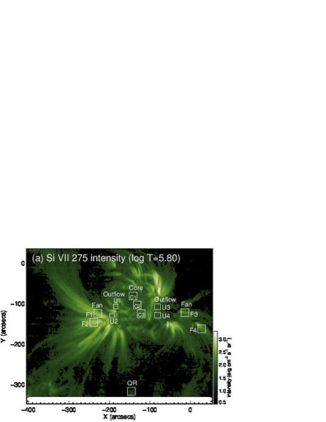
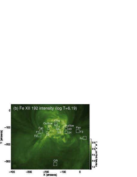
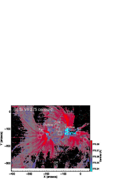
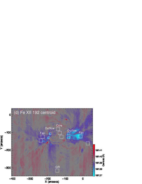
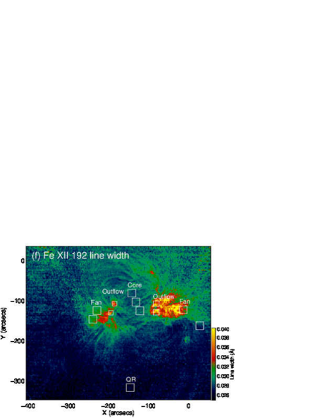
Fig. 4.5: Maps of intensity (upper), line centroid (middle), and line width (lower). Left panels show those for (a) Si vii $275.35$Å and right panels show those for (b) Fe xii $192.39$Å. Boxes in the maps indicate the regions where Doppler velocities were measured in detail: C1–C3: active region core, F1–F4: fan loops, U1–U4: outflow regions, and QR: the quiet region.

4.3 Line profiles

Before measuring Doppler velocities, we look at each emission line profile. Even visual inspection of line profiles gives us an insight sometimes better than a fitting result. We compare line profiles from four locations: the quiet region (QR), fan loops (F1), an active region core (C2), and the outflow region (U3) indicated by white boxes in Fig. 4.5. Maps in the figure show intensity, line centroid, and line width from upper to lower panels. Left and right columns respectively show those for Si vii $275.35$Å ($\log T\,[\mathrm{K}]=5.80$) and Fe xii $192.39$Å ($\log T\,[\mathrm{K}]=6.19$). In the following sections, we show the emission line profiles in an order of the formation temperature and note their characteristics. The spectra from four regions (C2, F1, U3, and QR) were averaged within each region.

4.3.1 $\log T\,[\mathrm{K}]=5.7$–$5.8$

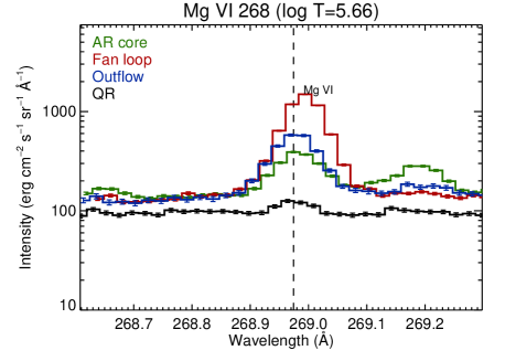
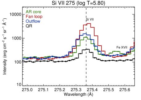
Fig. 4.6: Line profiles at the quiet region (black), the outflow region (blue), a fan loop (red), and the core region (green). Left: Mg vi $268.99$Å. Right: Si vii $275.35$Å. A vertical dashed line in each panel indicates a line centroid of the emission line at the quiet region.

Line profiles of two transition region emission lines Mg vi $268.99$Å ($\log T\,[\mathrm{K}]=5.66$) and Si vii $275.35$Å ($\log T\,[\mathrm{K}]=5.80$) are shown in Fig. 4.6. Black, blue, red, and green histograms respectively indicate the line profile in the quiet region, the outflow region, a fan loop, and the core region which were indicated by white boxes in Fig. 4.5. A vertical dashed line in each panel indicates a line centroid of the emission line at the quiet region. The line profiles for fan loops are clearly shifted toward longer wavelength (i.e., redshift) by around $1\,\mathrm{pix}$ (corresponding to $\simeq 0.022$Å) which corresponds to $\sim 20\,\mathrm{km}\,\mathrm{s}^{-1}$ downward to the solar surface at this wavelength. On the other hand, the line profiles in the outflow region are blueshifted by $\simeq 0.5\,\mathrm{pix}$. The line profiles look like almost symmetric in all regions. It should be noted that those in the outflow region are wider than those in other regions.

4.3.2 $\log T\,[\mathrm{K}]=6.1$–$6.2$

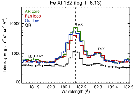
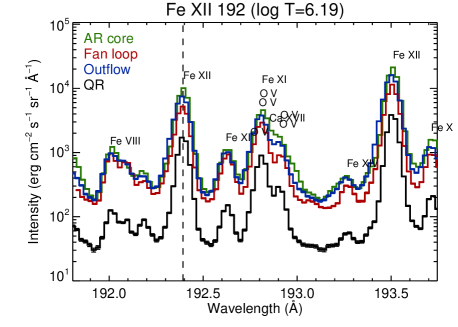
Fig. 4.7: Line profiles at the quiet region (black), the outflow region (blue), fan loop (red), and the core region (green). Left: Fe xi $182.17$Å. Right: Fe xii $192.39$Å. A vertical dashed line in each panel indicates a line centroid of the emission line at the quiet region.

Line profiles of two coronal emission lines Fe xi $182.17$Å ($\log T\,[\mathrm{K}]=6.13$) and Fe xii $192.39$Å ($\log T\,[\mathrm{K}]=6.19$) are shown in Fig. 4.7. Different from the transition region emission lines, they exhibit an enhanced component at their blue wing in the outflow region. This enhancement can be seen up to $4$–$5$ pixels far from the line centroid, which indicates that the upflow with a speed up to $100\,\mathrm{km}\,\mathrm{s}^{-1}$ exists, while major portion of the emission is located near the same centroid as the quiet region where the plasma moves only by $\lesssim 10\,\mathrm{km}\,\mathrm{s}$. Note that the line profiles look symmetric in the quiet region.

The enhanced blue wing is more clearly seen in Fe xii than in Fe xi, which means that the upflow dominantly consists of plasma with a temperature higher than the formation temperature of Fe xi. Another noticeable feature is that the enhanced component in Fe xii has even the same magnitude as the intensity in the core region at around $\lambda=192.30$Å. We can see the similar behavior also for Fe xii $193.51$Å included in this spectral window.

4.3.3 $\log T\,[\mathrm{K}]=6.3$

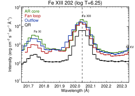
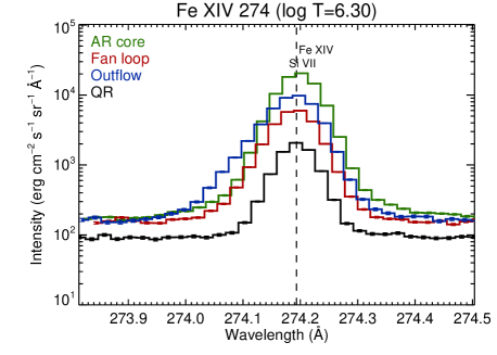
Fig. 4.8: Line profiles at the quiet region (black), the outflow region (blue), fan loop (red), and the core region (green). Left: Fe xiii $202.04$Å. Right: Fe xiv $274.20$Å. A vertical dashed line in each panel indicates a line centroid of the emission line at the quiet region.

Fig. 4.8 shows line profiles for Fe xiii $202.04$Å ($\log T\,[\mathrm{K}]=6.25$) and Fe xiv $274.20$Å ($\log T\,[\mathrm{K}]=6.30$). While the line profiles in the quiet region (black), a fan loop (red), and the core region (green) all look symmetric and their centroid position do not deviate significantly from the value of the quiet region indicated by a vertical dashed line, those in the outflow region (blue) exhibit a significant enhancement in their blue wing (at $\lambda=201.85$–$201.95$Å for Fe xiii and at $\lambda=273.95$–$274.05$Å for Fe xiv) similar to Fe xi–xii. Note that major portion of the emission is again located near the line centroid in the quiet region (i.e., at the vertical dashed line).

4.3.4 $\log T\,[\mathrm{K}]=6.4$–$6.5$

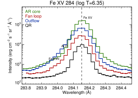
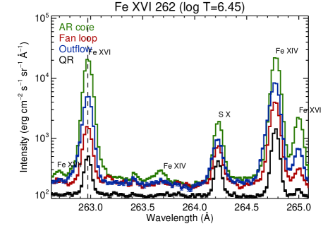
Fig. 4.9: Line profiles at the quiet region (black), the outflow region (blue), fan loop (red), and the core region (green). Left: Fe xv $284.16$Å. Right: Fe xvi $262.98$Å. A vertical dashed line in each panel indicates a line centroid of the emission line at the quiet region.

The hottest coronal plasma seen in the non-flare condition reaches around the temperature of $\log T\,[\mathrm{K}]\simeq 6.5$, which can be observed by Fe xv $284.16$Å ($\log T\,[\mathrm{K}]=6.35$) and Fe xvi $262.98$Å ($\log T\,[\mathrm{K}]=6.45$). Their line profiles are shown in Fig. 4.9. The line profiles in the quiet region, a fan loop, and the core region respectively indicated by black, red, and green spectrum seem to be symmetric as same as those from lower temperature. Though an enhancement at the blue wing indeed exists around $\lambda=283.85$–$284.00$Å in the Fe xv emission line in the outflow region (blue), that does not exceed the intensity of the core region (green), which differs from the case of Fe xii–xiv ($\log T\,[\mathrm{K}]=6.2$–$6.3$).

Another important feature to be mentioned here is that the enhancement at the blue wing does not exist in the line profile of Fe xvi in the outflow region (blue). These indicates that the plasma producing the enhancement at blue wings in the line profiles have a temperature lower than $\log T\,[\mathrm{K}]\simeq 6.4$. Though not shown in the figure, S xiii $256.69$Å ($\log T\,[\mathrm{K}]=6.42$) also indicates the same characteristic as Fe xvi (i.e., no enhancement at its blue wing).

4.4 Measurement of the Doppler velocities of AR outflows

4.4.1 Doppler velocity maps

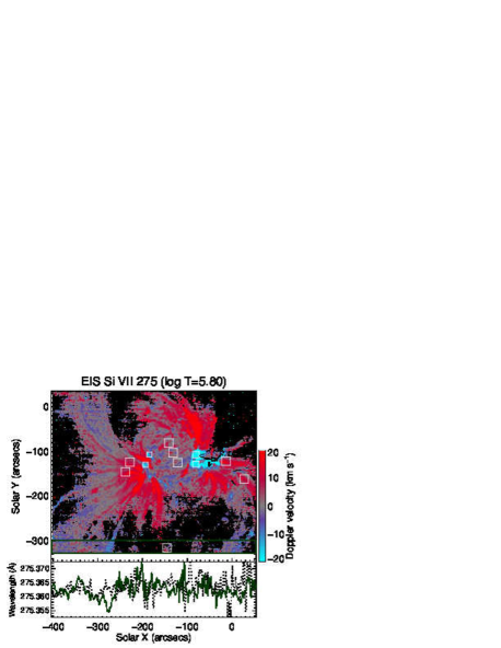
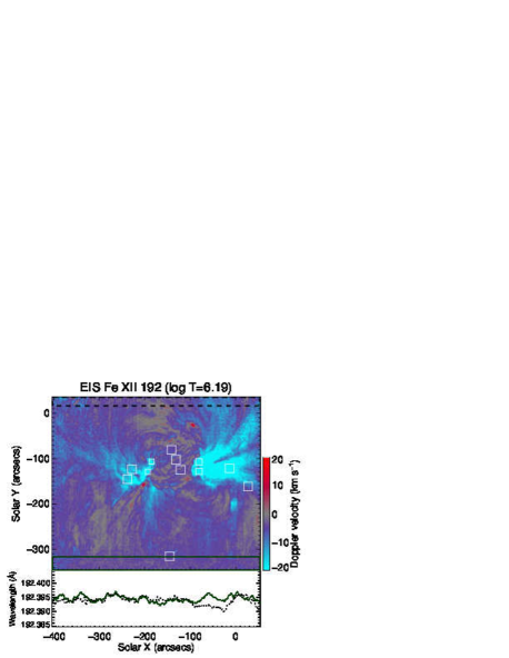
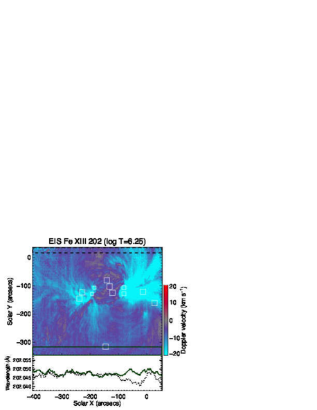
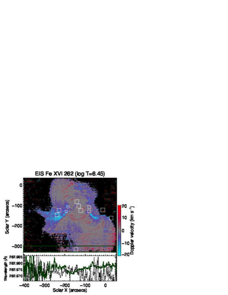
Fig. 4.10: Doppler velocity maps of AR10978. Left upper: Si vii $275.35$Å. Right upper: Fe xii $192.39$Å. Left lower: Fe xiii $202.04$Å. Right lower: Fe xvi $262.98$Å.

We calculated the Doppler velocity $v_{\mathrm{Dop}}$ by using the equation

$$v_{\mathrm{Dop}}=\dfrac{\lambda_{\mathrm{c}}-\lambda_{0}}{\lambda_{0}}c\,\text{,}$$ (4.1)

where $\lambda_{\mathrm{c}}$ is the line centroid, $\lambda_{0}$ is a rest wavelength, and $c$ is the speed of the light. Here the fitting result by a single Gaussian was used for $\lambda_{\mathrm{c}}$. This means that the Doppler velocity derived for the outflow region could be a weighted average of multiple components in the line profile, which leads to the speed of the outflow itself underestimated in the absolute value because there is a major component with much little shift. The deviation from the single Gaussian fitting for a coronal emission line is described in Appendix 4.D.

The Doppler velocity map for Si vii $275.35$Å ($\log T\,[\mathrm{K}]=5.80$), Fe xii $192.39$Å ($\log T\,[\mathrm{K}]=6.19$), Fe xiii $202.04$Å ($\log T\,[\mathrm{K}]=6.25$), and Fe xvi $262.98$Å ($\log T\,[\mathrm{K}]=6.45$) are shown in Fig. 4.10. The line profiles were spatially integrated by $3\times 3\,\mathrm{pix}^{2}$ before the single Gaussian fitting for Fe emission lines. The regions where the statistical error originated in the photon noise exceeds $5\,\mathrm{km}\,\mathrm{s}^{-1}$ are painted by black. Note that we do not refer to Fe xii $195.12$Å, which is commonly used in the literature, due to the fact that the emission line is contributed by the neighboring Fe xii $195.18$Å at the region where the electron density becomes high (e.g., active region core), and it produces a fake redshift.

The plot below each map in Fig. 4.10 shows the line centroids averaged in $y$ direction within squares indicated by green thick line and black dashed line in Doppler velocity maps. At some locations, the line centroids are shifted coherently by several $\mathrm{m}$Å in these two regions which may be a residual of the orbital variation. In order to compensate those shifts, we subtracted the 5-exposures running average (i.e., in the solar $x$ direction) of the centroid of Fe xii $192.39$Å indicated by the green thick line in the lower plot. This emission line was strong enough to obtain precise centroid ($\sigma\leq 1\,\mathrm{km}\,\mathrm{s}^{-1}$) in the quiet region with spatial average of $3\times 3\,\mathrm{pix}^{2}$. As far as the orbital variation dominantly comes from the spatial displacement of the grating component in the EIS instrument, all emission lines should be shifted by the same amounts. It might be too much subtraction because this process could also remove the real fluctuation in the quiet region, so we set the window size of $5$ exposures in order not to compensate the statistical fluctuation of that size at least.

The references of the Doppler velocity were set to $v_{\mathrm{QR}}=0.2\,\mathrm{km}\,\mathrm{s}^{-1}$ for Si vii, $v_{\mathrm{QR}}=-4.3\,\mathrm{km}\,\mathrm{s}^{-1}$ for Fe xii, $v_{\mathrm{QR}}=-6.3\,\mathrm{km}\,\mathrm{s}^{-1}$ for Fe xiii which were obtained by the procedures in Chapter 3. By adjusting the average Doppler velocity within the region indicated by a green dashed box in the map to be $v_{\mathrm{QR}}$, we have obtained the Doppler velocity map. The map for Fe xii is obviously different from those derived by setting the average Doppler velocity within in the map (or the quiet region) to be zero as in some previous studies, which of course become a mixture pattern of red and blue. Note that since we could not measure the average Doppler velocity of the quiet region for $\log T\,[\mathrm{K}]\geq 6.3$ in Chapter 3, the average Doppler velocity in the green dashed box was set to zero for Fe xvi, which means that the Doppler velocity for Fe xvi is a relative quantity to that of the quiet region.

Doppler velocity maps in Fig. 4.10 show some characteristic patterns. Fan loops extended from both edges of the active region core are clearly redshifted by around $20\,\mathrm{km}\,\mathrm{s}^{-1}$ as seen in the Si vii map. We can see several filamentary structures at around $(-250^{\prime\prime},-180^{\prime\prime})$ and $(30^{\prime\prime},-150^{\prime\prime})$. On the other hand, the outflow regions at $(-80^{\prime\prime},-120^{\prime\prime})$ and around $(-200^{\prime\prime},-150^{\prime\prime})$ are blueshifted by $v=-20\,\mathrm{km}\,\mathrm{s}^{-1}$. Doppler velocity maps for coronal emission lines (i.e., Fe xii, xiii, and xvi) show quite different appearance from that for Si vii. The locations corresponding to fan loops are blueshifted by larger than $20\,\mathrm{km}\,\mathrm{s}^{-1}$. This is common properties within coronal emission lines. In contrast to the map for Si vii, the boundary between fan loops and the outflow region can not distinguished from the Doppler velocity.

4.4.2 Histogram of Doppler velocities

The histograms of the Doppler velocities will be shown here in order to study their characteristics more quantitatively. We show the histograms for the same emission lines as described in Section 4.3 which covers wide temperature range of $\log T\,[\mathrm{K}]=5.7$–$6.5$.

4.4.2.1 $\log T\,[\mathrm{K}]=5.7$–$5.8$

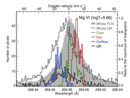
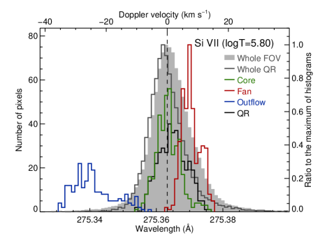
Fig. 4.11: Histogram of line centroid/Doppler velocity at the quiet region (black), the outflow region (blue), fan loop (red), and the core region (green). A gray solid histogram is for the entire quiet region (defined as lower $30$ rows $[\mathrm{pixels}]$ in the map). The histogram filled with gray indicates that for the whole map. Left: Mg vi $268.99$Å. Right: Si vii $275.35$Å. A vertical dashed line in each panel indicates zero point of Doppler velocity which was calculated so as the quiet region has the average Doppler velocity determined in Chapter 3.

Histograms for Mg vi $268.99$Å ($\log T\,[\mathrm{K}]=5.66$) and Si vii $275.35$Å ($\log T\,[\mathrm{K}]=5.80$) are shown in Fig. 4.11. Black, blue, red, and green histograms respectively indicate the result from the quiet region, the outflow region, the fan loop, and the core region within white boxes C2, F1, U3, and QR in Fig. 4.5. A Gray solid histogram is for the entire quiet region defined as lower $30$ rows $[\mathrm{pixel}]$ in the map. The histogram filled with gray indicates that for the whole map. These two histograms were normalized by the maximum value of other four histograms. A vertical dashed line in each panel indicates zero point of Doppler velocity which was determined so that the average Doppler velocity of the quiet region has the average Doppler velocity obtained in Chapter 3.

The histogram for Mg vi in the left panel of Fig. 4.11 shows that the Doppler velocity in the outflow region reaches $-20\,\text{--}\,{-10}\,\mathrm{km}\,\mathrm{s}^{-1}$, while that in the fan loop indicates $10\text{--}20\,\mathrm{km}\,\mathrm{s}^{-1}$ in reversal. The core region shows almost no velocity. The right panel shows the histogram for Si vii. It basically has the same behavior for the selected region as that for Mg vi, but more clearly. The outflow region exhibits the upward speed of $\gtrsim 20\,\mathrm{km}\,\mathrm{s}^{-1}$ and the histogram for this region significantly deviates from that of other regions. On the other hand, the fan loop shows the downward speed around $10\,\mathrm{km}\,\mathrm{s}^{-1}$. The histogram for the core region is located at almost the same position as that for the quiet region.

4.4.2.2 $\log T\,[\mathrm{K}]=6.1$–$6.2$

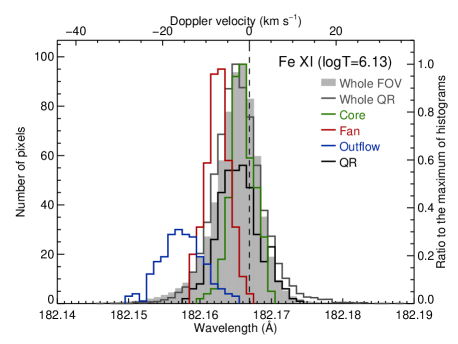
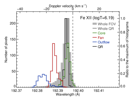
Fig. 4.12: Histogram of line centroid/Doppler velocity at the quiet region (black), the outflow region (blue), fan loop (red), and the core region (green). A Gray solid histogram is for the quiet region (defined as lower $30$ pixels in the map). The histogram filled with gray indicates that for the whole map. Left: Fe xi $182.17$Å. Right: Fe xii $192.39$Å. A vertical dashed line in each panel indicates zero point of Doppler velocity which was calculated so as the quiet region has the average Doppler velocity determined in Chapter 3.

Fig. 4.12 shows histograms for Fe xi $182.17$Å and Fe xii $192.39$Å whose formation temperature is around $\log T\,[\mathrm{K}]=6.1$–$6.2$. While the Doppler velocity for Fe xi is $-10\,\text{--}\,{-5}\,\mathrm{km}\,\mathrm{s}^{-1}$ in the fan loops, that for Fe xii exceeds $-10\,\mathrm{km}\,\mathrm{s}^{-1}$. Though not shown in the figure, a neighbor emission line Fe xii $193.51$Å also shows the same behavior.

Both emission lines exhibit the Doppler velocity of $\simeq-20\,\mathrm{km}\,\mathrm{s}^{-1}$ (i.e., upward) in the outflow region, and the speed is larger for Fe xii than for Fe xi (i.e., higher formation temperature) by roughly $5\,\mathrm{km}\,\mathrm{s}^{-1}$.

4.4.2.3 $\log T\,[\mathrm{K}]=6.3$

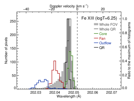
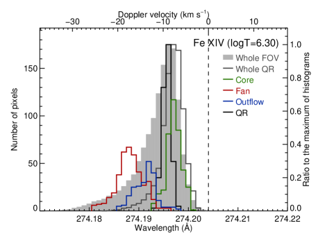
Fig. 4.13: Histogram of line centroid/Doppler velocity at the quiet region (black), the outflow region (blue), fan loop (red), and the core region (green). A Gray solid histogram is for the quiet region (defined as lower $30$ pixels in the map). The histogram filled with gray indicates that for the whole map. Left: Fe xiii $202.04$Å. Right: Fe xiv $274.20$Å. A vertical dashed line in each panel indicates zero point of Doppler velocity which was calculated so as the quiet region has the average Doppler velocity determined in Chapter 3.

The emission lines with the formation temperature around $\log T\,[\mathrm{K}]=6.3$ have the largest enhancement in their blue wing compared to the major component in the line profiles as described in Section 4.3. As shown in Fig. 4.13, the Doppler velocity in the outflow region reaches $\simeq-30\,\mathrm{km}\,\mathrm{s}^{-1}$ for Fe xiii. For Fe xiv, the Doppler velocity there becomes smaller, which is around $-20\,\text{--}\,{-10}\,\mathrm{km}\,\mathrm{s}^{-1}$. The Doppler velocity in the fan loop becomes larger than lower formation temperatures, and indicates blueshift of $v\simeq-20\,\mathrm{km}\,\mathrm{s}^{-1}$ for both emission lines.

Note that the histograms for whole FOV (filled with gray) of the scan have an extended tail toward shorter wavelength for both emission lines, which was previously reported for Fe xiv $274.20$Å (Hara et al. 2008). This property clearly differs from the histograms for the whole quiet region (gray solid) which look symmetric especially for Fe xiii.

4.4.2.4 $\log T\,[\mathrm{K}]=6.4$–$6.5$

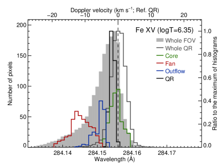
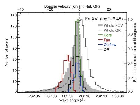
Fig. 4.14: Histogram of line centroid/Doppler velocity at the quiet region (black), the outflow region (blue), fan loop (red), and the core region (green). A Gray solid histogram is for the quiet region (defined as lower $30$ pixels in the map). The histogram filled with gray indicates that for the whole map. Left: Fe xv $284.16$Å. Right: Fe xvi $262.98$Å. The average value in the quiet region was used for zero point of Doppler velocity because we could not determine the reference at this temperature in Chapter 3.

Fig. 4.14 shows the histograms of the Doppler velocity for Fe xv $284.16$Å and Fe xvi $262.98$Å ($\log T\,[\mathrm{K}]\geq 6.4$). While the quiet region, the fan loop, and the core region all have similar value within $\simeq 2$–$3\,\mathrm{km}\,\mathrm{s}^{-1}$, the outflow region exhibits the Doppler velocity around $-15\,\mathrm{km}\,\mathrm{s}^{-1}$ for Fe xv, which is smaller than that of Fe xiii in the magnitude. The Doppler velocity in the fan loop is around $-10\,\mathrm{km}\,\mathrm{s}^{-1}$, and slightly decreases from the temperature of $\log T\,[\mathrm{K}]=6.3$. Note that the histogram obtained from the whole map for Fe xv again has an extended tail as same as for Fe xiv.

One striking fact here is that the outflow ceases for Fe xvi. The histogram for S xiii $256.69$Å (though not shown), which has a similar formation temperature ($\log T\,[\mathrm{K}]=6.42$), exhibited the same behavior as Fe xvi. This reinforces the result that the outflow was significantly reduced at the temperature higher than $\log T\,[\mathrm{K}]=6.4$.

4.5 Temperature dependence of the Doppler velocities

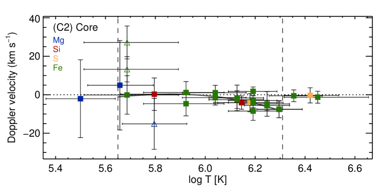
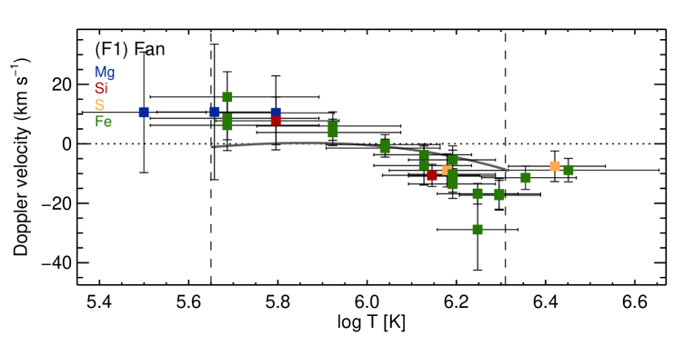
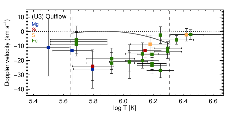
Fig. 4.15: Temperature dependence of the average Doppler velocities. Upper: active region core. Middle: fan loop. Lower: outflow region. Vertical error bars indicate the standard deviation of Doppler velocities in each region including the error in the reference Doppler velocity. Horizontal error bars indicate the full width of half maximum of the contribution functions. Two vertical dashed lines show the range where the reference Doppler velocity was measured in Chapter 3. Triangles in upper panel indicate emission lines blended by a high temperature coronal emission line.

Fig. 4.15 shows the temperature dependence of the Doppler velocities in (a) the core region (C2), (b) fan loop (F1), and (c) the outflow region (U3). The Doppler velocities here are the values averaged within the white boxes indicated in Fig. 4.5. Colors of data points indicate the ion species as denoted in legends. Vertical error bars indicate the standard deviation of Doppler velocities in each region. Those are not calculated from errors originated in Poisson noise of photons which is typically in the order of $1.5\,\mathrm{km}\,\mathrm{s}^{-1}$ (the core region), $2.2\,\mathrm{km}\,\mathrm{s}^{-1}$ (fan loop), and $4.7\,\mathrm{km}\,\mathrm{s}^{-1}$ (the outflow region) for Fe xi $182.17$Å (i.e., medium strength in the studied emission lines). These values are slightly less than the standard deviation shown in each panel, but they are in almost the same magnitude, from which it can be considered that the standard deviation of measured Doppler velocities includes Poisson noise and the physical fluctuation of Doppler velocity in the studied region. Two vertical dashed lines show the range where the reference Doppler velocity was measured in Chapter 3. Since the Doppler velocity above the temperature of $\log T\,[\mathrm{K}]=6.25$ could not determined, we plotted the difference from the quiet region value for Fe xv, S xiii and Fe xvi (i.e., rightmost three data points). The formation temperature of Fe xiv ($\log T\,[\mathrm{K}]=6.30$) is located within the full width of half maximum of the contribution function of Fe xiii, and the Doppler velocity of the quiet region obtained in Chapter 3 was extrapolated for Fe xiv. For Mg v $276.58$Å ($\log T\,[\mathrm{K}]=5.50$) at the low temperature side, we adopted the result from SUMER observation: $v_{\mathrm{QR}}=6.7\,\mathrm{km}\,\mathrm{s}^{-1}$ at $\log T\,[\mathrm{K}]=5.50$ (Teriaca et al. 1999).

In the active region core shown in panel (a), almost all of the emission lines exhibited the Doppler velocities within $-5\,\mathrm{km}\,\mathrm{s}^{-1}\leq v_{\mathrm{Dop}}\leq 5\,\mathrm{km}\,\mathrm{s}^{-1}$. Only exceptions are Mg vii ($\log T\,[\mathrm{K}]=5.80$) which has the velocity of around $-15\,\mathrm{km}\,\mathrm{s}^{-1}$, and Fe viii $185.21$Å and $186.60$Å ($\log T\,[\mathrm{K}]=5.69$) which have the Doppler velocity larger than $10\,\mathrm{km}\,\mathrm{s}^{-1}$. Judging from the spectra of Mg vii at the core region (shown in Appendix 4.B), there seems to exist a P xii emission line ($\log T\,[\mathrm{K}]=6.3$) exists at the blue wing of Mg vii. Note that the spectra other than in the core region do not significantly suffer from those blends as seen in Fig. 4.18. Fe viii $185.21$Å and $186.60$Å are respectively blended by Ni xvi $185.23$Å and Ca xiv $186.61$Å, which are both located near Fe viii lines. Since the separation between Fe viii and blending line is smaller than EIS spectral pixels ($\simeq 0.0223\,\text{\AA}\,\mathrm{pix}^{-1}$), the spectra were not obviously distorted.

The fan loop shows a characteristic dependence as shown in panel (b). We can see clearly downward velocity in lower temperature and upward velocity in higher temperature within the temperature range $\log T\,[\mathrm{K}]=5.7$–$6.3$. This result is consistent with that obtained by Warren et al. (2011). The Doppler velocities above the formation temperature $\log T\,[\mathrm{K}]=6.4$ includes systematic uncertainties due to the fact that we could not determine the zero point of Doppler velocities for emission lines with the formation temperature above $\log T\,[\mathrm{K}]=6.4$ in Chapter 3 because those emission lines were too weak in the quiet region. The Doppler velocities above $\log T\,[\mathrm{K}]=6.4$ represent the relative velocities from those of the quiet region.

Panel (c) shows the temperature dependence of the outflow region, which is our main topic in this thesis. All emission lines (i.e., all temperature range) analyzed here exhibit upward velocity. The most critical result here is the upward velocity of $\simeq 20\,\mathrm{km}\,\mathrm{s}^{-1}$ even at the transition region temperature (i.e., $\log T\,[\mathrm{K}]\leq 6.0$), which has not been revealed previously in the literature. In addition to this, emission lines above the formation temperature of $\log T\,[\mathrm{K}]=6.4$ indicated almost the same Doppler velocity as in the quiet region, though we could not measure the absolute Doppler velocity for those emission lines.

4.6 Summary and discussion

In order to investigate the temperature dependence of Doppler velocities in the outflow region, we analyzed an active region NOAA AR10978 when it passed near the disk center. The scan observation with Hinode/EIS analyzed here was carried out on 2007 December 11. Its FOV included the entire active region. The data contains twenty four spectral windows and a number of emission lines within those. We selected twenty six emission lines in total which are strong so that the line centroid could be measured accurately. The formation temperatures of those emission lines range from $\log T\,[\mathrm{K}]=5.50$ (Mg v) up to $6.45$ (Fe xvi), which enabled us to derive the temperature dependence of Doppler velocities with a temperature range covering that of the typical corona.

The spectra were inspected in the active region core, fan loops, the outflow regions, and the quiet region. The line profiles appeared to be symmetric and well fitted by a single Gaussian except for the outflow regions where an obvious enhancement at the blue wing was observed. This enhancement was most prominent in the emission lines with a formation temperature of $\log T\,[\mathrm{K}]=6.1$–$6.3$ (Fe xi-xv). At the formation temperature above $\log T\,[\mathrm{K}]=6.4$ (S xiii and Fe xvi), no such enhancement at the blue wing was observed. This might imply that the emission from S xiii and Fe xvi observed in the outflow region was actually a scattered spectrum in the spectrometer which came from the active region core (i.e., bright in those emission lines). It is also implicated by the result that the line centroid position in the outflow region does not differ from that in the active region core.

After correcting the spectrum tilt, line centroids of the emission lines were derived through fitting by a single Gaussian. We obtained reasonable Doppler velocities by adjusting an average Doppler velocity in the quiet region included in the FOV to the result in Section 3. Our analysis has an advantage in this point over previous measurements of Doppler velocities in outflow regions and nearby locations. Those measurements were based on a simple comparison of the obtained line centroid with the independent limb observation (Warren et al. 2011) processed through the correction of the orbital variation modeled by Kamio et al. (2010) which potentially includes the error of $\simeq 10\,\mathrm{km}\,\mathrm{s}^{-1}$ in total. Others just assumed the average Doppler velocity along the EIS spectroscopic slit would be zero, which seems to be too strong assumption in the corona, and that is not the case according to our result derived in Section 3.

We studied the temperature dependence of obtained Doppler velocity in several core regions, fan loops, outflow regions. The most of the emission lines analyzed exhibit Doppler velocity of $-5\,\mathrm{km}\,\mathrm{s}^{-1}\leq v_{\mathrm{Dop}}\leq 5\,\mathrm{km}\,\mathrm{s}^{-1}$ at the core regions. The interpretation may be rather complex because the corona is optically thin, and that we observe patchy structures at $\log T\,[\mathrm{K}]\leq 6.2$ while we observe multiple loops more clearly with increasing temperature above. The patchy structures are considered to be the footpoints of the overlying multiple loops (Berger et al. 1999). The obtained temperature dependence has a weak negative slope, and Doppler velocity becomes negative at around $\log T\,[\mathrm{K}]=6.25$. This leads to possible interpretations that (1) loops at the core moves upwardly with several $\mathrm{km}\,\mathrm{s}^{-1}$, or (2) there are plasma upflows with that temperature at footpoints of the multiple loops. It is difficult to give a decisive implication here because the temperature around $\log T\,[\mathrm{K}]=6.25$ is a transition from the patchy structures to the multiple loops.

As a significant result, we found that not only the coronal emission lines ($\log T\,[\mathrm{K}]\geq 6.0$) show the velocity of $\simeq-20\,\mathrm{km}\,\mathrm{s}^{-1}$ (i.e., upward) but also the transition region lines ($\log T\,[\mathrm{K}]\leq 6.0$) in the outflow region did, which has not been revealed so far. This tendency differs from that in fan loops where the Doppler velocities decreased with increasing formation temperature from $10\text{--}20\,\mathrm{km}\,\mathrm{s}^{-1}$ at $\log T\,[\mathrm{K}]=5.7$ to $-20\,\mathrm{km}\,\mathrm{s}^{-1}$ at $\log T\,[\mathrm{K}]=6.3$. The definitive difference between fan loops and the outflow regions was found in the temperature dependence of the Doppler velocities, which indicates that they are actually composed of different sturctures although sometimes taken as identical. The result that the plasma with wide temperature range ($\log T\,[\mathrm{K}]=5.5\text{--}6.3$) flows up in the outflow regions may be negative evidence for the scenario that EBWs seen in the outflow region indicates the flow induced by an impulsive heating with long time interval than the cooling timescale, since such situation produces a redshift of the transition region lines (Patsourakos & Klimchuk 2006). Our result implies that (1) the outflows in the western outflow region are induced by steady heating compared to the cooling timescale, and (2) they never return.

Appendix 4.A Calibration of the spectrum tilt

The spectrum tilts (described in Section 3.A) were investigated to check the validity of the standard EIS software and the calibration done by Kamio et al. (2010). Different from the analysis in Section 3.A, we could not find the data with full CCD in $y$ direction around the time period when NOAA AR10978 was observed. The scans during that time period, EIS FOV basically included the active region which may affect the line centroid significantly more than tha quiet region. We found the most preferable data which was done at the west limb as shown in Fig. 4.16. This raster scan relatively wide quiet region inside the limb.

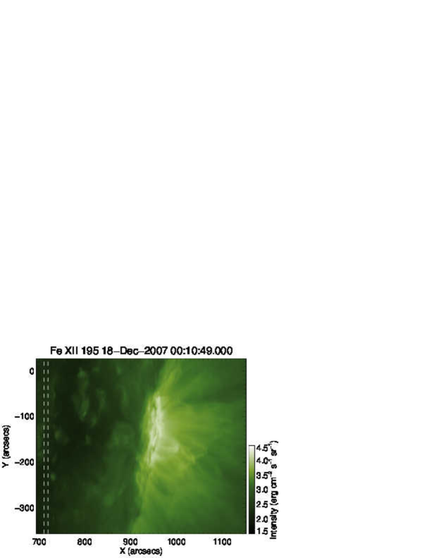
Fig. 4.16: Intensity image of Fe xii $195.12$Å taken by a raster scan at the west limb on 2007 December 18. The region between two vertical dashed lines indicates the location where the spectrum tilts were investigated.

We chose the region to be analyzed where (1) away from the active region on the limb as far as possible, and (2) less coronal bright points along all $y$ positions in the FOV. The best region satisfying those criteria was between two vertical dashed lines in Fig. 4.16. Here we show the variation of four line centroids from both SW and LW CCDs in Fig. 4.17: Fe viii $194.66$Å (upper left) and Fe x $184.54$Å (upper right) from the SW CCD, Si vii $275.35$Å (lower left) and Fe x $257.26$Å (lower right) from the LW CCD. Gray, red, and blue solid line respectively indicate the tilt given by Kamio et al. (2010), second order polynomial fitting, and third order polynomial fitting. The calibration given by Kamio et al. (2010) is shifted in each panel so that the value at the left vertical axis coincides with the second order polynomial fitting. A vertical bar in the right lower corner in each panel shows the velocity scale of $5\,\mathrm{km}\,\mathrm{s}^{-1}$. Note that Fe viii and Si vii emission lines have similar formation temperature of $\log T\,[\mathrm{K}]\simeq 5.7$–$5.8$.

The curve given by Kamio et al. (2010) represents the behavior of line centroids quite well in the SW CCD as seen in two upper panel in Fig. 4.17. Data points are a little more dispersed in lower panels because of the less number of photons of those emission lines, nevertheless, the curve given by Kamio et al. (2010) again represents their behavior. Therefore we adopt the calibration given by Kamio et al. (2010) in this chapter.

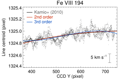
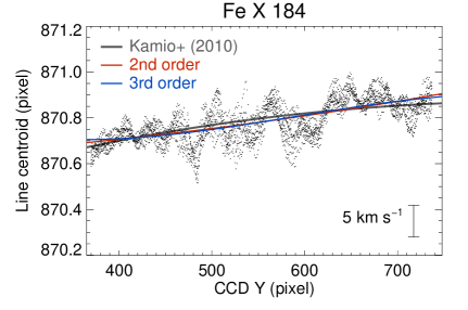
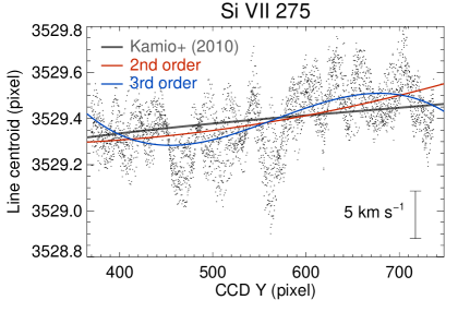
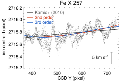
Fig. 4.17: The spectrum tilts for Fe viii $194.66$Å, Si vii $275.35$Å, and Fe x $184.54$Å/$257.26$Å. Gray, red, and blue solid line respectively indicate the tilt given by Kamio et al. (2010), second order polynomial fitting, and third order polynomial fitting. A vertical bar in the right lower corner in each panel shows the velocity scale of $5\,\mathrm{km}\,\mathrm{s}^{-1}$.

Appendix 4.B Mg emission lines

At the active region core, Mg vii $278.40$Å exhibited Doppler velocity of $\simeq-15\,\mathrm{km}\,\mathrm{s}^{-1}$. Here Fig. 4.18 shows line profiles of the emission line. The line profile at the core region (green) has a distinct uplift of the spectrum at $\lambda=278.20$–$278.30$Å which is considered to be P xii $278.29$Å ($\log T\,[\mathrm{K}]=6.3$). This could cause the apparent blueshift of Mg vii.

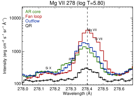
Fig. 4.18: Line profiles of Mg vii $278.40$Å at the quiet region (black), the outflow region (blue), fan loop (red), and the core region (green). A vertical dashed line in each panel indicates a line centroid of the emission line at the quiet region.

Appendix 4.C Temperature dependence of the Doppler velocities (all samples)

The temperature dependence of the Doppler velocities for all white boxes indicated in Fig. 4.5 is shown here. Fig. 4.19–4.21 respectively show the result for core regions (C1–C3), outflow regions (U1–U4), and fan loops (F1–F4).

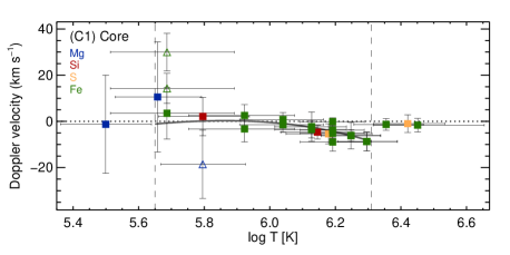
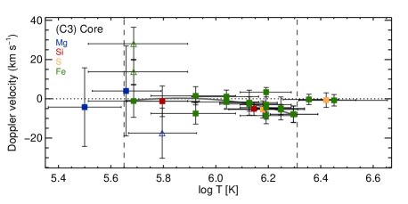
Fig. 4.19: Temperature dependence of the average Doppler velocities in C1–C3 indicated by white boxes in Fig. 4.5.

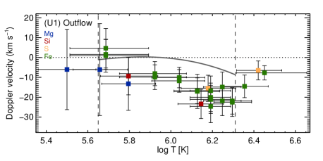
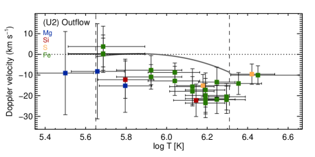
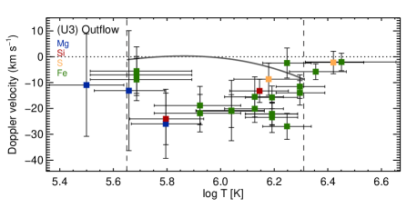
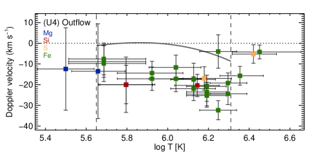
Fig. 4.20: Temperature dependence of the average Doppler velocities in U1–U4 indicated by white boxes in Fig. 4.5.

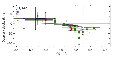
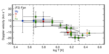
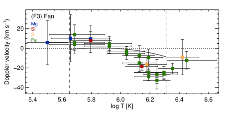
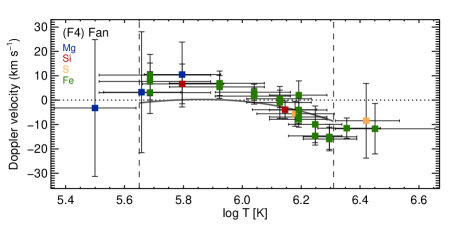
Fig. 4.21: Temperature dependence of the average Doppler velocities in F1–F4 indicated by white boxes in Fig. 4.5.

Appendix 4.D Residual from single Gaussian fitting in the outflow region

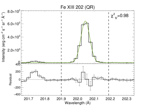
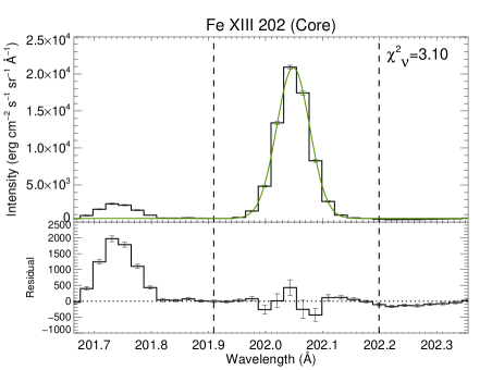
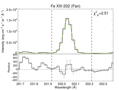
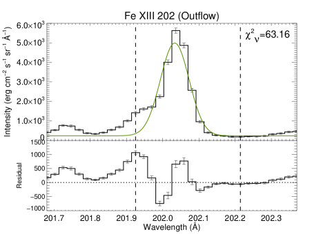
Fig. 4.22: Line profiles of Fe xiii $202.04$Å and their residual from a single Gaussian. Upper left: the quiet region. Upper right: the active region core. Lower left: fan loop. Lower right: the outflow region.

In order to look into the deviation from symmetric profile at the outflow region, we show four line profiles of Fe xiii $202.04$Å in Fig. 4.22. This emission line exhibited the most significant enhancement of its blue wing in the outflow region. Fig. 4.22 shows the line profile in the upper part and the residual from a single Gaussian in the lower part in each panel. A green line plotted over on the spectrum in each panel indicates a single Gaussian fitted to it. An emission line at around $\lambda=201.7$–$201.8$Å is Fe xi $201.73$Å, which is weaker than Fe xiii $202.04$Å in any regions. It is confirmed that the line profiles in the quiet region, the core region, and a fan loop are well represented by a single Gaussian as seen in the residuals. On the other hand, the line profile in the outflow region significantly deviates from a single Gaussian, and the deviation crudely reaches up to $1000/1.5\times 10^{4}\simeq 0.07=7$% in the peak of major component. The deviation from the single Gaussian can be evaluated quantitatively by the reduced chi square $\chi^{2}_{\nu}=\Sigma_{i}\left[\phi(\lambda_{i})-y_{\mathrm{fit}}(\lambda_{i})\right]^{2}/\nu$, where $\phi(\lambda_{i})$ is the spectral intensity at $\lambda=\lambda_{i}$, $y_{\mathrm{fit}}(\lambda)$ is the fitted Gaussian, and $\nu$ is the number of degrees of freedom. The value of $\chi^{2}_{\nu}$ was written beside the fitted range indicated by two vertical dashed lines.

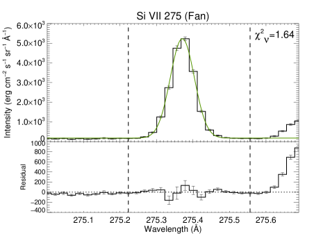
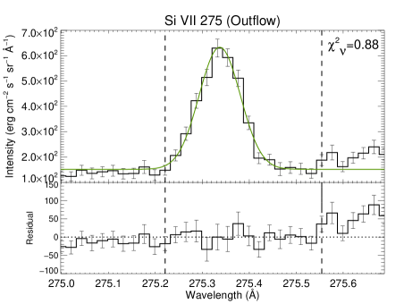
Fig. 4.23: Line profiles of Si vii $275.35$Å ($\log T\,[\mathrm{K}]=5.80$) and their residual from a single Gaussian. Left: in a fan loop. Right: in the outflow region.

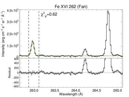
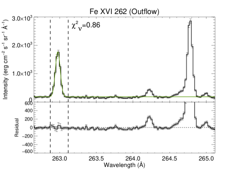
Fig. 4.24: Line profiles of Fe xvi $262.98$Å ($\log T\,[\mathrm{K}]=6.45$) and their residual from a single Gaussian. Left: in a fan loop. Right: in the outflow region.

As an example of a line profile from the temperature below $\log T\,[\mathrm{K}]=6.0$, those of Si vii $275.35$Å ($\log T\,[\mathrm{K}]=5.80$) are shown in Fig. 4.23. In contrast to Fe xiii, this transition region emission line shows almost no significant deviations from a single Gaussian. There might be a little excess in the line profile in the outflow region around $275.27$Å, but since it is only a single pixel, it could be better not to think this excess as significant. As inferred in Section 4.3.4, the hottest emission line analyzed here, Fe xvi $262.98$Å ($\log T\,[\mathrm{K}]=6.45$) neither did not have significant deviations from a single Gaussian as shown in Fig. 4.24.

The temperature dependence of $\chi^{2}_{\nu}$ for the temperature range of $\log T\,[\mathrm{K}]=5.5-6.5$ is shown in Fig. 4.25. It is clearly shown that Fe xii–xv exhibit largest $\chi^{2}_{\nu}$. The transition region lines (Mg v–vii, Si vii, etc.) and two hot emission lines (S xiii and Fe xvi) indicate much less $\chi^{2}_{\nu}$ of the order of unity as expected from Fig. 4.23 and 4.24. The deviations for Fe xii–xv are caused by the existence of enhanced blue wing, and this plot shows that the enhanced blue wings are distributed around the temperature of $\log T\,[\mathrm{K}]=6.2-6.3$. Note that the number of fitted bins is not the same for the emission lines so that we could not directly interpret this plot as a significance probability.

Fig. 4.25: $\chi^{2}_{\nu}$ of the single-Gaussian fitting for emission lines within the temperature range of $\log T\,[\mathrm{K}]=5.5\text{--}6.5$.

Chapter 5 Density of the upflows

5.1 Introduction

Although a number of observations have revealed the physical properties such as the source region and velocity of the outflows from the edge of active regions, there is one remained missing property: the electron density of the outflow itself. The density of an outflow region derived by using the line ratio of Fe xii $186.88$Å/$195.12$Å was $\simeq 7\times 10^{8}\,\mathrm{cm}^{-3}$ (Doschek et al. 2008), which is slightly lower than the typical value in active region ($n_{\mathrm{e}}\geq 10^{9}\,\mathrm{cm}$). Recently, Brooks & Warren (2012) carried out differential emission measure (DEM) analysis at the outflow regions. It was revealed that the properties of DEM and also the chemical abundance are rather close to those of active region, from which the authors concluded that the outflowing plasma originate in the active region loops. The interchange reconnection was considered to be a candidate for accelerating the plasma into the outer atmosphere (Baker et al. 2009).

The electron density of the outflow itself should help us to better understand the nature of the outflows, however, there has been no such challenge until present. One point of view is that those outflows are directly linked to the coronal heating in a way which the outflowing plasma fills the outer atmosphere and form the corona (De Pontieu et al. 2009; McIntosh et al. 2012). The impulsive heating in a coronal loop induces an upflow from its footpoint, which is a possible candidate what we see as the outflow (Del Zanna 2008; Hara et al. 2008). Outflows can be also caused by the sudden change of the pressure environment in a coronal loop (Bradshaw et al. 2011).

The analytical approach was recently proposed in terms of the ratio of the electron density between major rest component ($n_{\mathrm{Major}}$) and minor outflow component (enhanced blue wing, $n_{\mathrm{EBW}}$) in coronal emission line profiles (Klimchuk 2012). It was shown that if the tips of the chromospheric spicules supply the coronal plasma (De Pontieu et al. 2011), that ratio (here after denoted as $n_{\mathrm{EBW}}/n_{\mathrm{Major}}$) takes a value of an order of $10$–$100$, while tiny impulsive heating (i.e., nanoflare) creates the ratio of $0.4$–$1$ (Patsourakos & Klimchuk 2013). Thus, it was suggested that the ratio $n_{\mathrm{EBW}}/n_{\mathrm{Major}}$ can be used as a diagnostic tool which enables us to discriminate these two mechanisms in the corona.

Fig. 5.1: Theoretical line ratio calculated by CHIANTI database ver. 7 (Dere et al. 1997; Landi et al. 2012). (a) Fe xiv $264.78$Å/$274.20$Å. (b) Si vii $274.18$Å/$275.35$Å.

In this study, we used the spectroscopic data obtained with EIS onboard Hinode in order to measure the electron density of the outflows for the first time. As a line pair suitable for our purpose, Fe xiv $264.78$Å and $274.20$Å were chosen because (1) those emission lines have a distinct enhanced blue wing at the outflow region which leads to better signal-to-noise ratio, (2) they consist of relatively clean emission lines and their line wings in shorter wavelength side do not overlap with other emission lines, different from the cases for Fe xii $186.88$Å/$195.12$Å and Fe xiii $202.04$Å/$203.83$Å, and (3) the Fe xiv line pair is sensitive to the density range of $n_{\mathrm{e}}=10^{8\text{--}12}\,\mathrm{cm}^{-3}$, which is wider than other line pairs.

5.2 Observation and calibration

5.2.1 EIS raster scan

In this study, we analyzed a raster scan obtained with Hinode/EIS, which observed active region NOAA AR10978 (hereafter AR10978) at the center of the solar disk. Overall properties of the active region was described in the previous chapter. The scan with narrow $1^{\prime\prime}$ slit started on 2007 December 11 00:24:16UT and ended at 04:47:29UT. Field of view (FOV) was $256^{\prime\prime}\times 256^{\prime\prime}$ and exposure time was $60\,\mathrm{s}$. The EIS data was processed through the standard software which detects the cosmic ray hits on the CCD pixels, subtracts the dark current bias, and corrects DN at warm pixels. The DN is converted into the unit of intensity: $\mathrm{erg}\,\mathrm{cm}^{-2}\,\mathrm{s}^{-1}\,\mathrm{sr}^{-1}\,\text{\AA}^{-1}$. This quantity should be called as spectral intensity in the literature, however, we use a term intensity for the simplicity. One complicated point in the calibration is the thermal drift of the projected location on the CCD pixels due to the orbital motion of Hinode. Since the relative position of two emission lines Fe xiv $264.78$Å and $274.20$Å is the most important factor in this analysis, we roughly calibrated the wavelength through the method developed by Kamio et al. (2010).

5.2.2 Relative wavelength calibration

In order to make a precise fitting for Fe xiv $264.78$Å/$274.20$Å simultaneously, we have to know the wavelength positions of each emission line on the EIS spectrum which correspond to the same Doppler velocity. Considering the Doppler effect, centroids of Fe xiv $264.78$Å and $274.20$Å shift as

$$\lambda_{\mathrm{obs,}\,274}=\left(1+\frac{v_{\mathrm{LOS}}}{c}\right)\lambda_{0,\,274}$$ (5.1)

$$\lambda_{\mathrm{obs,}\,264}=\left(1+\frac{v_{\mathrm{LOS}}}{c}\right)\lambda_{0,\,264},$$ (5.2)

where $\lambda_{\mathrm{obs,}274}$ and $\lambda_{\mathrm{obs,}264}$ are observed centroids, $v_{\mathrm{LOS}}$ is line-of-sight velocity (positive means that the plasma move away from an observer), and $\lambda_{0,274}$ and $\lambda_{0,264}$ are the rest wavelength that we do not know. We can safely assume Doppler velocities in each equation have the same value because these two emission lines are radiated from the same degree of Fe ions. Dividing Eq. (5.1) by Eq. (5.2) leads to

$$\frac{\lambda_{\mathrm{obs,}\,274}}{\lambda_{\mathrm{obs,}\,264}}=\frac{\lambda_{0,\,274}}{\lambda_{0,\,264}}.$$ (5.3)

This equation means that the ratio of the centroid wavelengths in two emission lines becomes constant independent of the Doppler velocity of the emitting plasma. Once we obtain the constant $\lambda_{0,\,274}/\lambda_{0,\,264}$, it is possible to determine wavelength positions of the two emission lines corresponding to the same Doppler velocity without absolute calibration of the zero-velocity point.

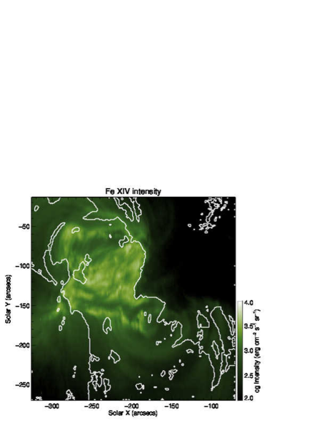
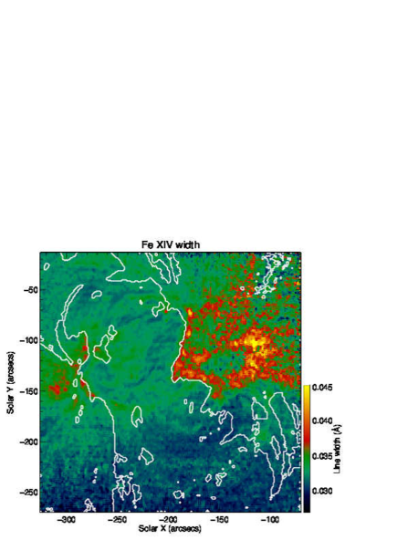
Fig. 5.2: Left: map of Fe xiv $264.78$Å intensity on 2007 December 11. Right: map of Fe xiv $264.78$Å line width. White contours indicate the boundary of the area excluded when making the histogram of the ratio $\lambda_{\mathrm{obs,}274}/\lambda_{\mathrm{obs,}264}$.

In order to determine the constant $\lambda_{0,\,274}/\lambda_{0,\,264}$ in Eq. (5.3), we obtained the centroids $\lambda_{\mathrm{obs,}\,274}$ and $\lambda_{\mathrm{obs,}\,264}$ from the EIS scan. We excluded the region where (1) line blend is significant, (2) the intensity is low, or (3) line profiles of Fe xiv obviously deviate from single Gaussian. There is a weak Si vii 274.18Å emission line near Fe xiv $274.20$Å, separated by roughly one EIS spectral pixel. This may cause spurious blueshift of Fe xiv $274.20$Å. When considering the extreme example, if Si vii 274.18Å has the same intensity as Fe xiv $274.20$Å, the fitted centroid becomes 274.19Å (i.e., mean of the two emission lines), which means a blueshift of $\sim 10\,\mathrm{km}\,\mathrm{s}^{-1}$. To avoid this spurious effect, we excluded the pixel for the intensity ratio Si vii $275.35$Å/Fe xiv $264.78$Å exceed 0.1, which might produce the spurious blueshift of $\sim 0.5\,\mathrm{km}\,\mathrm{s}^{-1}$ in the maximum. Secondly, the region where the intensity of Fe xiv $264.78$Å is lower than $1500\,\mathrm{erg}\,\mathrm{cm}^{-2}\,\mathrm{s}^{-1}\,\mathrm{sr}^{-1}$ was excluded to reduce the uncertainty in determining the value of Eq. (5.3). Thirdly, we should exclude the area where the line profile significantly deviates from single Gaussian.

The boundary of excluded area is shown by white contours in Fig. 5.2. Only the active region core between the two white contours was used as seen from the map of Fe xiv intensity (the left panel). The right panel shows the map of line width, from which we can see that the outflow region was also excluded where the line profiles skews and have long tail in the shorter wavelength which produces enhanced line width when fitted by single Gaussian.

Fig. 5.3 shows the histogram of the ratio $\lambda_{\mathrm{obs,}274}/\lambda_{\mathrm{obs,}264}$ after excluding the area describe above. The average value ($\alpha$) was $\alpha=1.0355657$ and its standard deviation was $4.4\times 10^{-6}$. We also derived the ratio $\lambda_{\mathrm{obs,}\,274}/\lambda_{\mathrm{obs,}\,264}$ from another scan data in the same day (but different time; 10:25:42UT), which resulted in the exactly same average value but slightly larger standard deviation of $5.4\times 10^{-6}$ which might came from the shorter exposure time ($40\,\mathrm{s}$). Note that the theoretical ratio predicted by CHIANTI is $1.0355559$ and it is within the deviation coming from the precision of the wavelength calibration for the EIS long wavelength band ($\simeq 0.002$Å; Brown et al. 2007). We used the obtained $\alpha$ to fit the two emission lines from Fe xiv $264.78$Å/$274.20$Å simultaneously, and to confirm the results by exploiting a new method ($\lambda$-$n_{\mathrm{e}}$ diagram) in Chapter 6.

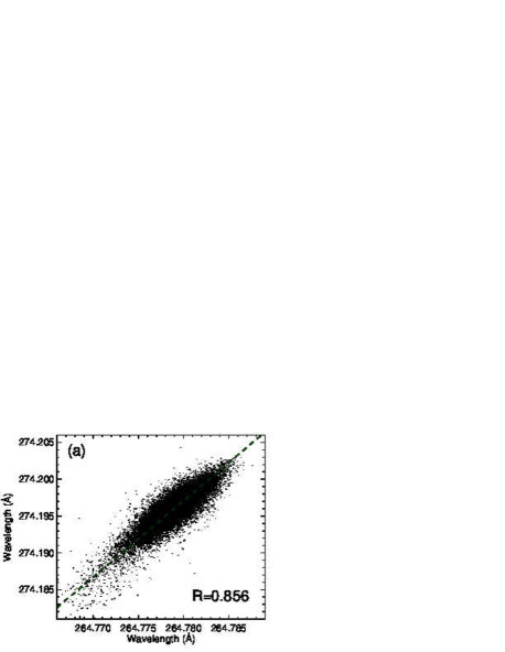
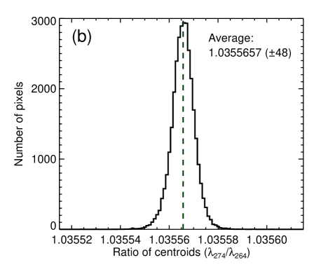
Fig. 5.3: Histogram of the ratio of centroids for two emission lines Fe xiv 274.20/264.78 in the raster scan taken on 2007 December 11. Vertical dashed line indicates the average value ($1.0355657\pm 0.0000044$).

5.3 Density diagnostics of upflows

One of main achievements in this thesis is the density measurement of the outflow from the edge of an active region for the first time. Previous observations have revealed that the density of the outflow region measured by using a line pair Fe xii $186.88$Å/$195.12$Å indicates $7\times 10^{8}\,\mathrm{cm}^{-3}$ which is close to that of coronal holes rather than that of active regions (Doschek et al. 2008). However, density of the outflow itself, to be measured by separating its component from the major component in line profiles, has not been investigated so far.

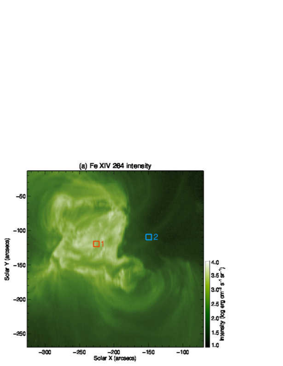
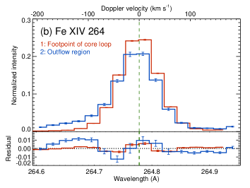
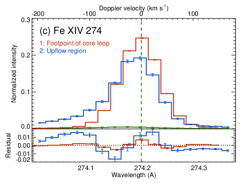
Fig. 5.4: Line profiles of the active region AR10978. (a) Context image of AR10978 obtained on 2007 December 11 00:24:16–04:47:29UT. Intensity of Fe xiv $264.78$Å is shown. Boxes numbered as 1 (red) and 2 (blue) respectively indicate a footpoint of core loops and the outflow region. (b) Fe xiv $264.78$Å spectra. (c) Fe xiv $274.20$Å spectra. In each panel, line profiles at the footpoint of core loops (red histogram) and at the outflow region analyzed here (blue histogram) are shown in the upper half. The spectra were normalized by their integration. Residuals from the single-Gaussian fitting of each histogram are shown in the lower half. Green histogram in panel (c) shows estimated spectrum of Si vii $274.18$Å.

There are three reasons of the difficulties in the analysis of spectroscopic data obtained by Hinode/EIS. Firstly, the signals from an upflow are detected as an enhanced blue wing (hereafter, EBW) component in emission line profiles. Examples of them are shown in Fig. 5.4. In each panel, line profiles at the footpoint of a core loop (red histogram) and at the outflow region analyzed here (blue histogram) are shown in the upper half. Residuals from single-Gaussian fitting of each histogram are shown in the lower half, which is quite useful in detecting weak signals in line wing (Hara et al. 2008). There is a significant enhancement at the blue wing ($\leq-100\,\mathrm{km}\,\mathrm{s}^{-1}$) both in Fe XIV $264.78$Å and $274.20$Å as shown by blue histograms. Green histogram in panel (c) shows estimated spectrum of Si vii $274.18$Å which was subtracted in the density diagnostics described later. The EBW component is weak in most cases as seen in spectra indicated by blue histograms shown in Fig. 5.4. In addition, EBW component is significantly dominated by the strong component almost at rest, which makes the analysis of upflows quite uncertain.

Secondly, the density measurement of the outflow itself needs the accurate determination of the rest wavelengths of emission lines from which we fit the two emission lines simultaneously and deduce the intensity. As described earlier in this thesis, this is often laborious because we do not have the absolute measure of the wavelength corresponding to each observational spectral pixels.

Thirdly, density measurement needs at least two emission lines from the same ion (e.g., Fe xiv as used in this thesis). This means that the two emission lines should be fitted simultaneously using same parameters such as Doppler velocity and line width. No previous studies on the outflows from the edge of active region have dealt with such fitting.

Procedure of density diagnostics in this thesis is as follows: (1) integration of neighboring multiple pixels in order to reduce the noise, (2) determination of the wavelength position corresponding to the same Doppler velocity, (3) removal of blending Si vii $274.18$Å from Fe xiv $274.20$Å using Si vii $275.35$Å as a reference, (4) simultaneous fitting of Fe xiv $264.78$Å and $274.20$Å, and (5) density inversion using a theoretical curve from CHIANTI as a function of the intensity ratio. In following sections, each procedure will be described in detail.

5.3.1 Integration of observational pixels

The outflows from the edge of active regions are usually detected as an EBW in emission line profiles. Its intensity does not exceed $\sim 25\mathrm{\%}$ of that of the major component (Doschek 2012). This makes the analysis difficult since the photon noise of the major component affects the emission from EBW. In addition, the region where the outflows can be seen is usually dark (i.e., small signal-to-noise ratio). In order to improve the signal-to-noise ratio, we integrated over multiple observational pixels in space using a square box with the size of $5^{\prime\prime}\times 5^{\prime\prime}$. Larger size of the integration box generally results in better signal-to-noise ratio, however, we chose the size of integration box so as not to lose the information of the outflow region. In the integration, the pixels with instrumental problems (i.e., hot or bad pixels) were excluded.

5.3.2 De-blending of Si vii from Fe xiv 274.20Å

We should subtract blended lines from both Fe xiv lines. Fe xiv $264.78$Å is isolated without significant contributions from other emission lines. As for Fe xvi $265.01$Å, it is far enough from Fe xiv $264.78$Å in non-flare situation. Moreover, estimated peak intensity of Fe xvi $265.01$Å was around $100\,\mathrm{erg}\,\mathrm{cm}^{-2}\,\mathrm{s}^{-1}\,\mathrm{sr}^{-1}\,\text{\AA}^{-1}$ in the observed outflow region, which is at most the background level of Fe xiv $264.78$Å as seen in Fig. 5.5.

On the other hand, Fe xiv 274.20 potentially has a contribution from Si vii $274.18$Å, which may become significant in the vicinity of an active region because Si vii emission often comes from the footpoint of cool loops extending from the edge of the active region. We should subtract this blend from Fe xiv $274.20$Å.

In this study, the spectrum of Si vii $274.18$Å was calculated by using the observed line profile of Si vii $275.35$Å which is known to be clean (i.e., without any significant blend). The intensity ratio of Si vii $274.18$Å/$275.35$Å is at most $0.25$ as calculated from CHIANTI version 7 (Dere et al. 1997; Landi et al. 2012). The value has a dependence in the density range $10^{8}\,\mathrm{cm}^{-3}\leq n_{\mathrm{e}}\leq 10^{10}\,\mathrm{cm}^{-3}$, and it varies $0.06$–$0.27$ (monotonically increasing) as shown in Fig. 5.1. First we remove the blending Si vii $274.18$Å for the case $n_{\mathrm{e}}=10^{9}\,\mathrm{cm}^{-3}$ (Si vii electron density), and after that we considered three cases of the ratio corresponding to the density of $10^{8}$, $10^{9}$, and $10^{10}\,\mathrm{cm}^{-3}$. In order to make our analysis be more robust, we excluded the location where the estimated intensity of Si vii $274.18$Å exceeds $5$% of the Fe xiv intensity. Using the theoretical ratio, the intensity of Si vii $275.35$Å was converted into that of Si vii $274.18$Å. The spectrum of Si vii $275.35$Å was then placed at Si vii $274.18$Å taking into account the shift of Si vii $275.35$Å from the rest wavelength using the relative difference between wavelength of Si vii $274.18$Å and $275.35$Å (i.e., $1.1808$Å) given by CHIANTI database. Note that since there were no locations where Si vii $274.18$Å dominates Fe xiv $274.20$Å in the data, we could not determine the relative wavelength position of the two Si vii lines, therefore we used the wavelength difference given by CHIANTI for the Si vii lines. The data points of the estimated Si vii $274.18$Å in the wavelength direction were interpolated into the data points of Fe xiv $274.20$Å by cubic spline. Thus, we removed the blended Si vii $274.18$Å from Fe xiv $274.20$Å.

5.3.3 Simultaneous fitting of the two Fe xiv emission lines

In order to make the fitting more robust, the two emission line profiles of Fe xiv $264.78$Å/$274.20$Å were fitted simultaneously. It is based on the consideration that the emission line profiles coming from the same ion species must have the same Doppler shift and the same Doppler width. As seen in Fig. 5.4, emission line profiles of Fe xiv $264.78$Å and $274.20$Å from the active region core (red histogram) are obviously symmetric, while those from the outflow region (blue histogram) have an EBW. This EBW did not exceed the major component at everywhere in the outflow region ($\leq 30$%). Previous observations have never shown such emission line profiles whose EBW dominates over the major component (Doschek 2012).

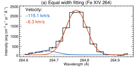
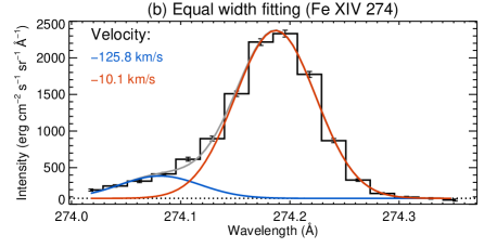
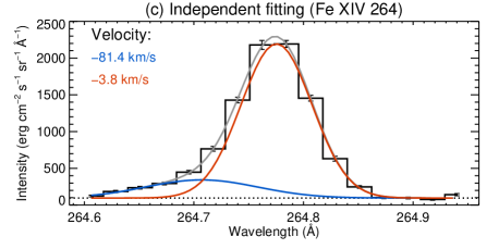
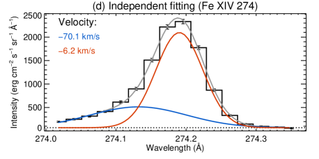
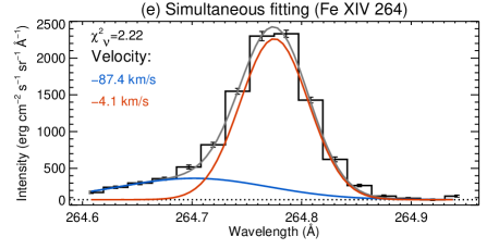
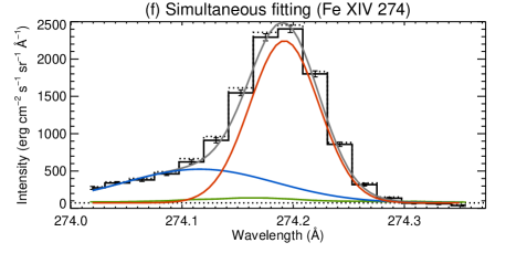
Fig. 5.5: Fitting results for Fe xiv $264.78$Å and $274.20$Å obtained by three different models. Upper row (panels a and b): fitting with double Gaussians those have the same line width applied to each line profile independently (model 1). Middle row (panels c and d): fitting with double Gaussians those do not necessarily have the same line width applied to each line profile independently (model 2). Lower row (panels e and f): fitting with double Gaussians applied to two line profiles simultaneously without the assumption of the same line width of two components (model 3).

In this study, the emission line profiles of the outflow region are assumed to be composed of two Gaussian components. Most of previous analysis on the outflows in the edge of an active region assumed that the main component and EBW have the same line width in order to reduce the possibility of approaching an unreasonable solution in the fitting parameter space, but the assumption could strongly affect the fitting (Bryans et al. 2010; Brooks & Warren 2012). Brooks & Warren (2012) mentioned that this assumption may cause the underestimation of the intensity of EBW. Line profile with EBW often shows rather longer tail in the line wing than that could be represented by a Gaussian which has the same line width as the major component. Moreover, the assumption that the major component and EBW have the same line width does not originate in the physical requirement.

In order to examine the differences in the fitting result between different constraint on the fitting parameters, we applied three fitting models to a line profile pair of Fe xiv $264.78$Å. Line centroid and line width are respectively denoted by $\lambda$ and $W$. The suffixes below represent: “1” for Fe xiv $264.78$Å, “2” for Fe xiv $274.20$Å followed by the component either “Major” or “EBW”. First model (model 1) assumes $W_{1,\mathrm{Major}}=W_{1,\mathrm{EBW}}$ and $W_{2,\mathrm{Major}}=W_{2,\mathrm{EBW}}$, and fits the line profiles of Fe xiv $264.78$Å and $274.20$Å separately with double Gaussians those have the same line width for each component. Second model (model 2) also fits the line profiles of the two Fe xiv separately, but with double Gaussians those do not necessarily have the same line width for each component. Third model (model 3) fits the two Fe xiv line profiles simultaneously by applying $\lambda_{2,\mathrm{Major}}=\alpha\lambda_{1,\mathrm{Major}}$, $\lambda_{2,\mathrm{EBW}}=\alpha\lambda_{1,\mathrm{EBW}}$ ($\alpha=1.0355657$; determined in Section 5.2.2), $W_{1,\mathrm{Major}}=W_{2,\mathrm{Major}}$, and $W_{1,\mathrm{EBW}}=W_{2,\mathrm{EBW}}$. We adopted model 3 for the electron density measurement in this study because it is physically most reasonable in the sense that the model deals the parameters (line centroids and thermal widths) consistently for both emission lines and does not impose the artificial restriction on the line widths.

The results for those three models are shown in Fig. 5.5. We obtained smaller and more blueshifted second component (EBW) with the model 1 in panels (a) and (b), which confirms the suggestion in Brooks & Warren (2012). In contrast, larger and less blueshifted EBWs were obtained with the models 2 and 3 as clearly seen in panel (c)–(f). In addition to this, the line widths of EBW component was much broader for the models 2 and 3 than for the model 1. It is not clear at present whether the increased widths may indicate superposition of multiple upflow components, which will be another point to be revealed in the future. The comparison between those three models shows that the results in previous analysis should underestimate the intensity of EBW with an artificial assumption that two components in line profile have the same line width. Moreover, independent fitting applied to two emission lines causes a discrepancy as seen in panel (c) and (d). The Doppler velocity of EBW component was $-81.4\,\mathrm{km}\,\mathrm{s}^{-1}$ for Fe xiv $264.78$Å while $-70.1\,\mathrm{km}\,\mathrm{s}^{-1}$ for Fe xiv $274.20$Å. Note that the rest wavelengths were determined from a limb observation on 2007 December 6, so these Doppler velocities have an uncertainty of $10\,\mathrm{km}\,\mathrm{s}^{-1}$ at most.

5.3.4 Density inversion

Now the densities of EBW and the major component can be obtained by referring to the theoretical intensity ratio of Fe xiv $264.78$Å/$274.20$Å as a function of electron density shown in Fig. 5.1. The intensity ratio monotonically increases within the density range of $10^{8}\,\mathrm{cm}^{-3}\leq n_{\mathrm{e}}\leq 10^{12}\,\mathrm{cm}^{-3}$. The electron density in the solar corona generally falls between $10^{8}\,\mathrm{cm}^{-3}$ (for coronal holes) and $10^{11}\,\mathrm{cm}^{-3}$ (for flare loops), so the intensity ratio of Fe xiv $264.78$Å/$274.20$Å is quite useful. The error in the density was calculated by using the 1-$\sigma$ error in the intensity ratio. The electron density is obtained from

$$n_{\mathrm{e}}=F^{-1}\left(\frac{I_{264}}{I_{274}}\right)\,\mathrm{,}$$ (5.4)

where $F^{-1}$ is the inverse function of the theoretical intensity ratio, and $I_{264}$ and $I_{274}$ are respectively the observed intensity of Fe xiv $264.78$Å and $274.20$Å. Using $\sigma_{I_{264}/I_{274}}$ as the error of observed intensity ratio, we estimate the error of the density $\sigma_{n_{\mathrm{e}}}$ as

$$n_{\mathrm{e}}\pm\sigma_{n_{\mathrm{e}}}=F^{-1}\left(\frac{I_{264}}{I_{274}}\pm\sigma_{I_{264}/I_{274}}\right)\,\mathrm{.}$$ (5.5)

The error $\sigma_{n_{\mathrm{e}}}$ was not dealt symmetrically in this definition, which comes from the fact the function $F$ has a curvature which can not be negligible compared to $\sigma_{I_{264}/I_{274}}$.

5.4 Density derived from Fe xiv 264.78Å/274.20Å

5.4.1 Results from single Gaussian fitting

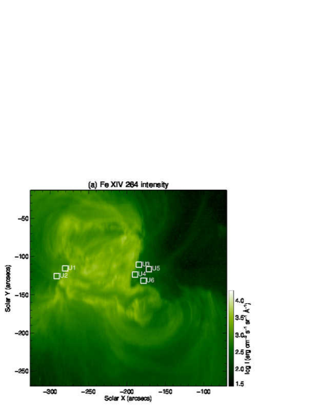
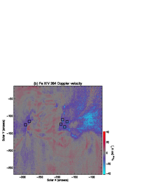
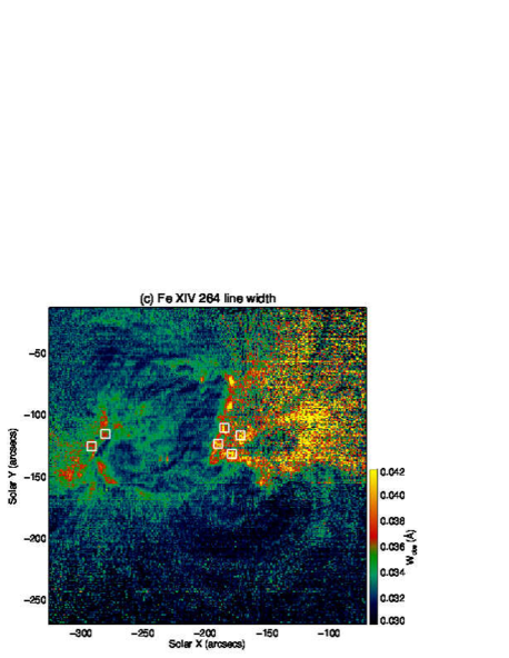
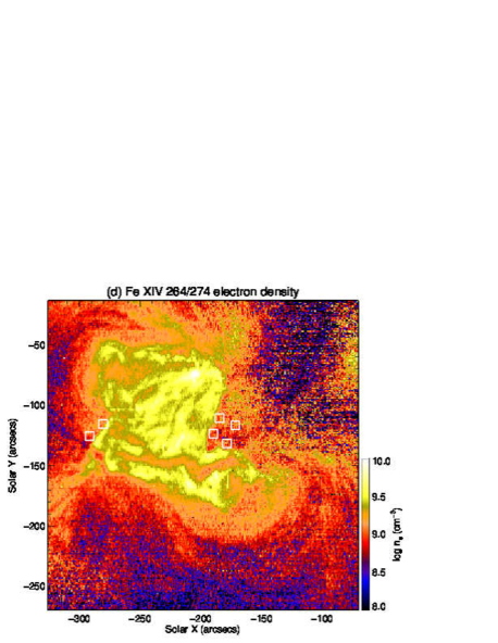
Fig. 5.6: Physical quantities deduced from single Gaussian fitting for Fe xiv $264.78$Å obtained on 2007 December 11 00:24:16–04:47:29UT. (a) Intensity of Fe xiv $264.78$Å. (b) Doppler velocity of Fe xiv $264.78$Å. (c) Line width of Fe xiv $264.78$Å. (d) Electron density derived from the line ratio Fe xiv $264.78$Å/$274.20$Å.

First we describe the results deduced from single-Gaussian fitting. As described above, line profiles at the outflow regions are known to have distorted shape which cannot be well represented by single Gaussian, nonetheless, the results deduced from single-Gaussian fitting may be useful because the fitting is much more robust in terms of the freedom of variables (e.g, 4 parameters for single Gaussian with constant background and 7 parameters for double Gaussians). Fig. 5.6 shows the map of intensity, Doppler velocity, line width of Fe xiv $264.78$Å, and electron density derived from the line ratio Fe xiv $264.78$Å/$274.20$Å. The blending Si vii $274.18$Å was taken into account and subtracted by referring to Si vii $275.35$Å. It is clear from panel (b) that there is the outflow regions (i.e., blueshift) at the east/west edge of the active region core around $(x,y)=(-260^{\prime\prime},-120^{\prime\prime})$ and $(-175^{\prime\prime},-125^{\prime\prime})$. Panel (c) shows that the line width at those outflow regions is larger than other locations by $\Delta W=0.020\text{--}0.027$Å (square root of the difference of squared line width) equivalent to $\delta v=20\text{--}30\,\mathrm{km}\,\mathrm{s}^{-1}$, which is similar to a result reported previously (Doschek et al. 2008; Hara et al. 2008). The electron density at the outflow regions is $n_{\mathrm{e}}=10^{8.5\text{--}9.5}\,\mathrm{cm}^{-3}$, which is lower than that at the core ($n_{\mathrm{e}}\geq 10^{9.5}\,\mathrm{cm}^{-3}$).

We selected the regions to be studied as similar way as that in Chapter 4. We defined the outflow regions as the locations (1) where the line width of Fe xiv $264.78$Å is enhanced, and (2) which can be separated from fan loops seen in Si vii intensity map though not shown here. The selected six regions are indicated by white boxes in each map (numbered by U1–U6 as written in panel (a), whose size is $8^{\prime\prime}\times 8^{\prime\prime}$. Those regions are located beside the bright core as seen in the intensity map (panel a). We hereafter refer U1–U2 as the eastern outflow region and U3–U6 as the western outflow region.

5.4.2 Density of the upflows

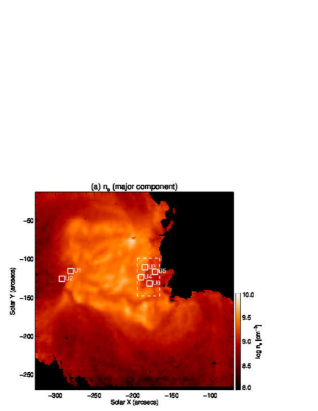
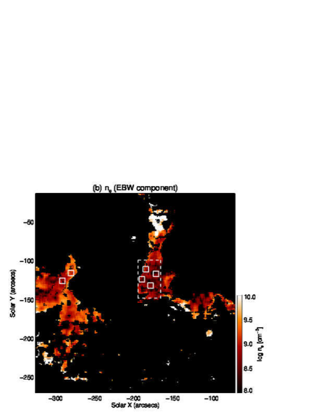
Fig. 5.7: Electron density map deduced from two Gaussian fitting of an emission line pair Fe xiv $264.78$Å/$274.20$Å obtained by the raster scan on 2007 December 11 00:24:16–04:47:29UT. (a) Electron density of the major component. (b) Electron density of EBW component. Same color contour are used in the two panels. Pixels where the peak intensity of the major component ($I_{\mathrm{Major}}$) did not exceed $2.0\times 10^{3}\,\mathrm{erg}\,\mathrm{cm}^{-2}\,\mathrm{s}^{-1}\,\mathrm{sr}^{-1}\,\text{\AA}^{-1}$ were masked by black. White boxes numbered U1–U6 are the same as those in Fig. 5.6. The white dashed box indicate the entire western outflow region.

The electron density of EBW component was measured through the analysis described in Section 5.3. Fig. 5.7 shows the distributions of electron density for the major component ($n_{\mathrm{Major}}$) in panel (a) and EBW component ($n_{\mathrm{EBW}}$) in panel (b). Pixels where the peak intensity of the major component ($I_{\mathrm{Major}}$) did not exceed $2.0\times 10^{3}\,\mathrm{erg}\,\mathrm{cm}^{-2}\,\mathrm{s}^{-1}\,\mathrm{sr}^{-1}\,\text{\AA}^{-1}$ were masked by black. This threshold was determined by using the scatter plot of intensity and electron density of the major component shown in Appendix 5.B. Pixels falling into the next three conditions were displayed, and others were masked by black. (1) $I_{\mathrm{Major}}\geq 2.0\times 10^{3}\,\mathrm{erg}\,\mathrm{cm}^{-2}\,\mathrm{s}^{-1}\,\mathrm{sr}^{-1}\,\text{\AA}^{-1}$. (2) The intensity of EBW component ($I_{\mathrm{EBW}}$) exceeds $3$% of that of the major component ($I_{\mathrm{EBW}}/I_{\mathrm{Major}}\geq 0.03$). (3) The difference between the Doppler velocity of EBW component ($v_{\mathrm{EBW}}$) and that of the major component ($v_{\mathrm{Major}}$) satisfies $v_{\mathrm{EBW}}-v_{\mathrm{Major}}<-30\,\mathrm{km}\,\mathrm{s}^{-1}$ (i.e., the two components are well separated).

The relationship of electron density between the major component and EBW component are shown in Fig. 5.8. Scatter plot in panel (a) shows the electron density for the outflow regions U1–U6 (colored symbols) and for the entire western outflow region indicated by the white dashed box in Fig. 5.7 (black dots). The eastern outflow regions (U1–U2) and west ones (U3–U6) exhibit different characteristics. The scatter plots for U1–U2 indicate $n_{\mathrm{Major}}\leq n_{\mathrm{EBW}}$, while those for U3–U6 indicate $n_{\mathrm{Major}}\geq n_{\mathrm{EBW}}$. Panels (b) and (c) show the same data but in histograms for which colors again indicate the selected outflow regions. The gray (the major component) and turquoise (EBW component) histograms in the background of panel (c) are made for the entire western outflow region. Those two histograms clearly indicate that $n_{\mathrm{EBW}}$ ($10^{8.61\pm 0.24}\,\mathrm{cm}^{-3}$) is smaller than $n_{\mathrm{Major}}$ ($10^{9.18\pm 0.13}\,\mathrm{cm}^{-3}$) at the entire western outflow region, which confirms that our selection of the studied regions was not arbitrary. The average electron densities in each studied region are listed in Table 5.1.

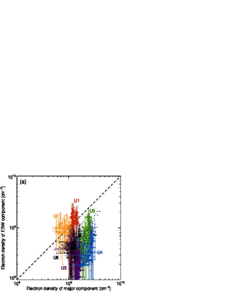
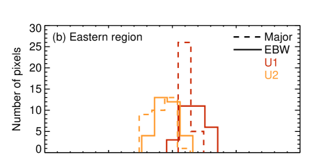
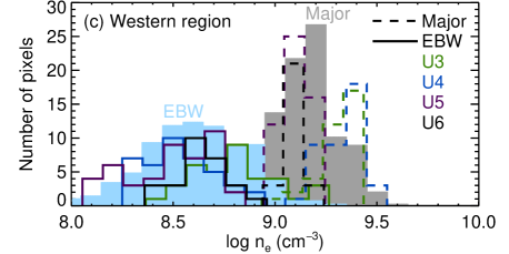
Fig. 5.8: (a) Scatter plot for Fe xiv electron density of the major component vs. that of EBW component. Colors indicate the selected region indicated by white boxes in Fig. 5.6. Triangles (Diamonds) represent the data points in the eastern (western) outflow regions. Numbers beside data points correspond to the name of the white boxes. Black dots show the electron density for the western outflow region indicated by a white dashed box in Fig. 5.7. The dashed line indicates point where two densities equal each other. (b) Histograms for the electron density of the major component (dotted) and EBW component (solid) in the eastern outflow region. (c) Histograms for the electron density of the major component (dotted) and EBW component (solid) in the western outflow region. The gray (the major component) and turquoise (EBW component) histograms in the background are made for the entire western outflow region. Those two histograms are multiplied by $0.1$.

5.4.3 Column depth

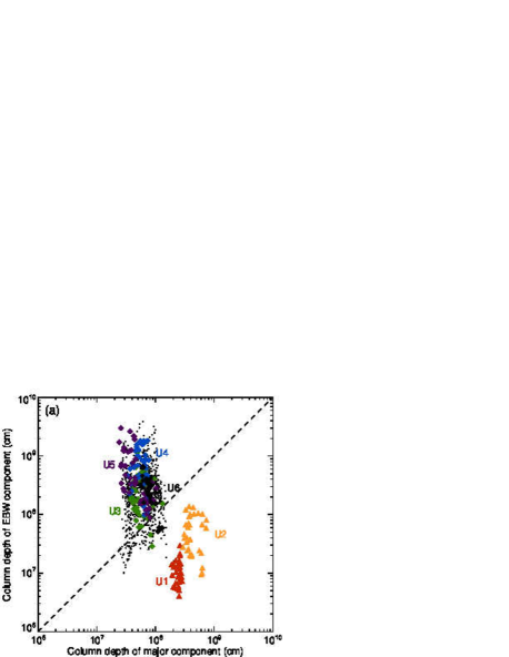
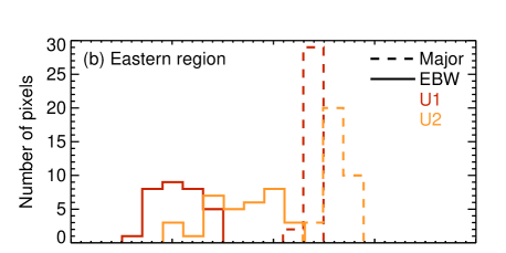
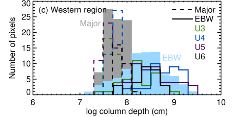
Fig. 5.9: (a) Scatter plot for column depth of the major component vs. that of EBW component. Colors indicate the selected region indicated by white boxes in Fig. 5.6. Triangles (Diamonds) represent the data points in the eastern (western) outflow regions. Numbers beside data points correspond to the name of the white boxes. Black dots show the column depth for the entire western region indicated by a white dashed box in Fig. 5.7. The dashed line indicates point where two quantities equal each other. (b) Histograms for column depth of the major component (dotted) and EBW component (solid) in the eastern outflow region. (c) Histograms for column depth of the major component (dotted) and EBW component (solid) in the western outflow region. The gray (the major component) and turquoise (EBW component) histograms in the background are made for the entire western outflow region. Those two histograms are multiplied by $0.1$.

Using the obtained electron density for each component in Fe xiv line profiles, the column depth of each component can be respectively calculated. We use the equation for the column depth including the filling factor,

$$h^{\ast}=hf=\dfrac{I}{n_{\mathrm{e}}^{2}G(n_{\mathrm{e}},\,T)}\,\text{,}$$ (5.6)

where $f$ is the filling factor, $I$ is the intensity of an emission line, $n_{\mathrm{e}}$ is the electron density, and $G(n_{\mathrm{e}},\,T)$ is the contribution function of an emission line. The quantity $h^{\ast}$ has a physical meaning as the plasma volume per unit area along the line of sight. Here the temperature substituted to Eq. (5.6) was simply assumed to take a single value $T_{\mathrm{f}}$ at which the contribution function $G(n_{\mathrm{e}},\,T)$ becomes maximum ($\log T_{\mathrm{f}}\,[\mathrm{K}]=6.30$ for the Fe xiv lines used here). Panel (a) in Fig. 5.9 shows a scatter plot for the column depth of the major component ($h_{\mathrm{Major}}$) and that of EBW component ($h_{\mathrm{EBW}}$). Colored symbols respectively indicate the studied regions (U1–U2 for the eastern outflow region, and U3–U6 for the western outflow region). As similar to the result for the electron density, the eastern and western outflow regions exhibit different characteristics: $h_{\mathrm{Major}}\geq h_{\mathrm{EBW}}$ in the eastern region, and $h_{\mathrm{Major}}\leq h_{\mathrm{EBW}}$ in the western region. Panels (b) and (c) display the same data in the form of histogram respectively for the eastern and western outflow region. The gray and turquoise histograms in the background of panel (c) show the results for the entire western outflow region indicated by a white dashed box in Fig. 5.7. Table 5.1 shows the column depths averaged in each studied region.

The result $h_{\mathrm{Major}}\leq h_{\mathrm{EBW}}$ in the western outflow regions (U3–U6) means that the upflow dominates over the rest component in terms of the volume, opposite to the composition ratio of emission line profile itself. The value of $h_{\mathrm{EBW}}\simeq 10^{8.0\text{--}9.0}\,\mathrm{cm}$ can be understood by considering that the inclination of the magnetic field lines in the western outflow region was $30^{\circ}\text{--}50^{\circ}$ and the horizontal spatial scale of the region was the order of $10^{\prime\prime}(\sim 10^{9}\,\mathrm{cm})$, which leads to the vertical height of nearly the same amount. On the other hand, it is clearly indicated that $h_{\mathrm{EBW}}$ is smaller than $h_{\mathrm{Major}}$ by up to one order of magnitude in the eastern outflow region (U1–U2). This means that the upflows possess only a small fraction compared to the rest plasma.

5.4.4 Uncertainty in Si vii density

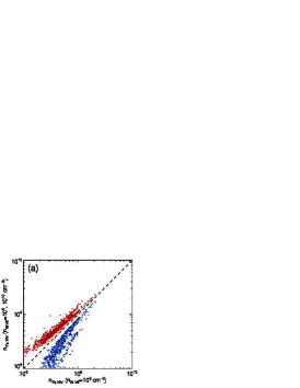
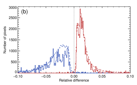
Fig. 5.10: (a) Scatter plots of derived Fe xiv density ($n_{\mathrm{Fe\textsc{xiv}}}$) for different electron density of Si vii ($n_{\mathrm{Si\textsc{vii}}}$). Horizontal axis indicates $n_{\mathrm{Fe\textsc{xiv}}}$ of EBW component derived by assuming $n_{\mathrm{Si\textsc{vii}}}=10^{9}\,\mathrm{cm}^{-3}$. Vertical axis indicates $n_{\mathrm{Fe\textsc{xiv}}}$ of EBW component derived by assuming $n_{\mathrm{Si\textsc{vii}}}=10^{8}\,\mathrm{cm}^{-3}$ (blue) and $10^{10}\,\mathrm{cm}^{-3}$ (red). (b) The same data as in panel (a) but the horizontal axis indicates a relative difference $\Delta n_{\mathrm{Fe\textsc{xiv}}}/n_{\mathrm{Fe\textsc{xiv}}}$, where $\Delta n_{\mathrm{Fe\textsc{xiv}}}$ is a difference of $n_{\mathrm{Fe\textsc{xiv}}}$ for different $n_{\mathrm{Si\textsc{vii}}}$ ($10^{8}$ and $10^{10}\,\mathrm{cm}^{-1}$) measured from the case for $n_{\mathrm{Si\textsc{vii}}}=10^{9}\,\mathrm{cm}^{-3}$.

In the line profile analysis, we assumed that the electron density corresponding to the temperature of Si vii (i.e., the transition region; hereafter $n_{\mathrm{Si\textsc{vii}}}$) was $10^{9}\,\mathrm{cm}^{-3}$. Since the electron density is not the same for emission lines with different formation temperature, there is an uncertainty in $n_{\mathrm{Si\textsc{vii}}}$ which cannot be determined from the data used in this analysis. In order to evaluate the error in the electron density derived for Fe xiv ($n_{\mathrm{Fe\textsc{xiv}}}$) coming from this uncertainty, we remove the blending Si vii at Fe xiv $274.20$Å in three cases for $n_{\mathrm{Si\textsc{vii}}}$: $10^{8}$, $10^{9}$, and $10^{10}\,\mathrm{cm}^{-3}$, and derived $n_{\mathrm{Fe\textsc{xiv}}}$ for each case. Panel (a) in Fig. 5.10 shows scatter plots for the electron density of EBW component within the entire western outflow region derived for the case $n_{\mathrm{Si\textsc{vii}}}=10^{9}\,\mathrm{cm}^{-3}$ vs. $10^{8}\,\mathrm{cm}^{-3}$ $(10^{10}\,\mathrm{cm}^{-3})$ by blue (red). The $n_{\mathrm{Fe\textsc{xiv}}}$ of EBW component derived by assuming $n_{\mathrm{Si\textsc{vii}}}=10^{8}$ $(10^{10})\,\mathrm{cm}^{-3}$ becomes smaller (larger). Panel (b) in Fig. 5.10 shows those relative differences $\Delta n_{\mathrm{Fe\textsc{xiv}}}/n_{\mathrm{Fe\textsc{xiv}}}$, where $\Delta n_{\mathrm{Fe\textsc{xiv}}}$ is a difference of $n_{\mathrm{Fe\textsc{xiv}}}$ for different $n_{\mathrm{Si\textsc{vii}}}$ ($10^{8}$ and $10^{10}\,\mathrm{cm}^{-1}$) measured from the case for $n_{\mathrm{Si\textsc{vii}}}=10^{9}\,\mathrm{cm}^{-3}$. Colors (red and blue) indicate the same meaning as in panel (a). Solid and Dashed histograms respectively indicate that for the western outflow region (the white dashed box in Fig. 5.7) and for the entire field of view. These relative differences were calculated in log scale. The histograms show that the error coming from the difference of $n_{\mathrm{Si\textsc{vii}}}$ does not exceed $5$%. It means that the error is around $10^{0.4\text{--}0.5}$ at most for the density range $10^{8}\,\mathrm{cm}^{-3}\leq n_{\mathrm{e}}\leq 10^{10}\,\mathrm{cm}^{-3}$, roughly becomes a factor of $3$ (i.e., comparable to the error originated in the photon noise).

5.5 Summary and discussion

Table 5.1: Doppler velocities, electron densities, and column depths of EBW component and the major component derived through the double-Gaussian fitting applied to Fe xiv $264$Å/$274$Å. Caution that the Doppler velocities listed in the table are calculated by using limb spectra observed independently on 2007 December 6 as a reference of zero velocity, which leads to the error up to $10\,\mathrm{km}\,\mathrm{s}^{-1}$ at most (cf. Chapter 3).

	EBW component			The major component
	$v_{\mathrm{Dop}}\,(\mathrm{km}\,\mathrm{s}^{-1})$	$\log n_{\mathrm{e}}\,[\mathrm{cm}^{-3}]$	$\log h\,[\mathrm{cm}]$	$v_{\mathrm{Dop}}\,(\mathrm{km}\,\mathrm{s}^{-1})$	$\log n_{\mathrm{e}}\,[\mathrm{cm}^{-3}]$	$\log h\,[\mathrm{cm}]$
Eastern outflow region
U1	$-92.4\pm\mspace{9.0mu}2.4$	$9.17\pm 0.09$	$7.03\pm 0.22$	$-4.7\pm 0.9$	$9.10\pm 0.04$	$8.38\pm 0.05$
U2	$-84.8\pm 21.4$	$8.95\pm 0.09$	$7.67\pm 0.34$	$-3.6\pm 1.7$	$8.93\pm 0.09$	$8.64\pm 0.12$
Ave.	$-88.8\pm 15.2$	$9.06\pm 0.14$	$7.36\pm 0.43$	$-4.2\pm 1.4$	$9.01\pm 0.11$	$8.51\pm 0.16$
Western outflow region
U3	$-61.4\pm 15.7$	$8.79\pm 0.21$	$8.25\pm 0.35$	$-0.6\pm 2.6$	$9.31\pm 0.09$	$7.74\pm 0.12$
U4	$-56.3\pm 15.2$	$8.53\pm 0.17$	$8.80\pm 0.34$	$3.4\pm 2.5$	$9.34\pm 0.10$	$7.74\pm 0.10$
U5	$-73.2\pm 12.2$	$8.48\pm 0.21$	$8.59\pm 0.41$	$-1.3\pm 1.0$	$9.11\pm 0.07$	$7.67\pm 0.18$
U6	$-54.3\pm 13.3$	$8.64\pm 0.12$	$8.40\pm 0.29$	$-0.8\pm 1.1$	$9.10\pm 0.05$	$7.89\pm 0.10$
Ave.	$-62.0\pm 16.0$	$8.60\pm 0.22$	$8.53\pm 0.41$	$0.1\pm 2.7$	$9.22\pm 0.14$	$7.74\pm 0.15$

The electron density of the outflow from the edges of NOAA AR10978 was measured by using an emission line pair Fe xiv $264.78$Å/$274.20$Å. The upflow component was extracted from an enhanced blue wing (EBW) in Fe xiv line profiles through double-Gaussian fitting. We fitted those two Fe xiv emission lines simultaneously with a physical restriction that corresponding components in two emission lines must have the same Doppler velocity and thermal width, which previous EIS analysis on the density diagnostics have not been challenged. The Doppler velocities, derived electron densities, and the column depths for the studied outflow regions are listed in Table 5.1.

The derived electron density for the major component ($n_{\mathrm{Major}}$) and that for EBW component ($n_{\mathrm{EBW}}$) had opposite relationship in their magnitudes at the eastern and western outflow regions. There are several possibilities which cause the difference in the magnitude relationship between the east and west outflow region as follows. (1) The major component and EBW in Fe xiv line profiles are not directly related (e.g., superposition of structures along the line of sight). The electron density of EBW component just reflects the energy input amount. (2) The eastern outflow regions consist of the footpoints of corona loops extending to the north and connected to the opposite magnetic polarity around $(x,y)=(-170^{\prime\prime},-70^{\prime\prime})$, while longer coronal loops emanate in the western outflow regions and extend to the north west considering from the appearance in Fig. 5.6. The difference in length may influence the plasma density even by the same driving mechanism for the outflow, since it is more easily for the upflows in a open structure to flow without condensation than for those in a closed loop.

We also calculated the column depth for each component ($h_{\mathrm{Major}}$ and $h_{\mathrm{EBW}}$). In the eastern region, $h_{\mathrm{EBW}}$ was smaller than $h_{\mathrm{Major}}$ by roughly one order of magnitude, which implies that the upflows possess only a small fraction ($\sim 0.1$) where the major rest plasma dominates in terms of the volume amount. Considering this implication with the result for the electron density ($n_{\mathrm{EBW}}\geq n_{\mathrm{Major}}$), it leads to a picture that the upflows may play a role in supplying hot plasma ($\log T\,[\mathrm{K}]=6.2\text{--}6.3$) into coronal loops. On the other hand, in the western outflow region, the upflows have a larger volume by a factor of $5$–$6$ than the rest plasma, from which we consider the western outflow region as a structure composed of extending tubes with unidirectional upflows.

Appendix 5.A Fe xvi 262.98Å and 265.01Å

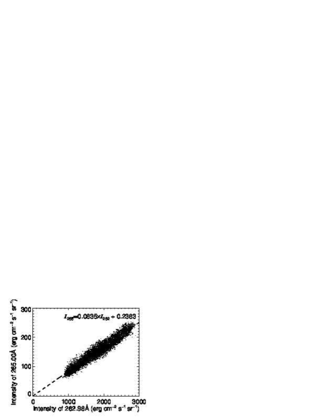
Fig. 5.11: Left: scatter plot for intensities of Fe xvi $262.98$Å and $265.01$Å derived from the scan data used in Chapter 4. A dashed line indicates a fitted linear function whose representation is written in the upper part. Right: the ratio of intensities between those two emission lines. The average value of the ratio is written in the panel.

We investigated the intensity ratio between Fe xvi $262.98$Å and $265.01$Å here. Since the scan used in this chapter did not include a line core of Fe xvi $265.01$Å, we exploited that used in Chapter 4 which includes both emission lines. Left panel in Fig. 5.11 shows the scatter plot for intensities of Fe xvi $262.98$Å ($I_{262}$) and $265.01$Å ($I_{265}$). A dashed line indicates the fitted linear function, whose slope is $0.0835$ (i.e., the intensity ratio). Right panel shows the histogram for the ratio between the two emission lines ($I_{265}/I_{262}$). The average value of $I_{265}/I_{262}$ is $0.0836\,(\pm 6.1\times 10^{-3})$, which is almost the same as the value obtained from the linear fitting in the left panel.

Appendix 5.B Fe xiv 264.78Å intensity and electron density

We can see a clear positive correlation between peak intensity and electron density in the intensity range larger than $I_{\mathrm{Major}}=2.0\times 10^{3}\,\mathrm{erg}\,\mathrm{cm}^{-2}\,\mathrm{s}^{-1}\,\mathrm{sr}^{-1}\,\text{\AA}^{-1}$ (indicated by a vertical dashed line) while the plot is more scattered below that intensity. Not only the photon noise contributes to this large uncertainty, but also unidentified blended emission lines could do. Therefore we analyzed the data points with $I_{\mathrm{Major}}$ larger than the value which the vertical dashed line indicates.

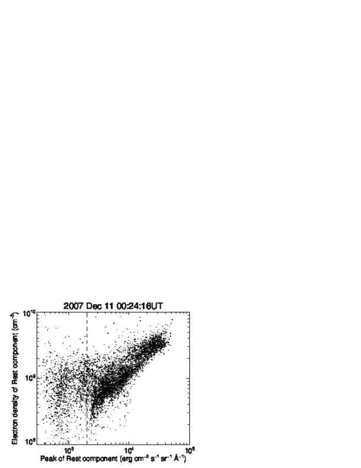
Fig. 5.12: Peak intensity of Fe xiv $264.78$Å vs. electron density deduced from the major component of Fe xiv $264.78$Å and $274.20$Å in the double Gaussian fitting.

Appendix 5.C Electron density at the footpoints of the outflow region

The electron density in NOAA AR10978 was also measured by using a Mg vii emission line pair $280.74$Å/$278.40$Å. This line pair was analyzed since the formation temperature of Mg vii is $\log T\,[\mathrm{K}]=5.8$, which is almost the same as that of Si vii. We can check the validity of the assumption of $n_{\mathrm{Si\textsc{vii}}}=10^{9}\,\mathrm{cm}^{-3}$ in our line profile analysis. The scan used in this chapter did not include these emission lines, so we exploited that used in Chapter 4. The theoretical curve for the intensity ratio of Mg vii $280.74$/$278.40$Å is shown by left panel in Fig. 5.13. This ratio has a good sensitivity to the electron density within the range of $n_{\mathrm{e}}=10^{8\text{--}11}\,\mathrm{cm}^{-3}$ and is suitable for the density diagnostics in the corona as the typical electron density falls within that range.

The spectra were spatially averaged by $5^{\prime\prime}\times 5^{\prime\prime}$ and the intensity of each emission line was calculated by single-Gaussian fitting. Then we derived the electron density at each location referring to the theoretical curve. Right panel in Fig. 5.13 shows the spatial map for the electron density derived from the Mg vii line pair. The color contour was scaled within $n_{\mathrm{e}}=10^{8.4\text{--}9.8}\,\mathrm{cm}^{-3}$. The region painted by black means that the peak intensity of Mg vii $278.40$Å did not exceed $4.0\times 10^{2}\,\mathrm{erg}\,\mathrm{cm}^{-2}\,\mathrm{s}^{-1}\,\mathrm{sr}^{-1}\text{\AA}^{-1}$ below which the spectra were too weak for reliable measurement. White boxes in the map are drawn by taking into account the solar rotation so as to be located at the same position as in Fig. 5.6. The electron density around the eastern and western outflow regions is around $n_{\mathrm{e}}=10^{8.8\text{--}9.2}\,\mathrm{cm}^{-3}$, from which we can conclude that our line profile analysis was valid.

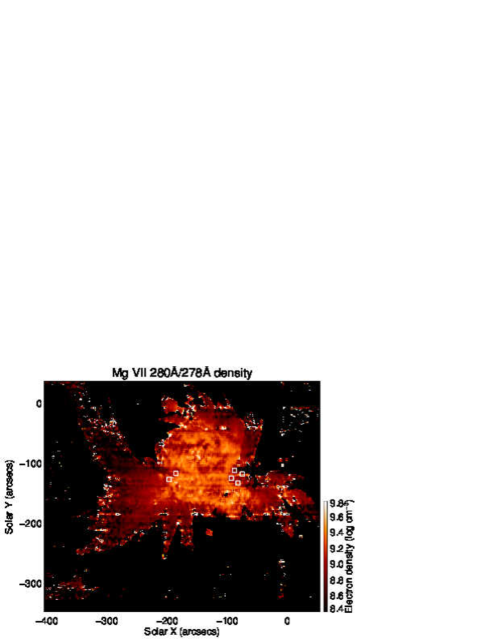
Fig. 5.13: Left: Intensity ratio of Mg vii $280.74$Å/$278.40$Å as a function of electron density. CHIANTI ver. 7 (Dere et al. 1997; Landi et al. 2012) was used in the calculation. Right: electron density map derived by the Mg vii line pair.

Chapter 6 $\lambda$-$n_{\mathrm{e}}$ diagram

We modeled the spectra by the composition of two Gaussians in the above analysis. However, it is difficult to prove whether this assumption is suitable for the outflow regions. There are two alternative approaches to deal such a spectrum consist of more than two Gaussians. One way is to adopt multiple-Gaussian functions (more than two components) and resolve multiple flows existing in a emission line. More number of free parameters we use, the spectra would be fitted with less $\chi^{2}$. But this does not mean that we extracted much more useful physical information from the spectra. The number of local minima increase with complexity of fitting model, and the fitting process becomes an ill-posed problem.

The other way is our new type of plot without assuming any fitting model. Each spectral bin in a pair of a spectrum is used to derive electron density at those each bin, which we refer to as “$\lambda$-$n_{\mathrm{e}}$ diagram” hereafter. In this method, we obtain the measure of electron density of the plasma which have the speed of $v_{\mathrm{Dop}}=c\,(\lambda-\lambda_{0})/\lambda_{0}$ ($\lambda_{0}$: rest wavelength), which is a function of wavelength. Consider a density-sensitive pair of spectra $\phi_{1}(\lambda)$ and $\phi_{2}(\lambda)$ emitted from the same degree of an ion. These emission lines must have the same Doppler velocity because they came from the same degree of the ion, so after converting the variable $\lambda$ into Doppler velocity $v_{\mathrm{Dop}}$ as denoted by $\phi_{i}^{*}(v_{\mathrm{Dop}})=\phi_{i}(\lambda)$ ($i=1,2$), we can calculate the electron density as a function of the Doppler velocity

$$n_{\mathrm{e}}^{*}(v_{\mathrm{Dop}})=R^{-1}\left[\frac{\phi_{2}^{*}(v_{\mathrm{Dop}})}{\phi_{1}^{*}(v_{\mathrm{Dop}})}\right]\,\text{.}$$ (6.1)

The derived $n_{\mathrm{e}}^{*}(v_{\mathrm{Dop}})$ can be converted into a function of wavelength in either spectrum, $n_{\mathrm{e}}(\lambda)$, by the equation of Doppler effect. Function $R(n_{\mathrm{e}})$ is the ratio of intensities from two emission lines which is a function of electron density, so when we know the intensities of two emission lines which are represented as

$$I_{1}=\int\phi_{1}(\lambda)d\lambda\,\text{,}$$ (6.2)

$$I_{2}=\int\phi_{2}(\lambda)d\lambda\,\text{,}$$ (6.3)

electron densities can be usually derived by

$$n_{\mathrm{e}}=R^{-1}\left(\frac{I_{2}}{I_{1}}\right)\,\text{.}$$ (6.4)

As shown in above equations, $\lambda$-$n_{\mathrm{e}}$ diagram represents that of the particles which move with that speed, in other words, we does not obtain the electron density of the whole plasma as an ensemble of Maxwellian distribution. We emphasize the advantage of our method using Eq. (6.1) that even if we do not know the precise functional form of spectra, it gives us the electron density as a function of Doppler velocity without any modeling.

6.1 Method

Making $\lambda$-$n_{\mathrm{e}}$ diagram contains processes: (1) subtraction of blending emission line, (2) adjusting wavelength scale of Fe XIV $264.78$Å to $274.20$Å by interpolation, and (3) density inversion at each spectral pixel. Since the blend of an emission line Si vii $274.18$Å into Fe xiv $274.20$Å was already described in Section 5.3.2, here we explain the processes (2) and (3).

Since the EIS instrument does not have absolute wavelength scale, the corresponding wavelength location of the same velocity in Fe xiv $264.78$Å and $274.20$Å must be determined from data itself as described in Section 5.2.2. Using obtained relation $\lambda_{\mathrm{obs,}274}/\lambda_{\mathrm{obs,}264}=1.0355657$ $(\pm 0.0000044)$, each wavelength value imposed on the spectral window of Fe xiv $264.78$Å was projected onto the values on the spectral window of Fe xiv $274.20$Å by the scaling

$$\tilde{\lambda_{i}}=\alpha\lambda_{264,i}\,\,(\alpha=1.0355657)\,\text{,}$$ (6.5)

where a number $i$ indicates the $i$th spectral pixel in a spectrum of $264.78$Å.

At this point, we projected the spectrum of Fe xiv $264.78$Å into another location in the wavelength direction, which is shifted by as same Doppler shift as the spectrum of Fe xiv $274.20$Å. However, since the spectral pixels on the CCD of EIS are positioned almost linearly as a function of wavelength, the wavelength values of the projected spectrum do not coincide to those of Fe xiv $274.20$Å. In order to align them in a exactly same wavelength values, the projected spectrum of Fe xiv $264.78$Å was interpolated by a cubic spline.

We can calculate the ratio of spectral intensity Fe xiv $264.78$Å/$274.20$Å at each spectral bin. Now we are able to derive the electron density as the same way described in the section 5.3.4. Because intensity at each spectral bin has larger errors compared to the integrated intensity (e.g., double-Gaussian fitting), the estimated errors for the electron density in the $\lambda$-$n_{\mathrm{e}}$ diagram become large especially for the line wing.

6.2 Verification of the method

In order to test the validity of $\lambda$-$n_{\mathrm{e}}$ method, we synthesized spectra of Fe xiv $264.78$Å and $274.20$Å taking into account the spectral resolution of EIS and instrumental broadening. The spectra were composed of two components which represent plasma at the rest and an upflow. While the physical parameters for the major rest component (peak, Doppler velocity, and width) were fixed, those for a minor blueshifted component (i.e., upflow) were taken as variables. We made $\lambda$-$n_{\mathrm{e}}$ diagrams for the minor component with

• electron density of $8.50$, $8.75$, $9.00$, $9.25$, and $9.50$ in the unit of $\log\,\mathrm{cm}^{-3}$,

• intensity of $1$, $5$, $10$, $15$, and $20\,\mathrm{\%}$ (ratio to the major component in Fe xiv $274.20$Å),

• Doppler velocity of $0$, $-50$, $-100$, $-150$, and $-200\,\mathrm{km}\,\mathrm{s}^{-1}$,

• thermal width of $2.0$, $2.5$, $3.0$, $3.5$, and $4.0\,\mathrm{MK}$.

The nonthermal width was not considered in this test because it does not produce any differences essentially. The test for each variable will be given below.

6.2.1 Dependence on electron density

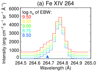
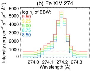
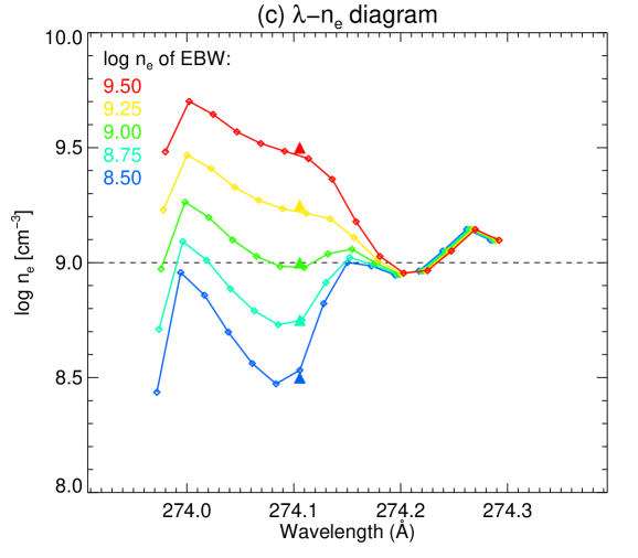
Fig. 6.1: (a) Line profiles of Fe xiv $264.78$Å, (b) Line profiles of Fe xiv $274.20$Å, and (c) $\lambda$-$n_{\mathrm{e}}$ diagrams. Each color indicates different electron density of minor blueshifted component (blue: $8.50$, turquoise: $8.75$, green: $9.00$, yellow: $9.25$, and red: $9.25$ in the unit of $\log\,\mathrm{cm}^{-3}$). Electron density of major component was fixed to $\log n_{\mathrm{e}}\,[\mathrm{cm}^{-3}]=9.00$. The triangles in panel (c) indicate centroid and electron density of the given minor component.

The most important point on $\lambda$-$n_{\mathrm{e}}$ diagram is whether it reflects the electron density of the components which compose spectrum properly or not. In order to test that, we synthesized the spectra which are composed of major component at the rest which has the fixed electron density of $\log n_{\mathrm{e}}[\mathrm{cm}^{-3}]=9.0$ and minor component which has the variable electron density. Five cases ($\log n_{\mathrm{e}}\,[\mathrm{cm}^{-3}]=8.50$, $8.75$, $9.00$, $9.25$, and $9.50$) were analyzed, where the peak ratio of minor/major component was $15\mathrm{\%}$ with fixed upflow speed $v=-100\,\mathrm{km}\,\mathrm{s}^{-1}$. In panel (a) and (b) of Fig. 6.1, the spectra of Fe xiv $264.78$Å and $274.20$Å are respectively shown. Colors (blue, turquoise, yellow, green, and red) indicate the five cases calculated here. After converting the wavelength scale of $264.78$Å to $274.20$Å, $\lambda$-$n_{\mathrm{e}}$ were obtained as shown in panel (c) of Fig. 6.1. The triangles in panel (c) indicate centroid and electron density of the given minor component. It is clear that those $\lambda$-$n_{\mathrm{e}}$ diagrams well reflect the change of the electron density from $\log n_{\mathrm{e}}\,[\mathrm{cm}^{-3}]=8.50\text{--}9.50$. Despite the spectra being composed of only two components, $\lambda$-$n_{\mathrm{e}}$ diagrams do not become a step function but a smooth function. This is natural because the two Gaussians in the spectra contribute each other by their overlapping wings. We claim that the method proposed here ($\lambda$-$n_{\mathrm{e}}$) is a good indicative of the electron density of components in the spectrum.

6.2.2 Dependence on intensity

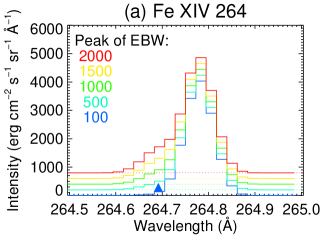
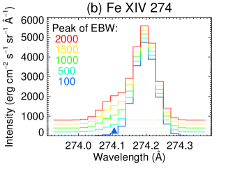
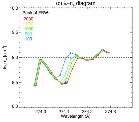
Fig. 6.2: (a) Synthetic line profiles of Fe xiv $264.78$Å, (b) Synthetic line profiles of Fe xiv $274.20$Å, and (c) $\lambda$-$n_{\mathrm{e}}$ diagrams. Each color indicates different intensity of minor blueshifted component (blue: $1$%, turquoise: $5$%, green: $10$%, yellow: $15$%, and red: $20$% of the major rest component). Intensity of the major rest component was fixed.

The dependence of $\lambda$-$n_{\mathrm{e}}$ diagram on the intensity of minor component is relatively trivial compared to previous section. As same as Fig. 6.1, the spectra of Fe xiv $264.78$Å and $274.20$Å, and $\lambda$-$n_{\mathrm{e}}$ diagrams are respectively shown in panel (a), (b), and (c) of Fig. 6.2. Colors indicate the five cases for variable relative intensity calculated here(blue: $1\mathrm{\%}$, turquoise: $5\,\mathrm{\%}$, green: $10\,\mathrm{\%}$, yellow: $15\,\mathrm{\%}$, and red: $20\,\mathrm{\%}$ of the major rest component). The blue triangle in panel (c) indicates centroid and electron density of given minor component. Note that in this test of intensity, those two quantities were fixed ($v=-100\,\mathrm{km}\,\mathrm{s}^{-1}$ and $\log n_{\mathrm{e}}\,[\mathrm{cm}^{-3}]=8.5$). As the intensity of minor blueshifted component increases (i.e., blue to red), dip around $274.07$–$274.10$Å becomes distinct. This is simply because the region between two components is dominated by the major component when the minor component has relatively small peak. On the other hand, the blue side (i.e., shorter wavelength) of the minor component around $274.0$–$274.04$Å does not change significantly for the five cases. Although the location of the dip moves by a change in the relative intensity to a certain extent, the tendency of $\lambda$-$n_{\mathrm{e}}$ diagrams for relative intensity larger than $5\,\mathrm{\%}$ are very similar and well reflect the input electron density, in other words, they are useful for us to know the existence of tenuous upflow.

6.2.3 Dependence on velocity

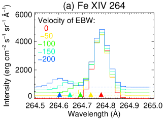
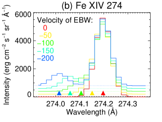
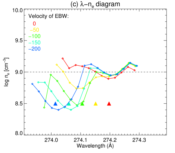
Fig. 6.3: (a) Synthetic line profiles of Fe xiv $264.78$Å, (b) Synthetic line profiles of Fe xiv $274.20$Å, and (c) $\lambda$-$n_{\mathrm{e}}$ diagrams. Each color indicates different velocity of minor blueshifted component (blue: $0\,\mathrm{km}\,\mathrm{s}^{-1}$, turquoise: $-50\,\mathrm{km}\,\mathrm{s}^{-1}$, green: $-100\,\mathrm{km}\,\mathrm{s}^{-1}$, yellow: $-150\,\mathrm{km}\,\mathrm{s}^{-1}$, and red: $-200\,\mathrm{km}\,\mathrm{s}^{-1}$). The major rest component was at rest ($0\,\mathrm{km}\,\mathrm{s}^{-1}$).

The dependence of $\lambda$-$n_{\mathrm{e}}$ diagram on the Doppler velocity of minor component is obvious. The spectra of Fe xiv $264.78$Å and $274.20$Å, and $\lambda$-$n_{\mathrm{e}}$ diagrams are respectively shown in panel (a), (b), and (c) of Fig. 6.3. Colors indicate the five cases for variable Doppler velocity calculated (blue: $0\,\mathrm{km}\,\mathrm{s}^{-1}$, turquoise: $-50\,\mathrm{km}\,\mathrm{s}^{-1}$, green: $-100\,\mathrm{km}\,\mathrm{s}^{-1}$, yellow: $-150\,\mathrm{km}\,\mathrm{s}^{-1}$, and red: $-200\,\mathrm{km}\,\mathrm{s}^{-1}$). Major rest component was at rest ($0\,\mathrm{km}\,\mathrm{s}^{-1}$) with the electron density of $\log n_{\mathrm{e}}\,[\mathrm{cm}^{-3}]=9.0$. The triangles in panel (c) indicate centroid and electron density of given minor component. The relative intensity of minor component is $15\,\mathrm{\%}$ of that of major component and the electron density of minor component was set to $\log n_{\mathrm{e}}\,[\mathrm{cm}^{-3}]=8.5$ in all five cases here. The location of dips in $\lambda$-$n_{\mathrm{e}}$ diagram well represent the centroid position of the input minor component when two components are separated so that the spectrum is dominated by themselves near their centroids. This is not the case for $v=-50\,\mathrm{km}\,\mathrm{s}^{-1}$ (i.e., yellow), where those two components are not separated so well. In this case, $\lambda$-$n_{\mathrm{e}}$ diagram gradually decreases from longer to shorter wavelength. One advantage of the method described here is that we are able to know the tendency of electron density of upflow/downflow without any fitting to the spectrum which might produce spurious result occasionally.

6.2.4 Dependence on thermal width

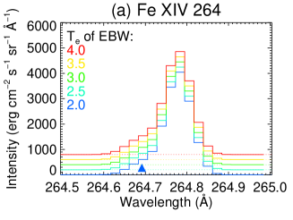
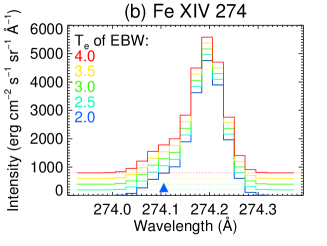
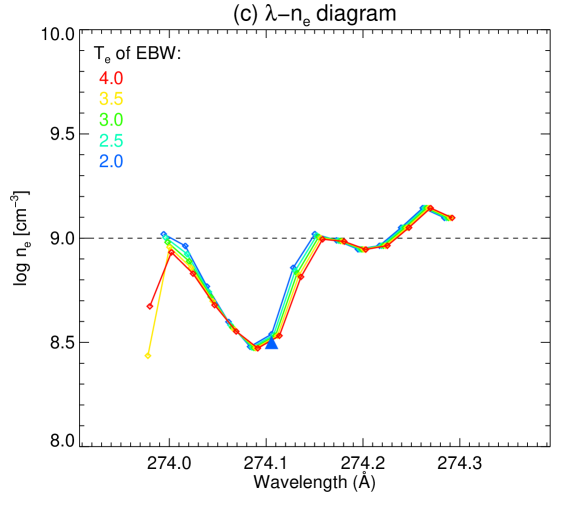
Fig. 6.4: (a) Synthetic line profiles of Fe xiv $264.78$Å, (b) Synthetic line profiles of Fe xiv $274.20$Å, and (c) $\lambda$-$N_{\mathrm{e}}$ diagrams. Each color indicates different thermal width of minor blueshifted component (blue: $2.0\,\mathrm{MK}$, turquoise: $2.5\,\mathrm{MK}$, green: $3.0\,\mathrm{MK}$, yellow: $3.5\,\mathrm{MK}$, and red: $4.0\,\mathrm{MK}$). Thermal width of major component was fixed to $2.0\,\mathrm{MK}$.

The thermal width of minor component can be considered to have less influence on $\lambda$-$n_{\mathrm{e}}$ diagram since the instrumental width of EIS is around $30\,\mathrm{km}\,\mathrm{s}^{-1}$ ($0.027$Å), which corresponds to the thermal width of plasma with temperature of $5\,\mathrm{MK}$. Taking into account the fact that the Differential emission measure analysis revealed that the temperature of the upflow is within $\log T\,[\mathrm{K}]=6.1$–$6.5$ (Brooks & Warren 2011), we test the case for the temperature of minor component from $2$–$4\,\mathrm{MK}$. The spectra of Fe xiv $264.78$Å and $274.20$Å, and $\lambda$-$n_{\mathrm{e}}$ diagrams are respectively shown in panel (a), (b), and (c) of Fig. 6.4. Colors indicate the five cases for variable thermal width calculated (blue: $2.0\,\mathrm{MK}$, turquoise: $2.5\,\mathrm{MK}$, green: $3.0\,\mathrm{MK}$, yellow: $3.5\,\mathrm{MK}$, and red: $4.0\,\mathrm{MK}$). The blue triangle in panel (c) indicates centroid and electron density of given minor component. As we expected, $\lambda$-$n_{\mathrm{e}}$ diagrams show much less change with increasing thermal width compared to the previous three sections.

The tests above for the four variables (i.e., density, intensity, velocity, and thermal width) indicate that the method proposed here ($\lambda$-$n_{\mathrm{e}}$ diagram) is a powerful diagnostic tool for coronal plasma which may constitute from several component along the line of sight and form non-single-Gaussian line profile. In the next section, we exploit this $\lambda$-$n_{\mathrm{e}}$ diagram so that the result obtained by double-Gaussian fitting would (i.e., upflows are more tenuous than the rest component) be confirmed.

6.2.5 Binning effect

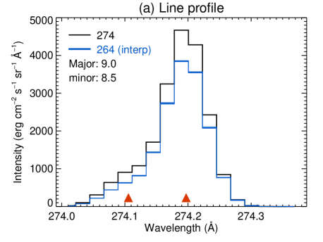
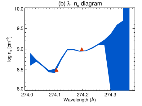
Fig. 6.5: (a) Synthetic line profiles of $274.20$Å (black) and $264.78$Å (blue) with adjusted wavelength. Red triangles indicate the centroid of the two Gaussians given. The electron density of major and minor component is respectively $10^{8.5}$ and $10^{9}\,\mathrm{cm}^{-3}$. The Blue line profile has a finite width in the vertical axis (though it is narrow), which shows the range when changing the binning position at $264.78$Å spectral window. (b) $\lambda$-$n_{\mathrm{e}}$ diagram with varying binning position at $264.78$Å spectral window. The vertical width of the diagram shows the range. Red triangles show the same meaning as in panel (a).

As an instrumental effect, the binning of the wavelength direction may contribute to the uncertainty in $\lambda$-$n_{\mathrm{e}}$ diagram. In order to test this possibility, we moved the position of binning at Fe xiv $264.78$Å spectral window consecutively by $0.001$Å up to $0.05$Å (cf. spectral pixel of EIS $\simeq 0.0223$Å). The results are shown in Fig. 6.5. Panel (a) shows synthetic line profiles of Fe xiv $274.20$Å (black profile) and tested $264.78$Å (blue profile). Red triangles indicate the centroid of the two Gaussians given. The electron density of major and minor component is respectively $10^{8.5}$ and $10^{9}\,\mathrm{cm}^{-3}$. The Blue line profile has a finite width in the vertical axis (though it is narrow and hard to see), which shows the range when changing the binning position at $264.78$Å spectral window. Panel (b) shows $\lambda$-$n_{\mathrm{e}}$ diagram with varying binning position at $264.78$Å spectral window. The vertical width of the diagram shows the range of values which derived $\lambda$-$n_{\mathrm{e}}$ diagrams took. Red triangles show the same meaning as in panel (a). From panel (b), it can be seen that the uncertainty caused by the position of binning does not exceed $0.1\,\log\,\mathrm{cm}^{-3}$ at the location where we are interested in, but becomes quite larger away from the emission line center because of the low intensity.

6.3 $\lambda$-$n_{\mathrm{e}}$ diagram in AR10978

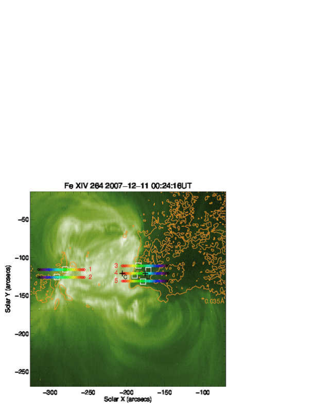
Fig. 6.6: Intensity map of Fe xiv $264.78$Å obtained with EIS. Five arrays of colored diamonds (red–violet) are the locations where $\lambda$-$n_{\mathrm{e}}$ diagrams were made. The locations cut across the active region core and the outflow region. Orange contour indicates the line width of $0.035$Å.

The electron density of the outflow region in AR 10978 is investigated through $\lambda$-$n_{\mathrm{e}}$ diagram here. Fig. 6.6 shows intensity map of Fe xiv $264.78$Å obtained with EIS. Orange contours indicate the line width of $0.035$Å, which becomes an indication of the outflows. Five horizontal arrays of colored diamonds (red–violet) which cut across the active region core and the outflow region are the locations where we made $\lambda$-$n_{\mathrm{e}}$ diagrams. First, we look at the location indicated by black plus signs named C (core) and U (outflow).

In Fig. 6.7, the line profiles of Fe xiv $274.20$Å, interpolated $264.78$Å and estimated Si vii $274.18$Å (see Section 5.3.2) are respectively shown by solid, dashed, and dotted spectrum in panel (a) for the active region core and (b) for the outflow region. We can see an enhanced blue wing in line profiles of Fe xiv in the outflow region. The vertical dashed lines indicate rough reference of the rest wavelength position $\lambda=274.195$Å which was the average line centroid above the limb in the 2007 December 18 data (possible error up to $0.01$Å).

Panels (c) and (d) in Fig. 6.7 respectively show the $\lambda$-$n_{\mathrm{e}}$ diagram for the active region core and the western outflow region. The horizontal green dotted line in each plot indicate the electron density averaged in the neighbor three spectral bins which are nearest to $\lambda=274.20$Å (i.e., rest wavelength). Those $\lambda$-$n_{\mathrm{e}}$ diagrams in the two locations exhibit a different behavior at shorter wavelength side around $\lambda=274.00\text{--}274.20$Å: the diagram in the active region core is roughly constant while that in the western outflow region slightly decreases at the shorter wavelength. The number written in the upper left corner of each plot indicates the linear slope fitted within the wavelength range $\lambda\leq 274.20$Å. This implies that the electron density of the outflows (i.e., shorter wavelength side) is smaller than that of the major rest component.

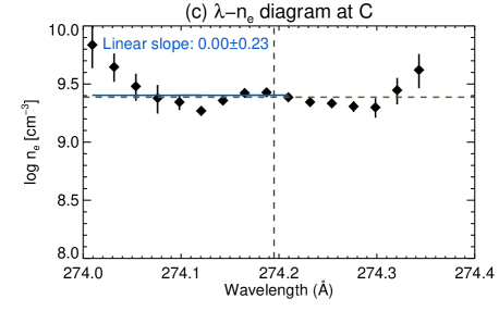
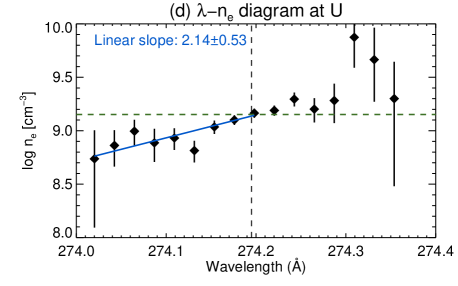
Fig. 6.7: (a) Line profiles of Fe xiv $274.20$Å (solid)/$264.78$Å (dashed; adjusted to the wavelength scale of $274.20$Å) and Si vii $274.18$Å (dotted) estimated from $275.35$Å at the active region core. (b) Line profiles at the outflow region. (c) $\lambda$-$n_{\mathrm{e}}$ diagram at the active region core. (d) $\lambda$-$n_{\mathrm{e}}$ diagram at the outflow region.

In order to confirm the above implication more robust, we see the variation of $\lambda$-$n_{\mathrm{e}}$ diagram along $x$ direction from the active region core to the outflow regions. The selected region spans from the active region core (red diamond) to the outflow region (violet diamond) as seen in Fig. 6.6. The boundary of the active region core corresponds to the color between yellow and light green. The $\lambda$-$n_{\mathrm{e}}$ diagrams at each cut (1–5) are plotted in Fig. 6.8. We can see clear change of the $\lambda$-$n_{\mathrm{e}}$ diagrams with colors. The $\lambda$-$n_{\mathrm{e}}$ diagrams for cut 1 show a small hump around $274.00$–$274.10$Å representing that EBW component has larger electron density than the major component, though the hump at almost all locations (red–black) might mean that it was caused by an anomalous pixel (e.g., warm pixel). Both for cut 1 and 2, the diagrams show flat or slightly decreasing behavior as a function of wavelength at all locations. These behaviors are consistent with the result obtained in Chapter 5 (region U1 and U2) which indicated that the electron density of the outflows in the eastern edge is almost the same or slightly larger. On the other hand, in the western outflow region (cut 3–5), those for the outflow region show a dip around $274.10$Å. This wavelength corresponds to $v=-110\,\mathrm{km}\,\mathrm{s}^{-1}$ for the emission line Fe xiv $274.20$Å, from which it is implied that the outflows in the western edge are composed of less dense plasma compared to the rest plasma (i.e., around $274.20$Å) existing along the line of sight. Note that this velocity does not mean that of the upflows because no fitting was applied in $\lambda$-$n_{\mathrm{e}}$ diagram.

The electron density of EBW component evaluated from $\lambda$-$n_{\mathrm{e}}$ diagrams around $\lambda=274.10$Å was $\log n_{\mathrm{e}}\,[\mathrm{cm}^{-3}]=9.0\text{--}9.2$ in the eastern outflow region, and $\log n_{\mathrm{e}}\,[\mathrm{cm}^{-3}]=8.5\text{--}9.0$ in the western outflow region, which also coincides the result obtained in the previous chapter. By exploiting $\lambda$-$n_{\mathrm{e}}$ diagram as a new diagnostic tool, we now support the result obtained by double-Gaussian fitting in Chapter 5.

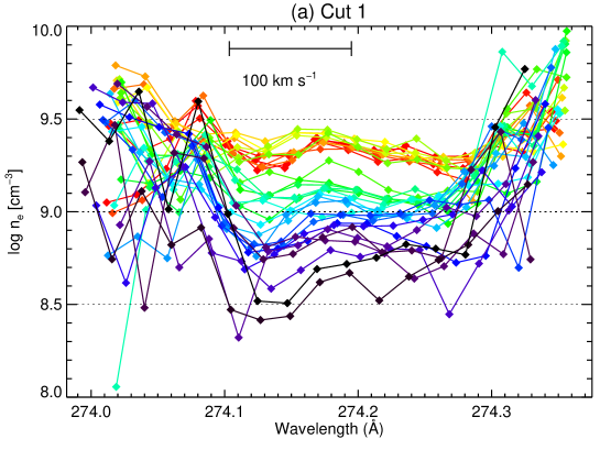
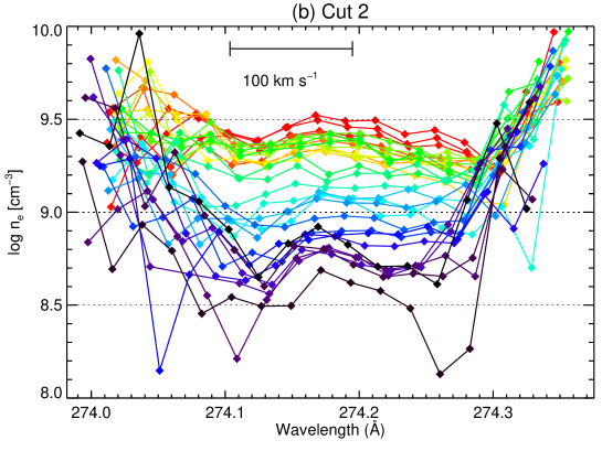
Fig. 6.8: $\lambda$-$n_{\mathrm{e}}$ diagrams at the locations indicated by colored diamonds in Fig. 6.6 (Cut 1 and 2; including the eastern outflow region).

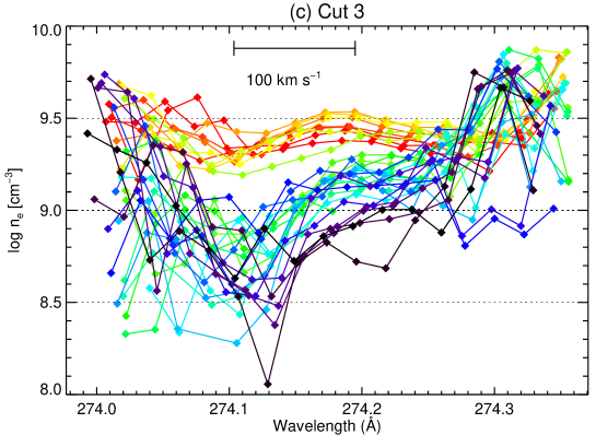
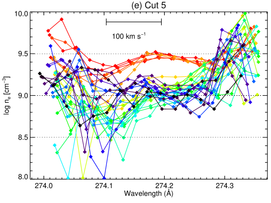
Fig. 6.8: Continued. $\lambda$-$n_{\mathrm{e}}$ diagrams at the locations indicated by colored diamonds in Fig. 6.6 (Cut 3–5; including the western outflow region).

6.4 Summary and discussion

We introduced a density diagnostics from a new point of view in this chapter. Electron density derived in our method is a function of Doppler velocity or wavelength (Eq. 6.1), referred to as $\lambda$-$n_{\mathrm{e}}$ diagram, which was found to be a good indication of the electron density of minor components in a line profile. The method has an advantage that it does not depend any fitting model which might be ill-posed in some cases. Our aim was to evaluate the electron density of the outflow seen at the edge of the active region, and reinforce the result obtained in Chapter 5.

Using a density-sensitive emission line pair Fe xiv $264.78$Å/$274.20$Å, we studied $n_{\mathrm{e}}(\lambda)$ by making $\lambda$-$n_{\mathrm{e}}$ diagrams at the active region core and the outflow regions. The increase in the diagrams was seen on the longer wavelength side for both structures, but we could not find whether that behavior actually implies the physical situation at present. The diagrams for the active region core were flat around $\log n_{\mathrm{e}}\,[\mathrm{cm}]^{-3}\simeq 9.5$, while those for the outflow regions exhibit some characteristic behaviors at shorter wavelength side. They show a small hump around $v=-110\,\mathrm{km}\,\mathrm{s}^{-1}$ in the eastern region (cut 1 and 2 in Fig. 6.6), and a decrease trend from $\log n_{\mathrm{e}}\,[\mathrm{cm}^{-3}]=9.0$ to $\log n_{\mathrm{e}}\,[\mathrm{cm}^{-3}]=8.5$ in a velocity scale of $100\,\mathrm{km}\,\mathrm{s}^{-1}$ in the western outflow region (cut 3–5 in Fig. 6.6) as seen in Fig. 6.8. Thus we confirmed the results obtained in Chapter 5 through our new method independent of the double-Gaussian fitting.

Chapter 7 Summary and discussion

7.1 Summary of the results

Here we summarize the results obtained in Chapter 3–6.

Average Doppler shifts of the quiet region (Chapter 3)

Two meridional scans were analyzed, from which we determined the Doppler velocity of the quiet region within $\log T\,[\mathrm{K}]=5.7$–$6.3$ in the accuracy of $\simeq 3\,\mathrm{km}\,\mathrm{s}^{-1}$ for the first time. It was shown that emission lines below $\log T\,[\mathrm{K}]=6.0$ have Doppler velocity of almost zero with an error of $1$–$3\,\mathrm{km}\,\mathrm{s}^{-1}$, while those above that temperature are blueshifted with gradually increasing magnitude: $v=-6.3\pm 2.1\,\mathrm{km}\,\mathrm{s}^{-1}$ at $\log T\,[\mathrm{K}]=6.25$ (Fe xiii). These Doppler velocities were used as a reference in Chapter 4.

Doppler velocity measurement for AR outflows (Chapter 4)

Doppler velocities for emission lines with the formation temperature of $\log T\,[\mathrm{K}]=5.5$–$6.5$ were measured by the single-Gaussian fitting in the active region NOAA AR10978. The outflow regions and fan loops were distinguished in terms of the Doppler velocity in the transiton region temperature.

• The line profiles with the formation temperature of $\log T\,[\mathrm{K}]=6.1$–$6.3$ have significant EBW corresponding to $v\sim-100\,\mathrm{km}\,\mathrm{s}^{-1}$ in the outflow regions, while those below $\log T\,[\mathrm{K}]=6.0$ and above $\log T\,[\mathrm{K}]=6.4$ did not.

• The Doppler velocities within $\log T\,[\mathrm{K}]=5.7$–$6.3$ were all blueshifted by $v=-20\,\mathrm{km}\,\mathrm{s}^{-1}$ (i.e., upflow) in the outflow regions. The clear blueshift of the transition region lines were confirmed for the first time precisely in the outflow regions.

• Fan loops adjacent to the outflow regions exhibited decreasing Doppler velocity from $v=20\,\mathrm{km}\,\mathrm{s}^{-1}$ at the transition region temperature to $-10\,\mathrm{km}\,\mathrm{s}^{-1}$ at the coronal temperature, consistent with previous observations.

Density of the upflows (Chapter 5)

The electron density of the outflows was derived by using a density-sensitive line pair Fe xiv $264.78$Å/$274.20$Å. The double-Gaussian fitting was simultaneously applied to the two emission line profiles from the physical requirement. Obtained Doppler velocities, electron densities, and column depths are listed in Table 7.1 (excerpt from Table 5.1).

• We found that the magnitude relationship between the electron density of the major component and that of EBW component is opposite in the eastern and western outflow regions.

• The column depths calculated from the obtained electron density indicate that the volume amount of the upflows is much less than that of the major component in the eastern outflow region, while the former dominates the latter in the western outflow region.

Table 7.1: Derived physical quantities in the eastern and western outflow regions. Topology indicates the magnetic connectivity which was inferred from the coronal magnetic field (constructed in Appendix A) and the appearance of Doppler velocity maps: open means that a structure extends far from its footpoint (i.e., very long), and close means that a structure forms a corona loop.

	$v_{\mathrm{Dop}}\,(\mathrm{km}\,\mathrm{s}^{-1})$		$\log n_{\mathrm{e}}\,[\mathrm{cm}^{-3}]$		$\log h\,[\mathrm{cm}]$		Topology
	EBW	Major	EBW	Major	EBW	Major
Eastern	$-88.8\pm 15.2$	$-4.2\pm 1.4$	$9.06\pm 0.14$	$9.01\pm 0.11$	$7.36\pm 0.43$	$8.51\pm 0.16$	closed
Western	$-62.0\pm 16.0$	$0.1\pm 2.7$	$8.60\pm 0.22$	$9.22\pm 0.14$	$8.53\pm 0.41$	$7.74\pm 0.15$	open

$\lambda$-$n_{\mathrm{e}}$ diagram (Chapter 6)

We developed a new method in line profile analysis to investigate the electron density of EBW component from another point of view. The advantage of the method is that it does not depend on fitting models, from which we reinforced the results obtained in Chapter 5.

7.2 Temperature of the outflows

The line profiles in the outflow regions are characterized by their EBW with a speed up to $100\,\mathrm{km}\,\mathrm{s}^{-1}$ within the formation temperature of $\log T\,[\mathrm{K}]=6.1$–$6.3$. This implies that the outflows are mainly composed of the plasma in that temperature range. The differential emission measure (DEM) analysis of the outflows indicated that there is a peak at $1.4$–$1.8\,\mathrm{MK}$ (i.e., around $\log T\,[\mathrm{K}]=6.2$), which is consistent with our result. Though it has not been focused on in the literature, we found that the line profiles with the formation temperature of $\log T\,[\mathrm{K}]\geq 6.4$ (i.e., Fe xvi and S xiii) did not show the signature of EBW in the outflow region. This means that the hot plasma does not exist in the outflows, which leads to the implication that the corona in the outflow regions are heated up to at most $\log T\,[\mathrm{K}]\leq 6.3$. Note that the lack of EBW in those hot coronal lines might indicate the scattered spectra from the active region core, since Fe xvi and S xiii are much brighter at the core as already discussed in section 4.6.

It was shown that the transition region lines (e.g., Si vii and Mg vii; $\log T\,[\mathrm{K}]=5.8$) are symmetric in the outflow regions and did not have EBW, but they are significantly blueshifted by around $v=-20\,\mathrm{km}\,\mathrm{s}^{-1}$. It can be straightforwardly interpreted as the plasma with a temperature around $\log T\,[\mathrm{K}]=5.8$ were all flowing upward with a speed of $v=-20\,\mathrm{km}\,\mathrm{s}^{-1}$. But since the line width was broadened as seen in Fig. 4.5, we suppose two another possibilities: (1) the upflows in the transition region lines are actually hotter than their formation temperature, or (2) the line profiles from the transition region represent a superposition of several components which have different line-of-sight velocities. The interpretation of the line broadening in terms of the high temperature leads to the temperature of $T\simeq 1.5\,\mathrm{MK}$ (i.e., $\log T\,[\mathrm{K}]=6.2$) as calculated from the line width of $W\simeq 0.045$Å in the outflow regions and $W\simeq 0.030$Å in fan loops. However, since the emission lines around $\log T\,[\mathrm{K}]=6.2$ (i.e., Fe xi–xiii) clearly exhibit the existence of EBW, the line profiles at $\log T\,[\mathrm{K}]=5.8$ must have EBW if the first possibility is the case. However, the transition region lines showed symmetric, therefore the first possibility should be excluded. On the other hand, the second possibility remains reasonable when the emission measure of components in the line profiles is similar to each other. In that case, the line profiles have a broadened and rather symmetric shape. We do not know at present whether the components in the line profiles are all blueshifted or some of them are redshifted, which may become important to consider what is occurring at the transition region. One idea to test both possibilities is that we compare the line profiles both at the disk center and near at the limb. The line profiles will keep their line width when the first possibility is the case, while they will become less broadened near at the limb than at the disk center when the second possibility is the case. The fact that the upflow speed in the transition region lines is much slower than that in the coronal lines may indicate the acceleration of the outflows from the transition region to the corona.

7.3 Outflow region and fan loops

Emission lines with the formation temperature $\log T\,[\mathrm{K}]\leq 6.4$ were all blueshifted by $v\leq-20\,\mathrm{km}\,\mathrm{s}^{-1}$ (i.e., upflow) in the outflow region as shown in Chapter 4 (Fig. 4.15). This result is not consistent with Warren et al. (2011), one of few previous studies on the temperature dependence of outflow regions, which reported redshift of the transition region lines and blueshift of coronal lines. This contradiction originates in the fact that they actually referred to the property of fan loops (Fig. 3 and 4 in their paper). The outflows and fan loops are often located in neighboring region which leads to the confusing statement in the literature. We found a clear difference in the temperature dependence of the Doppler velocity between the outflow region and surrounding fan loops. Baker et al. (2009) previously showed that an emission line from Si vii ($\log T\,[\mathrm{K}]=5.8$) exhibits blueshift by several $\mathrm{km}\,\mathrm{s}^{-1}$. However, their measurement included the uncertainty of $\sim 10\,\mathrm{km}\,\mathrm{s}^{-1}$. We have confirmed the blueshifts of emission lines with the formation temperature below $\log T\,[\mathrm{K}]=6.0$ for the first time with much more careful procedures in determining the Doppler velocities (i.e., accuracy better than $5\,\mathrm{km}\,\mathrm{s}^{-1}$; see Chapter 3).

Table 7.2: Estimated energy loss from the outflow regions and fan loops. The factor $q$ in the radiative flux $Q$ represents the radiative loss per volume noted in the main text. We use the thermal diffusion coefficient of $\kappa_{0}=10^{-6}\,\mathrm{erg}\,\mathrm{cm}^{-1}\,\mathrm{s}^{-1}\,\mathrm{K}^{-7/2}$.

				Energy flux ($\mathrm{erg}\,\mathrm{cm}^{-2}\,\mathrm{s}^{-1}$)
	Length	$T$	Speed	Radiation	Conduction	Kinetic energy	Total
	($\mathrm{Mm}$)	($\mathrm{MK}$)	($\mathrm{km}\,\mathrm{s}^{-1}$)	$Q=qL$	$F_{\mathrm{c}}\approx\kappa_{0}\left|T\right|^{7/2}L^{-1}$	$K=\left[(1/2)\rho v^{2}\right]v$
Outflows	$\geq 100$	$1$–$2$	$100$	$(1\text{--}10)\times 10^{5}$	$(1\text{--}11)\times 10^{5}$	$(2\text{--}5)\times 10^{5}$	$(4\text{--}20)\times 10^{5}$
Fan loops	$100$–$200$	$0.8$	$20$	$(1\text{--}13)\times 10^{5}$	$(3\text{--}5)\times 10^{4}$	$4\times 10^{3}$	$(1\text{--}13)\times 10^{5}$

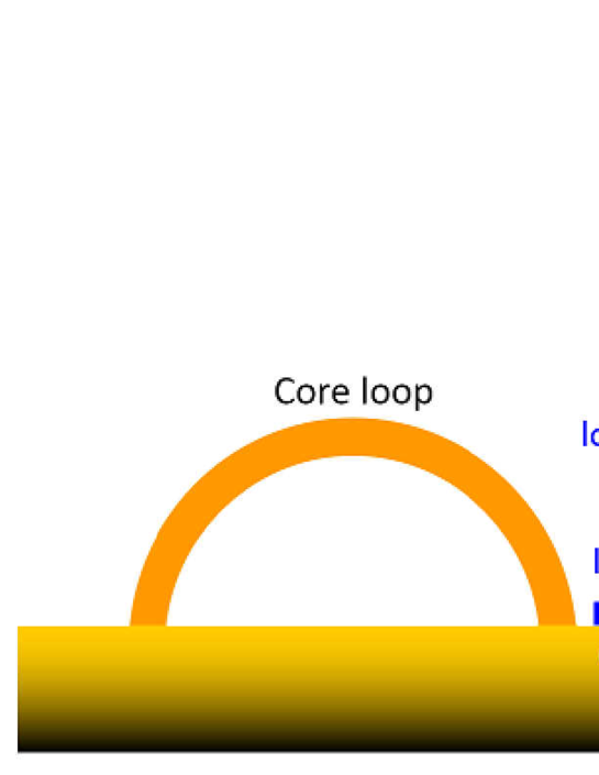
Fig. 7.1: Schematic view of the outflow and a fan loop.

The fan loops extended from distinct footpoints beside the outflow region, while blueshifted region in Fe xii–xiii Doppler maps (see Section 4.4.1) was elongated from the outflow region. No any distinct loops were seen in the outflow region observed with TRACE $171$Å passband (see Section A.3). Since EUV emission from the corona is optically thin, it is not obvious whether the temperature dependence of the Doppler velocity (i.e., $v\geq 0$ for the transition region lines and $v\leq 0$ for the coronal lines) represents the characteristics of fan loops. We mention a possibility that our line of sight penetrates the fan loops and an elongated structure from the outflow region as shown in Fig. 7.1, which suggests that (1) the temperature dependence of fan loops would be a line-of-sight superposition of two structures, and (2) EBW component has been considered to be an indication of upwardly propagating disturbances in fan loops (McIntosh et al. 2012), but it may be originated from the outflow region.

In order to consider the energetics of the outflow region and fan loops, we estimated the radiative flux ($Q$), thermal conductive flux ($F_{\mathrm{c}}$), and the kinetic energy flux ($K$) in both structures as listed in Table 7.2. The temperatures for both structures are taken by the fact that the deviation from single Gaussian has a peak around $\log T\,[\mathrm{K}]=6.2$ (i.e., a large EBW component relative to the major component) for the outflows, and fan loops are most clearly seen in Fe viii and Si vii. We used the radiative loss function $q=n_{\mathrm{e}}^{2}\times 10^{-22}\,\mathrm{erg}\,\mathrm{cm}^{3}\,\mathrm{s}^{-1}$ ($\log T\,[\mathrm{K}]=5.75$–$6.3$; Rosner et al. 1978). The relation of magnitude becomes $Q\approx F_{\mathrm{c}}\approx K$ for the outflow region, and $Q\gg F_{\mathrm{c}}>K$ for fan loops. The total fluxes, a measure of the coronal heating term, were comparable for the outflow region and fan loops. These relations may indicate that a significant part of the heating is converted into the kinetic energy (i.e., the outflow), while the radiation becomes the dominant loss and the thermal conduction plays less important role in fan loops. The reason why they distribute the energy in different ways even with the same magnitude of the energy input could be important to better understand the formation process of those coronal structures, which should be investigated in the future. The observation which tracks the temporal variability both the outflow region and fan loops enables us to study the relationship between neighboring those structures and could shed the light to such a problem.

7.4 Steady flow along coronal loops

Taking the western outflow region as an example case, we consider the possibility whether the outflow can be the siphon flow, which is unidirectional flow along a coronal loop induced by the gas pressure difference between two footpoints of the coronal loop (Cargill & Priest 1980). Here we check the conservation of mass flux and the difference of the gas pressure at both footpoints determined by the field lines constructed from an MDI magnetogram (see Appendix). The conservation of mass flux can be represented as $n_{\mathrm{e}}\,\lvert v\rvert\,A=\mathrm{const.}$, where $A$ is a cross section of the magnetic flux tube ($\propto\lvert B\rvert^{-1}$). The equation can be modified as $n_{\mathrm{e}}\,\lvert v_{\mathrm{Dop}}\rvert/\lvert B_{z}\rvert=\mathrm{const.}$.

Fig. 7.2: Electron density map derived by Mg vii $280.74$Å/$278.40$Å line ratio. Four blue lines are the field lines rooted at the western outflow region which were extrapolated from the magnetogram (see Appendix A). Their footpoints are indicated by circles.

Fig. 7.2 shows the electron density map derived by using a Mg line pair $280.74$Å/$278.40$Å described in Section 5.C. Four blue lines indicate projected field lines. The electron density and Doppler velocity of Mg vii in the western outflow region were respectively $n_{\mathrm{e}}=10^{8.7\text{--}8.9}\,\mathrm{cm}^{-3}$ and $v_{\mathrm{Dop}}=-29.3\,\text{--}\,{-15.8}\,\mathrm{km}\,\mathrm{s}^{-1}$, while those at the opposite side was $n_{\mathrm{e}}=10^{9.3\text{--}9.4}\,\mathrm{cm}^{-3}$ and $v_{\mathrm{Dop}}=-0.21\,\text{--}\,10.4\,\mathrm{km}\,\mathrm{s}^{-1}$. The magnetic field strength in the outflow region was $B_{z}=-191\,\text{--}\,{-305}\,\mathrm{G}$ while that at the opposite side was $B_{z}=285\text{--}810\,\mathrm{G}$. The ratio of the mass flux of the opposite side to the outflow region becomes $3.3\times 10^{-1}$, $1.3$, $2.8\times 10^{-2}$, $2.7\times 10^{-1}$ for the four field lines. Since the mass flux at both footpoints does not balance (i.e., too much supply for three out of four field lines checked), the steady flow along the coronal loops would not be realized. Note that since the magnetic field strengths were measured at the photosphere while the Doppler velocities and electron densities were measured in the transition region, the above mass flux calculation may be a rough estimate.

We also evaluate the pressure at the footpoints of loops connecting the western outflow region and the opposite side. If we assume that the plasma emitting the emission line has the same temperature at both footpoints, the gas pressure in the western outflow region becomes $p_{\mathrm{gas}}=(4.4\text{--}6.9)\times 10^{-2}\,\mathrm{dyne}\,\mathrm{cm}^{-2}$, and that at the opposite side becomes $(1.7\text{--}2.2)\times 10^{-1}\,\mathrm{dyne}\,\mathrm{cm}^{-2}$. The gas pressure at the western outflow region is smaller than that at the opposite side by an order of magnitude, which indicates that the outflow cannot be the siphon flow along the coronal loops. This implies that the magnetic field extrapolation by potential calculation is not correct, or the field lines may continuously expand into higher location which can produce steady upflow from the footpoints.

Some of previous observations interpreted the outflows as the source region of the slow solar wind (Sakao et al. 2007; Harra et al. 2008; Baker et al. 2009). Our results indicate that not only coronal lines but also the transition region lines are blueshifted, and clear EBW (i.e., fast component) exists only in the coronal line profiles, both of which are compatible with the Parker’s solution for the solar wind (Parker 1958) since it predicts strong acceleration near the bottom of the corona and monotonically increasing velocity into the interplanetary space. However, the location where EBW becomes prominent (i.e., line broadening, Hara et al. 2008) is highly localized at the edges of the active region, and there is no EBW in the extended structure from the outflow regions. It means that such fast component may be decelerated along the magnetic structure, which is not consistent with the solar wind solution. We suggest two possibilities as follows. (1) The deceleration occurs only due to the line of sight effect. The angle between the line of sight and the magnetic field line is probably larger at the higher altitude. (2) There exists some mechanism such as heating or a change in the magnetic topology, which induces the upflows from the transition region. The direct measurement of the coronal magnetic field in the future will be helpful to test these possibilities.

7.5 Interpretation in terms of impulsive heating

7.5.1 Temperature dependence of the Doppler velocity

When the impulsive heating occurs in a coronal loop, the energy will be transported dominantly through thermal conduction, which abruptly heat the transition region. The transition region loses its energy increase by the radiation, but if the loss is not sufficient to consume the energy increase, the plasma starts to expand into the upper atmosphere. One-dimensional hydrodynamic simulation on the impulsive heating showed that such upflow can be detected by hot emission lines and it has a speed of $\sim 100\,\mathrm{km}\,\mathrm{s}^{-1}$ (Patsourakos & Klimchuk 2006), which is a consistent value to the speed of the upflow component in line profiles of Fe xii–xiv. Several observations linked the outflows to he upflow following an impulsive heating at the outflow regions (Del Zanna 2008; Peter 2010).

There is a major discrepancy in the behavior of the transition region lines between our result and simulation by Patsourakos & Klimchuk (2006). In their simulation, a line profile of Ne viii ($\log T\,[\mathrm{K}]=5.8$) was redshifted by $v\simeq 10\,\mathrm{km}\,\mathrm{s}^{-1}$, which was explained by the plasma draining during the cooling phase. Contrary to the simulation, our analysis indicated that even the transition region lines ($\log T\,[\mathrm{K}]=5.5\text{--}6.0$) are indeed blueshifted by $v\simeq-20\,\mathrm{km}\,\mathrm{s}^{-1}$ as shown in Chapter 4. Thus, we cannot apply the impulsive heating with long time intervals (i.e., leading to the plasma draining) directly to the outflow region.

7.5.2 Analytical estimation of electron density

De Pontieu et al. (2011) proposed that the tip of the spicule is heated up to the coronal temperature (though the heating mechanism has not been revealed), and is injected to the higher atmosphere where the heated plasma form the corona. The electron density of upflows from the tips of the spicules is estimated by Eq. (10) in Klimchuk (2012) which considers the mass conservation,

$$n_{\mathrm{UP,}\,s}\delta h_{s}=n_{c}h_{c}A,$$ (7.1)

where $n_{\mathrm{UP,}\,s}$ is the electron density of an upflow (a suffix $s$ denotes spicule), $\delta$ is the fraction of the spicule that is heated to coronal temperatures, $h_{s}$ is the height of the spicule, $n_{c}$ is the coronal density after the tip of the spicule expands into the corona, $h_{c}$ is the length of coronal loops, and $A$ is the expansion factor of the cross section of coronal loops from the chromosphere to the corona. Using typical coronal values: $n_{c}\simeq 10^{9}\,\mathrm{cm}^{-3}$, $h_{c}\simeq 5\times 10^{9}\,\mathrm{cm}$, $\delta\simeq 10\,\mathrm{\%}$ (De Pontieu et al. 2011), $h_{s}\simeq 10^{9}\,\mathrm{cm}$ in the maximum height, and $A\sim 10$ (this factor has not been determined precisely yet, but is larger than unity), the electron density of upflows is estimated as

$$n_{\mathrm{UP,}\,s}\simeq 5\times 10^{11}\left(\frac{n_{c}}{10^{9}\,\mathrm{cm}^{-3}}\right)\left(\frac{h_{c}}{5\times 10^{9}\,\mathrm{cm}}\right)\left(\frac{A}{10}\right)\left(\frac{\delta}{0.1}\right)^{-1}\left(\frac{h_{s}}{10^{9}\,\mathrm{cm}}\right)^{-1}\,\mathrm{cm}^{-3}\,\text{.}$$ (7.2)

For impulsive heating, giving the typical energy content of nanoflare (i.e., $10^{24}\,\mathrm{erg}$) and considering the enthalpy flux as a response of the transition region below the corona leads to

$$\frac{5}{2}pv_{\mathrm{UP,}\,\mathrm{i}}=\frac{E_{\mathrm{i}}}{\pi r^{2}_{\mathrm{st}}\tau_{\mathrm{i}}}\,\text{,}$$ (7.3)

where $p$ is the gas pressure of the upflow, $v_{\mathrm{UP,}\,\mathrm{i}}$ is the speed of the upflow, $E_{\mathrm{i}}$ is the released energy by the impulsive heating, $r^{2}_{\mathrm{st}}$ is the radius of the coronal strand (i.e., thin coronal loop as an elemental structure), and $\tau_{\mathrm{i}}$ is the duration of the impulsive heating. Kinetic energy flux can be neglected because the upflow speed is around a half of the sound speed ($\simeq 200\,\mathrm{km}\,\mathrm{s}^{-1}$ at $\log T\,[\mathrm{K}]=6.3$), which means the ratio of the kinetic energy flux to the enthalpy flux is the order of $0.1$. Typical parameters $E_{\mathrm{i}}\sim 10^{24}\,\mathrm{erg}$, $v_{\mathrm{UP,i}}\simeq 100\,\mathrm{km}\,\mathrm{s}^{-1}$, $r^{2}_{\mathrm{st}}\sim 100\,\mathrm{km}$ (moderate estimation considering the coronal filling factor of $0.01$–$0.1$), and $\tau_{\mathrm{i}}\sim 10\text{--}100\,\mathrm{s}$ (this value contains a large uncertainty because of the lack of our knowledge in the present) imply

$$n_{\mathrm{UP,}\,\mathrm{i}}\simeq 5\times 10^{10}\left(\frac{E_{\mathrm{i}}}{10^{24}\,\mathrm{erg}}\right)\left(\frac{r_{\mathrm{st}}}{10^{7}\,\mathrm{cm}}\right)^{-2}\left(\frac{\tau_{\mathrm{i}}}{10\,\mathrm{s}}\right)^{-1}\left(\frac{T_{\mathrm{i}}}{10^{6}\,\mathrm{K}}\right)^{-1}\left(\frac{v_{\mathrm{UP,}\,\mathrm{i}}}{10^{7}\,\mathrm{cm}\,\mathrm{s}^{-1}}\right)^{-1}\,\mathrm{cm}^{-3}\,\text{,}$$ (7.4)

for which we used $p=2n_{\mathrm{UP,}\,\mathrm{i}}k_{\mathrm{B}}T_{\mathrm{i}}$ where $n_{\mathrm{UP,}\,\mathrm{i}}$ is the electron density of the upflow and $T_{\mathrm{i}}$ is its temperature. It is clear that the predicted electron density estimated by adopting the typical coronal values from the spicule and impulsive heating significantly exceed the derived upflow density ($n_{\mathrm{EBW}}\leq 10^{9}\,\mathrm{cm}^{-3}$ in our analysis).

Note that Eq. (7.4) can be used to estimate the parameter range where the predicted upflow density becomes similar to the observed value since there is much uncertainty in the parameter $\tau_{\mathrm{i}}$. If the heating continues for $\tau_{\mathrm{i}}=500\,\mathrm{s}$, Eq. (7.4) leads to $n_{\mathrm{UP,}\,\mathrm{i}}\simeq 6\times 10^{8}\,\mathrm{cm}^{-3}$ (i.e., obtained upflow density) with other parameters kept to the typical value.

7.6 Driving mechanisms of the outflow

Driving mechanisms of upflows from the footpoint of the coronal structures proposed so far are classified into four categories: (1) impulsive heating at the footpoint (Hara et al. 2008; Del Zanna 2008), (2) the reconnection between open and closed fields (Harra et al. 2008; Baker et al. 2009), (3) active region expansion in the horizontal direction (Murray et al. 2010), and (4) chromospheric spicules (McIntosh & De Pontieu 2009; De Pontieu et al. 2011). The mechanism (1) was discussed in Section 7.5.1 and 7.5.2. The mechanism (3) is considered to work effectively during the initial phase of active region formation where the flux emergence occurs, which leads to the compression of pre-existing open (long) magnetic fields, and the upflows are induced. The active region analyzed in this study was already mature and showed no significant expansion in SOT magnetograms during its disk passage. We have already discussed the possibility of the mechanism (4) in Section 7.5.2. Therefore, we concentrate discussion here on the mechanism (2).

The magnetic topology has been constructed from the photospheric magnetogram in previous observations, which suggested that the upflows are rooted at the boundary between closed region and open region (Harra et al. 2008; Baker et al. 2009). The boundary is referred to as a quasi separatrix layer (QSL) where the magnetic reconnection between two field lines with different topology favorably occurs. It is suggested that the continuous reconnection at the QSL results in the persistent upflows as have been observed. A numerical simulation by Bradshaw et al. (2011) has shown that the propagation of a rarefaction wave excited at the reconnected point of closed (short; dense) and open (long; tenuous) loops indeed produces an upflow into the tenuous long loop (hereafter rarefaction wave scenario). One important point is that such reconnection induces the upflow with the electron density lower than that of the previously closed loop, in consideration of the nature of the rarefaction waves excited at the reconnected point. It was clearly indicated that there is a negative correlation between the density and the upflow speed along the reconnected loop. Another important point is that the speed of the upflow along the reconnected loop increases with a distance from the footpoint ($\partial v/\partial s<0$; $s$ is a coordinate along the loop and negative $v$ indicates an upflow).

We made the $\lambda$-$n_{\mathrm{e}}$ diagrams at the western outflow region, which show the electron density as a function of the wavelength decreases with the speed of the upflow (i.e., positive slope). This result is consistent with the rarefaction wave scenario if the major component and EBW component came from the same field line. However, EBW component in observed line profiles is prominent only near the footpoint of the outflow regions. This clearly contradicts the second characteristic above because observation indicates that the fast component ($\sim 100\,\mathrm{km}\,\mathrm{s}^{-1}$) concentrates in the root of the outflows (Fig. 5.7), and the speed of the upflow becomes several tens of $\mathrm{km}\,\mathrm{s}^{-1}$ in the extending structure as shown in the Doppler velocity maps (Fig. 4.10). Thus, the rarefaction wave scenario could not be the driving mechanism of the outflows alone. A heating process which creates the upflow from the bottom of the corona may exist.

7.7 Mass transport by the outflow

Blueshifts within a wide temperature range ($\log T\,[\mathrm{K}]\leq 6.4$) in the outflow region indicate that the plasma flowing up into the outer atmosphere does not return at least in this temperature range. In addition, the outflow region shows coherent pattern in the Doppler velocity maps, which means that there is a mass transport from that region. We estimate the mass flux of the outflowing plasma $F_{\mathrm{out}}$ in the western outflow region by using Doppler velocity and electron density of EBW component obtained in Chapter 5. The electron density was $n_{\mathrm{e}}\simeq 10^{8.7}\,\mathrm{cm}^{-3}$, and the Doppler velocity was ${-60}\,\mathrm{km}\,\mathrm{s}^{-1}$. The total area ($S$) of the entire western outflow region was roughly $30^{\prime\prime}\times 40^{\prime\prime}$ ($S\simeq 6\times 10^{18}\,\mathrm{cm}^{2}$). Considering the inclination angle of the magnetic field of $30^{\circ}\text{--}50^{\circ}$, the speed of the outflow is roughly thought to be $v\sim 70\text{--}90\,\mathrm{km}\,\mathrm{s}^{-1}$. Thus, $F_{\mathrm{out}}$ can be estimated as $F_{\mathrm{out}}=2n_{\mathrm{e}}\mu vS=(4\text{--}5)\times 10^{10}\,\mathrm{g}\,\mathrm{s}^{-1}$ where $\mu$ is a mean mass of ions which was set to $1\times 10^{-24}\,\mathrm{g}$. For a comparison, we also evaluate the total mass contained in the active region. Using volume of $V=(100^{\prime\prime})^{3}=4\times 10^{29}\,\mathrm{cm}^{3}$ and typical density $n_{\mathrm{e}}=10^{9\text{--}10}\,\mathrm{cm}^{-3}$, the total mass $M_{\mathrm{AR}}$ is evaluated as $M_{\mathrm{AR}}=2n_{\mathrm{e}}\mu V=8\times 10^{14\text{--}15}\,\mathrm{g}$.

This implies that if the mass in the active region is actually lost by the outflow (Brooks & Warren 2012), the time scale of the mass drain becomes $\tau_{\mathrm{out}}=M_{\mathrm{AR}}/F_{\mathrm{out}}=2\times 10^{4\text{--}5}\,\mathrm{s}$ (i.e., several hours to a couple of days). Since the lifetime of active regions is much longer (i.e., several weeks) than this time scale, the active region needs a certain mechanism to provide the plasma continuously. We note that the outflow region is localized at the edge of the active region, which means that limited part of the active region is involved in the outflow. In contrast to this mass drain scenario, the extrapolated magnetic field lines rooted in the outflow region were connected to near the opposite edge of the active region according to the potential field calculation described in Chapter 7. The opposite side of the outflow region exhibit almost zero velocity, which indicates that the mass would accumulate from the outflow region. This leads to the picture that the outflow actually provides the active region with the plasma. However, Doppler velocity maps (Fig. 4.10) show a blueshifted pattern extending to the north west from the western outflow region, which may indicate that it is connected to far higher atmosphere. We must take into account the temporal evolution of the magnetic field in order to confirm the validity of these scenarios as mentioned in Section 7.9.

7.8 Eastern and western outflow region

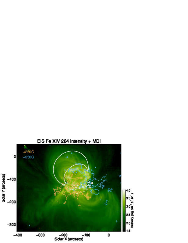
Fig. 7.3: EIS Fe xiv $264.78$Å intensity map. Orange (Turquoise) contours indicate a magnetic field strength of $+250\,({-250})\,\mathrm{G}$ in the simultaneous MDI magnetogram. Six white boxes are located at the position corresponding to those studied in Chapter 5. White lines rooted at those boxes indicate the magnetic field lines extrapolated from the magnetogram (see Appendix A).

We have discussed about several physical properties of each outflow region in Sections 7.4–7.7, and here some implications will be put on the coronal formation (i.e., heating) from the viewpoint of the outflows. The differences in those two outflow regions are listed in Table 7.1. The topology of magnetic field lines can be inferred from the extrapolated field lines (see Appendix A) and Doppler velocity maps obtained in Chapter 4 (Fig. 4.10). In order to confirm the connectivity of the magnetic field lines rooted at the studied outflow regions in Chapter 5, we drew projected field lines onto the intensity map of Fe xiv $264.78$Å as shown in Fig.7.3. The outflow regions U1–U6 are indicated by white boxes. The contours with orange (turquoise) indicate a magnetic field strength of $+250\,({-250})\,\mathrm{G}$ in the simultaneous MDI magnetogram.

Two solid white lines trace coronal loops, therefore we regarded the topology of the eastern outflow region as closed, which can be also seen as a coherent pattern tracing the coronal loops in the Doppler velocity maps. Four dashed white lines rooted at the western outflow region are connected to the opposite polarity around $(x,y)=(-160^{\prime\prime},-150^{\prime\prime})$, but the Doppler velocity maps clearly show that the blueshifted feature extends into the far west from which we suspected the topology of the western outflow region as open. The closed loops rooted at the eastern outflow region are brighter than the open structures extending from the western outflow region by one order of magnitude. This might reflect the length of each structure in the sense that the upflow easily fills a closed loop while it flows without obstacles in a open structure, which produces denser plasma in the closed loop.

As a consequence, it leads to the implication that the upflow from the bottom of the corona becomes dense in the closed loop because of the pressure balance between the corona and the transition region, which is consistent with our result that the electron density of EBW component was larger in the eastern region than in the western region (see Table 7.1). Although the difference in the electron density of the major component would not be trivial, the relationship of the column depth (i.e., larger $h_{\mathrm{Major}}$ in the eastern outflow region than in the western outflow region) may represent that the eastern outflow region consists of more coronal loops than the western outflow region.

We have evaluated mass leakage from the western outflow region in Section 7.7, however, the closed topology of the eastern outflow region may actually imply mass supply to the active region. If this is the case for a portion of the outflow region, it means that the outflow plays a crucial role in the coronal heating by supplying hot plasma into coronal loops. We suggest a possible picture in Fig. 7.4 as a summary of discussion in this chapter.

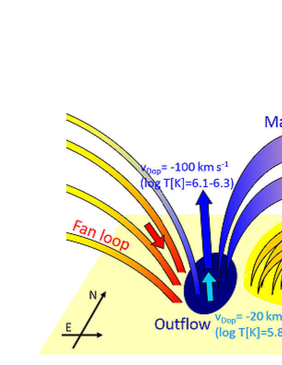
Fig. 7.4: Schematic picture of active region outflows.

7.9 Future work

The temporal evolution of outflow regions will be a different point of view from this thesis. Although a number of EIS scans revealed that the outflows are persistent for several days, it has not been clear how they evolve in the shorter timescale of $\sim\mathrm{min}$ because the scans usually take at least several hours to cover the whole active region. EIS has an observation mode to study the temporal variation of spectra (sit-and-stare mode) which tracks the same position on the Sun in accordance with the solar rotation. As examples of what are expected from such an observation, there are (1) identification of the origin in terms of the magnetic activity: if the outflows consist of elemental upflow events, we seek the signature of the driving magnetic activity at the photospheric level (e.g., shearing motion, coalescence, cancellation of magnetic patches), which is considered to be the underlying source of coronal dynamics, and (2) the evolution at different temperatures in response to the elemental upflows: this is useful to investigate the starting site (e.g., the upper transition region, higher up in the corona, etc.) which may be a clue to draw the geometry of the outflows.

In association with the first example of our expectation above, the motion of magnetic patches at the photosphere within a whole active region scale should be investigated. One approach is to study the flow field derived from the magnetograms through local correlation tracking (LCT) method which is feasible by using SOT and HMI magnetograms. Since the outflows are localized at the edge of active region core, there is a possibility that the flow field at the edge shows particular characteristics related to the outflows. It is also useful to construct the coronal magnetic field from consecutive magnetograms. The temporal evolution of coronal magnetic field lines connected to an outflow region can be studied from which we obtain the dynamical picture of the outflow region.

We will also aim to detect a signature of outflows by EUV imaging observations. A number of observations have been studied the propagating disturbances in fan loops observed by TRACE and SDO/AIA which are usually interpreted as waves or intermittent flows, however, the outflows themselves have not been observed in the images so far. Since the outflows are dark compared to fan loops which often exist in the neighbor, we must carefully exclude the location where the influence of fan loops is significant. The maximum of temperature response function of AIA $193$Å passband is $5\times 10^{-25}\,\mathrm{DN}\,\mathrm{cm}^{5}\,\mathrm{s}^{-1}\,\mathrm{pix}^{-1}$, which leads to the DN of $4$–$10^{3}$ with exposure time of $2\,\mathrm{s}$ (usual routine) and column emission measure of the outflow $n^{2}_{\mathrm{e}}h=10^{24.6\text{--}27.0}\,\mathrm{cm}^{-5}$ which was obtained in Chapter 5. That DN is enough for us to expect the detection of the outflows.

Chapter 8 Concluding remarks

We investigated the Doppler velocity and electron density of the outflows in NOAA AR10978 observed with the EUV Imaging Spectrometer (EIS) onboard Hinode.

In order to use the quiet region as a reference of the Doppler velocity, we analyzed the spectroscopic scans which cover the meridional line of the Sun and determined the Doppler velocity of emission lines with $5.7\leq\log T\,[\mathrm{K}]\leq 6.3$ in the quiet region for the first time (Chapter 3). It is shown that emission lines below $\log T\,[\mathrm{K}]=6.0$ have Doppler velocity of almost zero with an error of $1\text{--}3\,\mathrm{km}\,\mathrm{s}^{-1}$, while those above that temperature are blueshifted with gradually increasing magnitude: $v=-6.3\pm 2.1\,\mathrm{km}\,\mathrm{s}^{-1}$ at $\log T\,[\mathrm{K}]=6.25$. The Doppler velocity at $\log T\,[\mathrm{K}]=5.8$ was consistent with previous observations with SUMER within the estimated error. This analysis enabled us to determine a Doppler velocity from EIS spectra in the accuracy of $\leq 3\,\mathrm{km}\,\mathrm{s}^{-1}$, which was greatly improved from previous works where the accuracy was considered to be $\geq 5\,\mathrm{km}\,\mathrm{s}^{-1}$ (up to $10\,\mathrm{km}\,\mathrm{s}^{-1}$).

We measured the Doppler velocity of active region core, fan loops, and the outflow regions in NOAA AR10978 (Chapter 4) by using the velocity reference obtained in the previous chapter. While the Doppler velocity at active region core did not deviate much from that of the quiet region, other two structures exhibited characteristic behavior. Fan loops indicated $v\simeq 10\,\mathrm{km}\,\mathrm{s}^{-1}$ at $\log T\,[\mathrm{K}]=5.8$, declining to $v=-20\,\mathrm{km}\,\mathrm{s}^{-1}$ at $\log T\,[\mathrm{K}]=6.3$. In contrast to those fan loops, the outflow regions exhibited a blueshift corresponding to $v\simeq-20\,\mathrm{km}\,\mathrm{s}^{-1}$ at all temperature range below $\log T\,[\mathrm{K}]=6.3$, which implies that the plasma does not return to the solar surface at least in this temperature. The outflow regions have been sometimes regarded as identical to fan loops, however, we found the definitive difference of them in the Doppler velocity at the transition region temperature.

In Chapter 5, the electron density of the outflowing plasma was derived for the first time by using a density-sensitive line pair Fe xiv $264.78$Å/$274.20$Å. We extracted EBW component from the line profiles of Fe xiv through careful double-Gaussian fitting. Since those two emission lines are emitted from the same ionization degree of Fe ion, they should be shifted by the same amount of Doppler velocity, which required the simultaneous fitting of those two line profiles. We studied six locations selected from the eastern and western outflow regions. The average electron density in those six locations was $n_{\mathrm{Major}}=10^{9.16\pm 0.16}\,\mathrm{cm}^{-3}$ and $n_{\mathrm{EBW}}=10^{8.74\pm 0.29}\,\mathrm{cm}^{-3}$. The magnitude relationship between $n_{\mathrm{Major}}$ and $n_{\mathrm{EBW}}$ was different in the eastern and western outflow regions. We also calculated the column depth of each component in the line profiles, which leads to the results that (1) the outflows possess only a small fraction ($\sim 0.1$) compared the major rest component in the eastern outflow region, while (2) the outflows dominate over the rest plasma by a factor of around five in the western outflow region. The coronal structures beside those outflow regions show different appearance: loops connected to the opposite magnetic polarities at the eastern outflow regions, and only diffuse structures extending away from the active region, which might affect the density and column depth of the outflows.

We developed a new method in line profile analysis to investigate the electron density of EBW component in Chapter 6, which we refer to as $\lambda$-$n_{\mathrm{e}}$ diagram. This method has an advantage that it is independent from the fitting model. By using $\lambda$-$n_{\mathrm{e}}$ diagram, we confirmed that EBW component in Fe xiv line profiles has smaller electron density than that of the major component at the western outflow region.

We discussed the implications from our results in Chapter 7. The outflow regions and fan loops, which has been often discussed in the same context, exhibited different temperature dependence of Doppler velocity. We concluded these structures are not identical (Section 7.3). We tried to interpret the outflows in terms of the siphon flow along coronal loops, but it turned out to be unreasonable (Section 7.4). The temperature dependence of the Doppler velocity in the outflow regions obtained in Chapter 4 were different from that was predicted by a numerical simulation (Patsourakos & Klimchuk 2006), which dealt with impulsive heating with longer timescale than the cooling (Section 7.5.1). As for the case if intermittent heating is responsible for the outflows, the duration of heating was crudely estimated to be longer than $\tau=500\,\mathrm{s}$ for the energy input of $10^{24}\,\mathrm{erg}$ (i.e., nanoflare) so that the density of upflows from the footpoints becomes compatible with that of the observed outflows (Section 7.5.2). The electron density and column depth of the upflows in the eastern and western outflow regions were different, which was considered to be due to the magnetic structure above the outflow regions. The mass leakage occurs at the western outflow region (small $n_{\mathrm{EBW}}$ and large $h_{\mathrm{EBW}}$), on the other hand, there is a possibility of the mass supply to active region loops at the eastern outflow region (large $n_{\mathrm{EBW}}$ and small $h_{\mathrm{EBW}}$), which may be related to the coronal heating process (Section 7.8).

In order to reveal the nature of active region outflows further, we proposed several targets: (1) temporal evolution of the outflows in a short timescale of $\sim\mathrm{min}$ for seeking the signature of drivers, (2) flow field in the photospheric magnetograms for investigating the dynamic topology above the outflow regions, and (3) moving feature in EUV images for detecting the outflows and related phenomena morphologically.

Appendix A Morphology of the outflow region

A.1 Introduction

We study the magnetic field around the outflow region using a magnetogram taken by SoHO/MDI in this chapter. The configuration of the magnetic field helps us to infer the 3D structure of the plasma flow in the corona. The outflow region has been said to be located at the region where magnetic topology switches and the lengths of coronal loops change drastically (Baker et al. 2009). In this chapter, the potential magnetic field in the corona around NOAA AR10978 was constructed from an MDI magnetogram at the photosphere through Green’s function method (Sakurai 1982). The purpose is to study the connectivity of magnetic field lines rooted at the outflow region studied in this thesis.

MDI is an instrument onboard SoHO which measures the continuum intensity, Doppler velocity, and line-of-sight magnetic field strength of the whole Sun (Scherrer et al. 1995). Those observables are derived by processing the spectrum of an absorption line Ni i $6768$Å. The magnetic field is measured by using the Zeeman splitting. The FOV of MDI is routinely set to the whole Sun, and MDI takes a magnetogram every $96\,\mathrm{min}$ ($15$ images per day). The spatial resolution of MDI is $\simeq 4^{\prime\prime}$ (pixel size of $1^{\prime\prime}.98$). In this chapter, we used a magnetogram around NOAA AR10978 when it passes near the center of the solar disk.

We have measured Doppler velocity and electron density of the outflow region in previous chapters by analyzing the spectra obtained with Hinode/EIS, which cannot be achieved by filter imagers. However, a spectroscopic scan with EIS usually takes several hours to complete scanning a whole active region (size of $\sim 200^{\prime\prime}$) with normal exposure time of $\gtrsim 30\,\mathrm{s}$. It has been reported that the outflow continues for the timescale of several days (Bryans et al. 2010; Démoulin et al. 2013). This means that the global structure of the outflow region should have been captured by current EIS data while some phenomena with short duration which might form the outflow were missed.

In order to seek such a signature which might be associated with the outflow, we analyze EUV images taken by SoHO/EIT and TRACE. EIT is an EUV telescope onboard SoHO which routinely takes a whole solar image every $12\,\mathrm{min}$. The spatial resolution of EIT is $\sim 5^{\prime\prime}$ (pixel size of $2^{\prime\prime}.6$), which is rather coarse. However, it is useful when we align an MDI magnetogram with EUV images taken by other telescopes, since MDI and EIT are well coaligned by referring the solar limb. TRACE has a spatial resolution of $\sim 1^{\prime\prime}$ (pixel size of $0^{\prime\prime}.50$) which is higher than that of EIS (i.e., $2$–$3^{\prime\prime}$) so that it is useful to study the morphology of the outflow region. The temporal cadence of TRACE images used here was roughly $1\,\mathrm{min}$, which is much better than that of the EIS scan. Previous observations have revealed that the outflow emanated from dark region outside the active region core (Doschek et al. 2008), but since it has not been revealed whether any activities are occurring in the site. We aim to detect some signatures which might be linked to the outflow.

A.2 Potential field extrapolation from an MDI magnetogram

Coronal magnetic field plays a dominant role in the sense that the plasma is structured by the magnetic field (e.g., coronal loops), while motion across the field is hindered. The coronal plasma is confined to magnetic field lines due to its small Larmor radius: $\simeq 2\,\mathrm{cm}$ for electrons and $\simeq 1\,\mathrm{m}$ for protons in the typical coronal environment ($T=10^{6}\,[\mathrm{K}]$ and $B=10\,[\mathrm{G}]$). Therefore, the motion of the coronal plasma can be approximately considered to as one dimensional along the magnetic field, which helps us to implicate dynamical picture of the corona.

However, direct measurement of the coronal magnetic field has been under developing and there are only a few measurements around an active region by an infrared emission line (Lin et al. 2004) and radio spectrum (Gary & Hurford 1994). As an alternative way, the magnetic field in the corona can be inferred through the extrapolation of a photospheric magnetogram into the corona. Here we adopted the potential field calculation (Schmidt 1964; Sakurai 1982) in order to extrapolate an MDI magnetogram at the photosphere around NOAA AR10978.

A.2.1 Calculation method

The plasma beta in the corona is considered to be much less than unity ($\beta\ll 1$), which means that the Lorentz force dominates the gas pressure gradient, thus,

$$\left(\nabla\times\bm{B}\right)\times\bm{B}=\bm{0}$$ (A.1)

holds in the static equilibrium, where $\bm{B}$ is the magnetic field. This equation is nonlinear in general, but it becomes rather simple in the lowest order approximation like

$$\nabla\times\bm{B}=\bm{0}\,\text{,}$$ (A.2)

which means that the electric current is zero everywhere in the corona. In this case, the magnetic field $\bm{B}$ can be represented as $\bm{B}=-\nabla\phi(\bm{r})$ where $\phi(\bm{r})$ is a potential function. Then Eq. (A.2) becomes

$$\nabla^{2}\phi(\bm{r})=0\mspace{18.0mu}(z>0)\,\text{,}$$ (A.3)

which is the Laplace equation. A magnetogram at the photosphere plays a role as a boundary condition (e.g., Neumann problem), and it can be written as

$$-\bm{n}\cdot\nabla\phi(\bm{r})=B_{\mathrm{ph}}(x,y,0)\mspace{18.0mu}(z=0)\,\text{,}$$ (A.4)

where $\bm{n}$ is a normal vector as to the solar surface, and $B_{\mathrm{ph}}$ is the vertical magnetic strength obtained at the photosphere ($z=0$). The $z$ direction was set to be toward the observer.

Here we used the Green’s function method to solve Eq. (A.3) with the boundary condition represented by Eq. (A.4) (Sakurai 1982; classical Schmidt method). If we found a function $G(\bm{r},\bm{r}^{\prime})$ which satisfies the following three conditions:

$$\nabla^{2}G(\bm{r},\bm{r}^{\prime})=0 (z>0)\,\text{,}$$ (A.5)

$$G(\bm{r},\bm{r}^{\prime})\longrightarrow 0 (\left|\bm{r}-\bm{r}^{\prime}\right|\rightarrow\infty;z>0)\,\text{,}$$ (A.6)

$$-\bm{n}\cdot\nabla G(\bm{r},\bm{r}^{\prime})=\delta(x-x^{\prime})\delta(y-y^{\prime}) (z=0)\,\text{,}$$ (A.7)

the potential function $\phi$ can be represented by

$$\phi(\bm{r})=\int B_{\mathrm{ph}}(\bm{r}^{\prime})G(\bm{r},\bm{r}^{\prime})dS^{\prime}\,\text{,}$$ (A.8)

where $\delta(x-x^{\prime})$ and $\delta(y-y^{\prime})$ are the Dirac’s delta function. The term $dS^{\prime}$ indicates an area element in $x$–$y$ plane. It is easy to prove that Eq. (A.8) satisfies the boundary condition Eq. (A.4). The function $G(\bm{r},\bm{r}^{\prime})$ is called the Green’s function and here has a functional form of

$$G(\bm{r},\bm{r}^{\prime})=\dfrac{1}{2\pi\left|\bm{r}-\bm{r}^{\prime}\right|}\,\text{.}$$ (A.9)

From this expression, the potential function can be calculated by Eq. (A.8), then, magnetic field strength at any locations will be derived from $\bm{B}=-\nabla\phi(\bm{r})$. The integral in Eq. (A.8) was replaced by the summation of discretized data points in the practical calculation.

A.2.2 Properties of calculated field lines

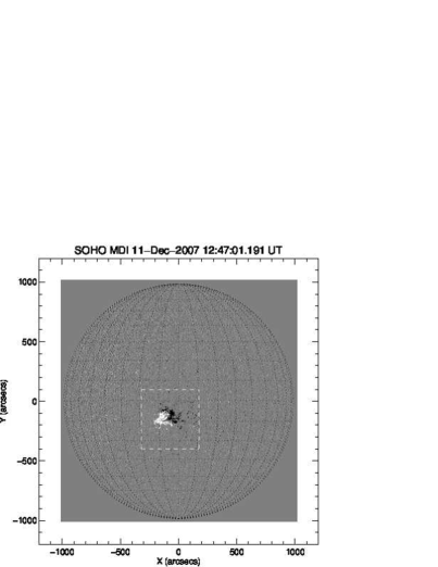
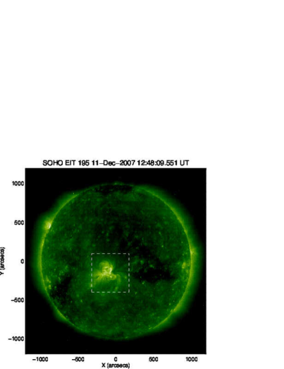
Fig. A.1: Left: MDI magnetogram taken on 2007 December 11 12:47:01UT. Right: EIT image taken on 2007 December 11 12:48:09UT. White dashed lines in each panel indicate the calculation box for potential field.

We applied the potential field extrapolation to an MDI magnetogram taken on 2007 Dec 11, which is shown in Fig. A.1. Left and Right panels respectively indicate an MDI magnetogram and an EIT image obtained almost simultaneously. The area including the active region NOAA AR10978 was extracted near the disk center around $(x,y)=(-150,-100)$ which is shown by white dashed square, so that we could neglect the effect of the curvature of the solar surface ($\cos\theta\gtrsim 0.97$, $\theta$ is an angle between our line of sight and the normal vector at the solar surface). The size of the calculated box was $250\times 250\times 200\,\mathrm{pix}^{3}$ ($500^{\prime\prime}\times 500^{\prime\prime}\times 400^{\prime\prime}$), which is large enough to include whole active region, and the magnetic field was calculated in the orthogonal coordinate.

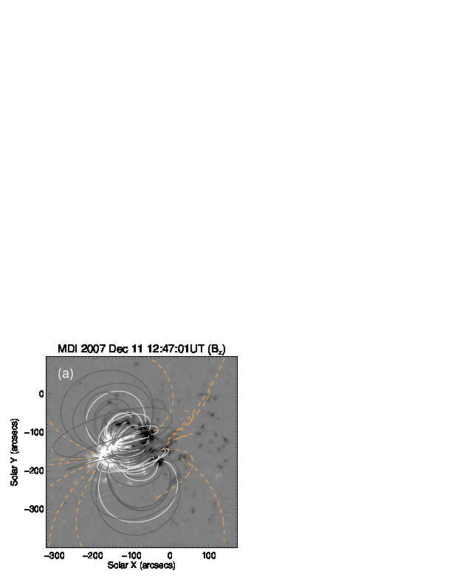
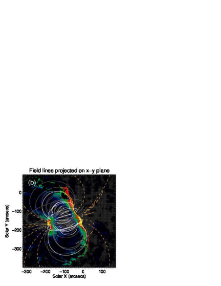
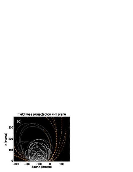
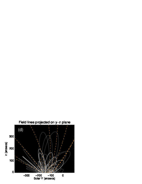
Fig. A.2: Magnetic field extrapolated by the potential calculation using Green’s function method described in Sakurai (1982). (a) Magnetogram at $z=0$ obtained by SoHO/MDI. (b) Calculated field lines projected onto $x$–$y$ plane. White (Gray) lines indicated that the magnetic field strength at their footpoint is larger than $500$ $(200)\,\mathrm{G}$. Orange dashed lines indicate that the field line goes out from the side boundary. Background color shows the length of field lines rooted at each pixel. Gray hatched region indicate that field lines rooted at the pixels penetrate into the side boundary or the top of the calculation box ($500^{\prime\prime}\times 500^{\prime\prime}\times 400^{\prime\prime}$). (c) Calculated field lines projected onto $x$–$z$ plane. (d) Calculated field lines projected onto $y$–$z$ plane.

The result of the potential field extrapolation is shown in Fig. A.2. The location $(x,y)$ are defined by heliocentric coordinates in which $y$ lies in the rotational axis of the Sun (positive value means north), and $z$ is in the direction vertical to the solar surface. Panels respectively show calculated field lines projected onto (a) the magnetogram at $z=0$, (b) $x$–$y$ plane, (c) $x$–$z$ plane, and (d) $y$–$z$ plane. For panel (a) and (b), white (gray) lines indicated that the magnetic field strength at their footpoint is larger than $500$ $(200)\,\mathrm{G}$. Orange dashed lines indicate that the field line goes out from the side boundary or the top of the calculation box. Background color in panel (b) shows the length of field lines rooted at each pixel. Gray hatched region indicate that field lines rooted at the pixels penetrate into the side boundary or the top of the calculation box. AR10978 had a leading negative sunspot around $(x,y)=(-30^{\prime\prime},-180^{\prime\prime})$ and following positive region less concentrated, which can be seen in panel (a). The loop structures connecting those opposite polarities are prominent as shown by white/gray field lines in panels (a) and (b). The field lines rooted at the region of strong magnetic field strength ($B_{z}\geq 500\,\mathrm{G}$) reach the height up to $\sim 200\,\mathrm{Mm}$ in the maximum as shown in panels (c) and (d).

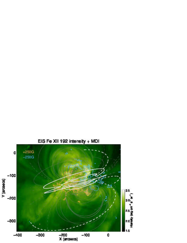
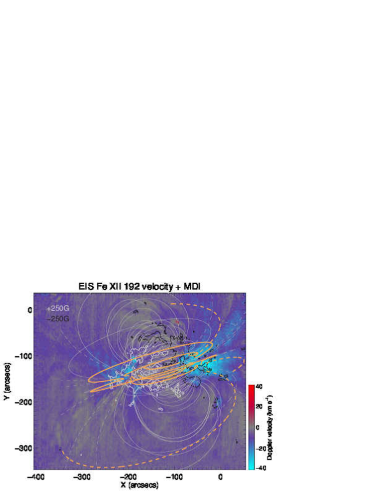
Fig. A.3: Left: EIS Fe xii $192.39$Å intensity and potential field calculated from MDI magnetogram. Right: EIS Fe xii $192.39$Å Doppler velocity and potential field calculated from MDI magnetogram. Dashed lines indicate that the field line goes out from the boundary of the calculation box of potential field. White/Orange thick lines show the field line rooted at the outflow region.

In order to see the correspondence between magnetic field and coronal structures more clearly, the calculated field lines were projected on the EIS Fe xii $192.39$Å intensity (left) and Doppler velocity (right) map as shown in Fig. A.3. Gray solid (dashed) lines indicate the field line closed within (goes out from) the calculation box. In the intensity map, it is clearly seen that the legs of two fan loops extending to the south east well coincide with the projected gray dashed lines. At the west region of the active region, the blueshifted area has a shape which is well traced by the projected gray dashed lines as shown in the Doppler velocity map. The loop structures connecting the opposite polarities near the core are not clearly seen in the formation temperature of Fe xii, however, those are prominent in Fe xvi intensity map (cf. panel f in Fig. 4.3).

White/Orange thick lines are the loops rooted in the outflow region at their western footpoints. The lengths of these loops were $\geq 100\,\mathrm{Mm}$. The inclination angle of those at their footpoint as to the solar surface was $30$–$50\,\mathrm{deg}$. Potential field extrapolation clearly show that some of the field lines rooted in the outflow region were not long enough to reach the heliosphere but rather compact ($100$–$200\,\mathrm{Mm}$ in the height). The opposite footpoints of those field lines are located at the neighbor of the east edge of the core region (i.e., closed loop), and they look slightly being inside the edge. Other field lines rooted in the outflow region are connected to the eastern outflow region, and the rest loops are so long enough to go out from the calculation box.

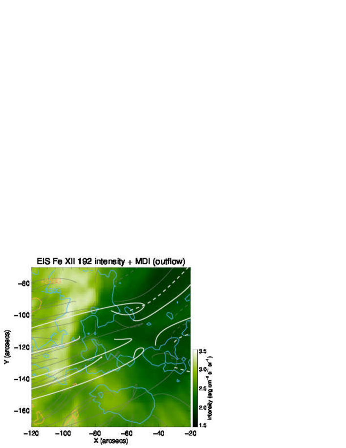
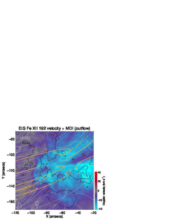
Fig. A.4: Zoomed outflow region as same format as Fig. A.3.

Fig. A.4 shows the zoomed outflow region as same format as Fig. A.3. We drew the orange/white thick lines from the locations where the upflow speed is large as seen in lower panel. There are not spatial correspondence between the Doppler velocity and the magnetic field strength at the photosphere (black contour: $-250\,\mathrm{G}$). The blueshifted region prevails more homogeneously than the magnetic field strength. This might be caused by the line-of-sight integration. Since almost all magnetic field lines have an inclination from the normal to the solar surface, the upflowing plasma at certain height in a coronal loop is not magnetically connected to the photospheric level along the same line of sight.

A.3 EUV imaging observations

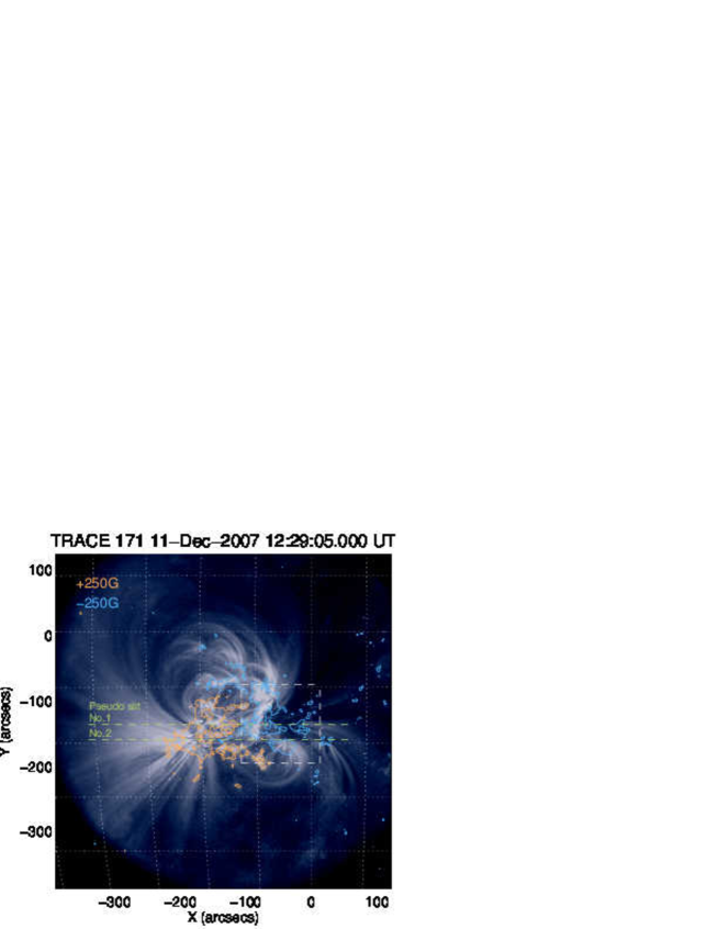
Fig. A.5: A TRACE image taken on 2007 December 11 12:29:05UT. Orange (Blue) contours indicate the magnetic field strength of $+250$ ($-250$) $\mathrm{G}$ in MDI magnetogram. A white dashed square shows the region zoomed in Fig. A.6. Two horizontal green dashed lines indicate pseudo slits for $x$-$t$ diagrams shown in Fig. A.7.

TRACE took EUV image of NOAA AR10978 mainly through the $171$Å passband on 2007 December 11. This passband includes dominant contribution from Fe ix/x emission lines and their formation temperature is $\log T\,[\mathrm{K}]=5.9$–$6.0$. Fig. A.5 shows a TRACE $171$Å image taken at 12:29:05UT. It is clearly seen that multiple loop system connects between positive polarity (orange contour) and negative polarity (turquoise contour), and fan loops extend out of the FOV at the both sides as more prominent in the east than in the west. Note that the outflow region focused in this thesis corresponds to the dark location within the white dashed box where the magnetic field strength reaches several hundred Gauss.

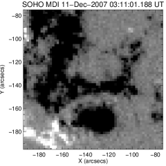
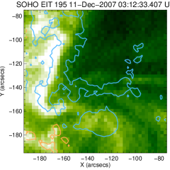
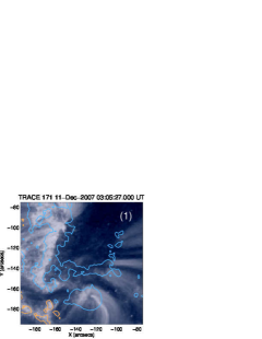
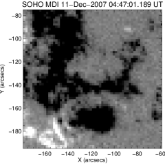
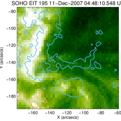
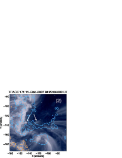
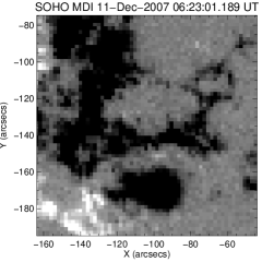
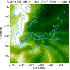
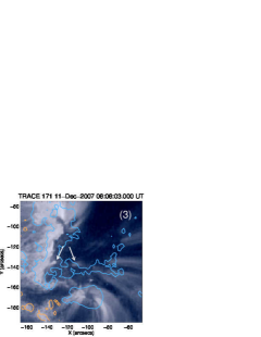
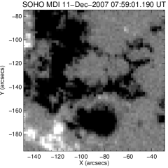
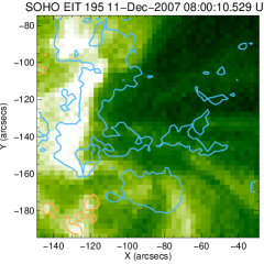
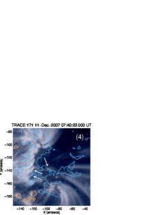
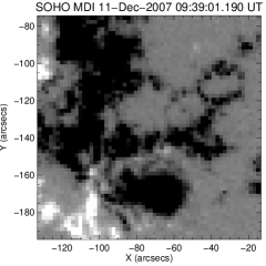
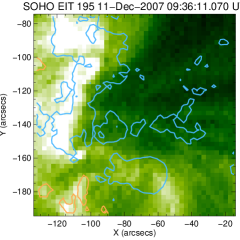
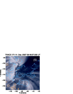
Fig. A.6: Magnetogram and EUV images of the outflow region on 2007 December 11 during around 3–20UT. Left column: MDI magnetograms. Middle column: EIT $195$Å images. Right column: TRACE $171$Å images.

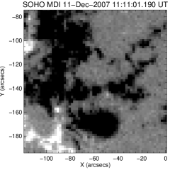
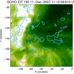
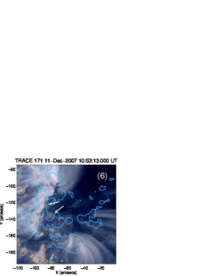
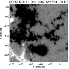
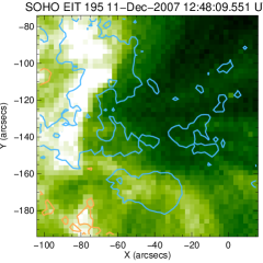
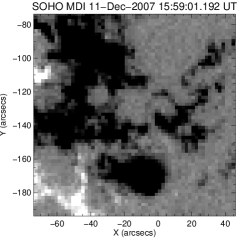
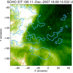
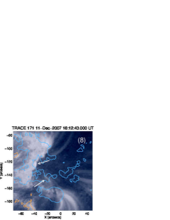
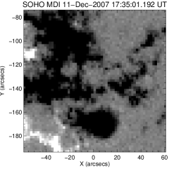
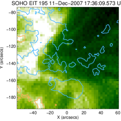
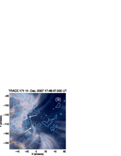
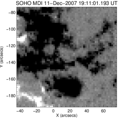
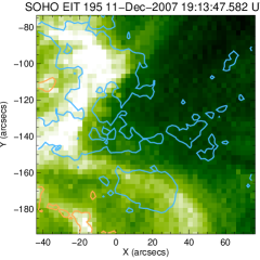
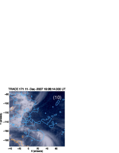
Fig. A.6: Continued.

In Fig. A.6, we show consecutive images taken by MDI (left column), EIT $195$Å passband (middle column), and TRACE $171$Å passband (right column) with the FOV indicated by the white dashed box in Fig. A.5. Time intervals between each row are $\sim 96\,\mathrm{min}$ (temporal cadence of MDI observations). Colored contours in EIT images (middle column) and TRACE images (right column) show $+250\,\mathrm{G}$ (orange contour) and $-250\,\mathrm{G}$ (turquoise contour) on each MDI magnetogram (left column) which was taken at near timing. As seen in the MDI magnetograms, there is a negative sunspot at the bottom of panels from which coronal loops extend to the south in EIT and TRACE images. An arc-like pattern lies at the north of the sunspot in MDI magnetograms (above $y=-150^{\prime\prime}$). From left hand side of the arc-like structure, multiple loops system extends to the opposite polarity at the east, while there is no corresponding distinct loops at the bottom side of the arc-like structure. The right hand side of the arc-like structure seems to be footpoints of fan loops extending to the west direction. The multiple loop system exists only at the east half of the left hand side of that structure during $3$–$12$UT as especially seen in TRACE images. The overall structure in magnetograms did not change much.

A careful inspection at the TRACE images leads to the detection of intermittent appearance of some bright structures as indicated by white arrows in Fig. A.6. There are two types of structures: one is a coronal loop which forms the multiple loop system connecting positive and negative polarities (e.g., a left arrow in the second and third rows from the upper), while the other is extended toward relatively outside (e.g., a right arrow in the second and third rows). Note that the area possessed by these small bright structures are not dominant in the outflow region.

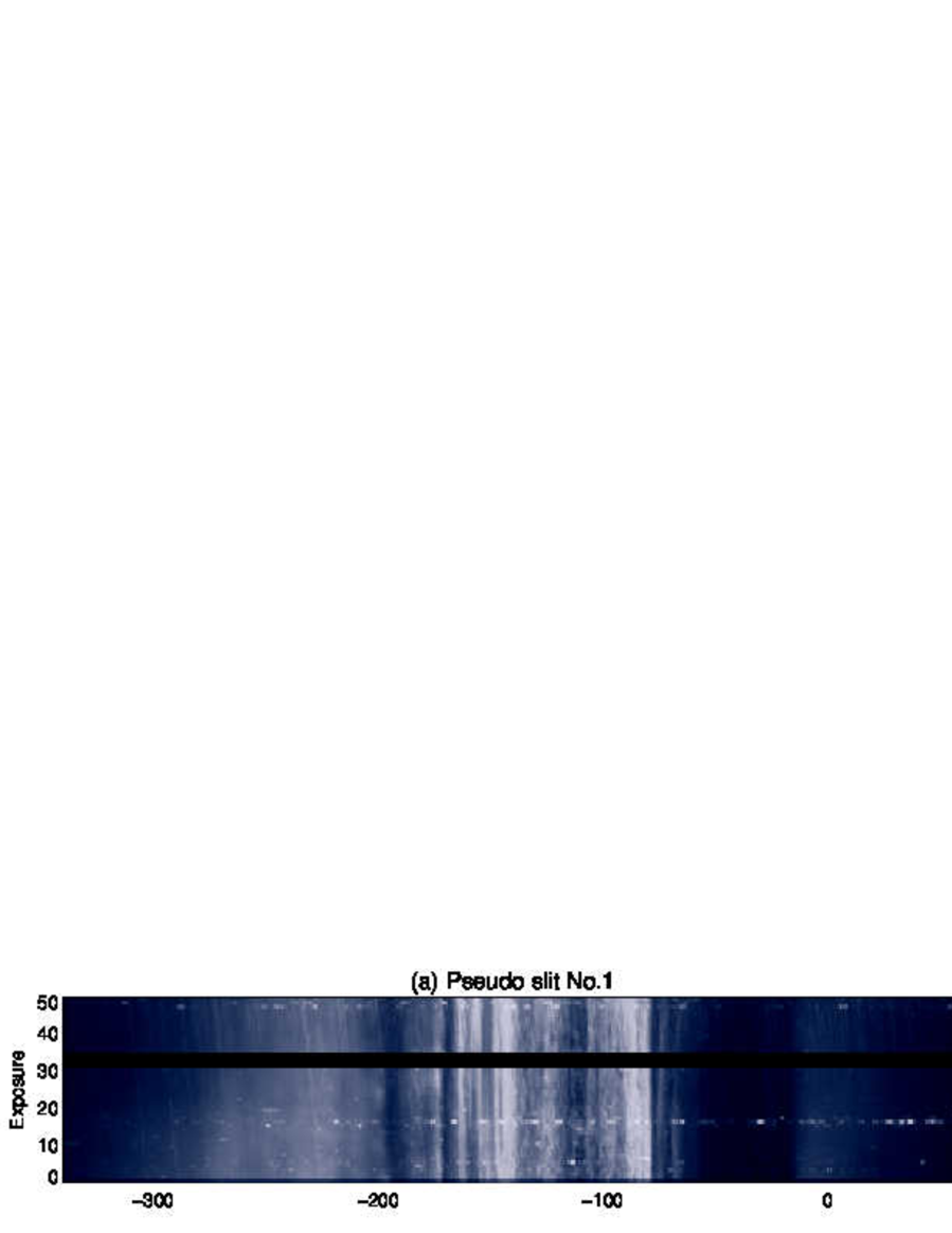
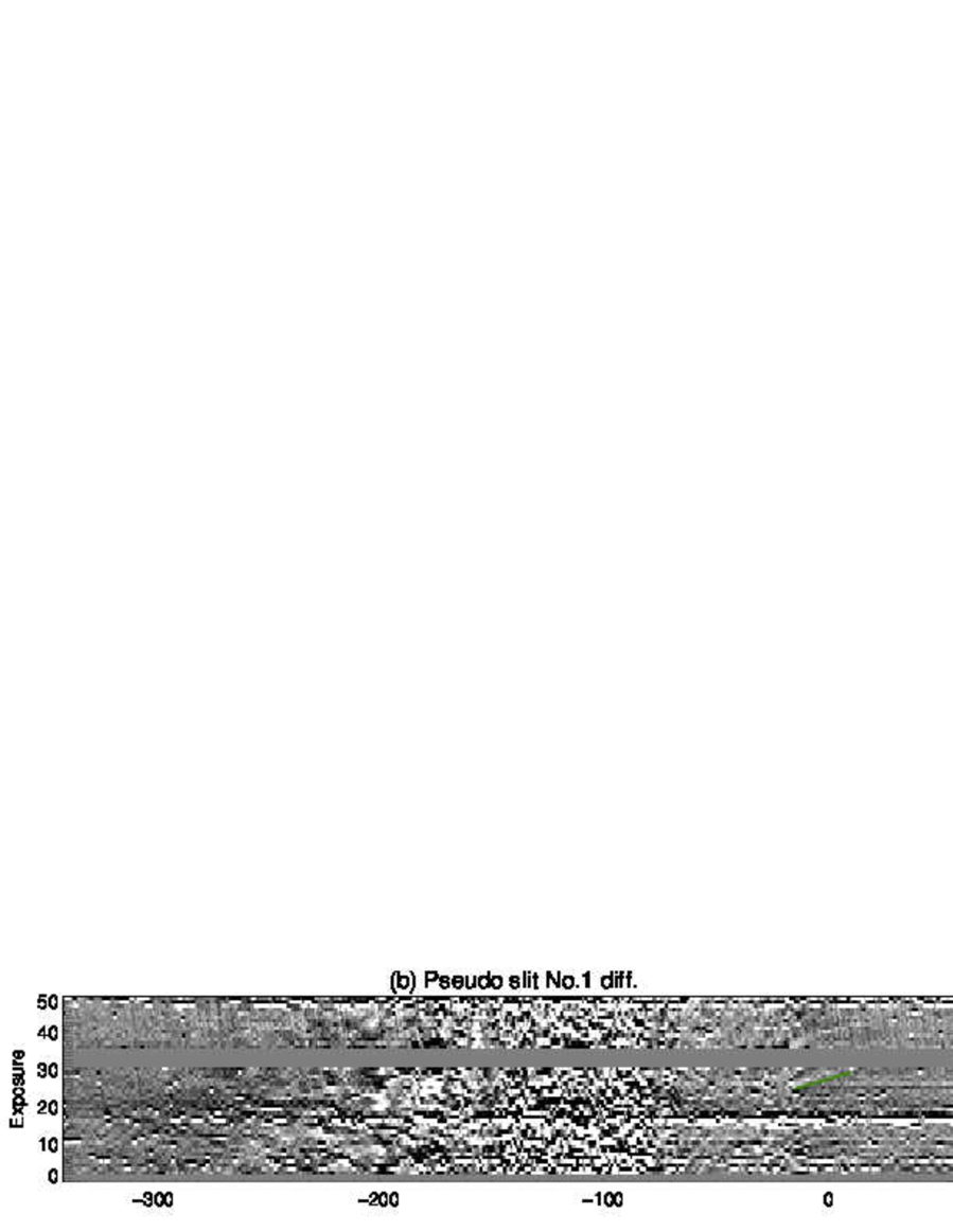
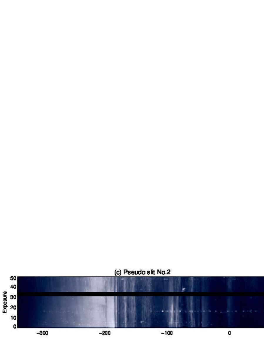
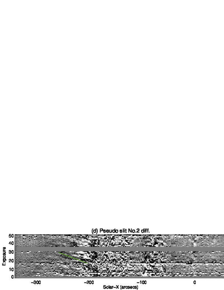
Fig. A.7: $x$-$t$ diagrams for pseudo slits indicated by horizontal green dashed lines in Fig. A.5. Each panel shows $x$-$t$ diagram for (a) intensity at pseudo slit No.1, (b) running difference at pseudo slit No.1, (c) intensity at pseudo slit No.2, and (d) running difference at pseudo slit No.2. A Green thick line in each panel indicates the propagating disturbance traced visually.

Fig. A.7 shows $x$-$t$ diagrams made at horizontal green dashed lines in the TRACE map (Fig. A.5). We selected the observational sequence during 2007 December 11 12:29–13:32UT when it observed the active region with a temporal cadence of $\sim 1\,\mathrm{min}$ and the least gap in time. The pseudo slits have a width of $5\,\mathrm{pix}$ so that the signal-to-noise ratio would be improved. The location of the pseudo slit was set in each image so that it continuously tracks the same region since the solar rotates about $15^{\prime\prime}$ ($30\,\mathrm{pixels}$) during the TRACE observation. Panels (a) and (c) respectively show an $x$-$t$ diagram for the intensity at the pseudo slit No.1 and No.2. The horizontal (vertical) axis shows the solar $X$ and exposure No. (intervals of roughly $1\,\mathrm{min}$, but not exactly constant). The unit of the intensity is normalized by the median at each exposure because we found that the mean intensity increases with time during the observation, which might be a result of the gradual change in the telescope environment. Panels (b) and (d) show the running differences in temporal direction. Note that sharp patterns slightly inclined to $-x$ direction (from right bottom to left upper), which are clearly seen around $x=-300^{\prime\prime}\,\text{--}\,{-200^{\prime\prime}}$, may be due to the instrumental effect (e.g., CCD characteristics). We found these patterns were located at specific pixels on CCD. The black region (exposure No.$31$–$34$) means that there is a time gap of a few minutes.

The pseudo slit No.1 cuts across the center portion of the active region core, the outflow region, and goes through a fan loop extending toward the west. The slit also cut fan loops at the east edge of the core, but it was not aligned along the fan loops. The pseudo slit No.2 was set to cut along the fan loops at the east edge. We can see several propagating features from the footpoints of fan loops: $x=-15^{\prime\prime}$ to $10^{\prime\prime}$ in panel (b) and $x=-200^{\prime\prime}$ to $-260^{\prime\prime}$ in panel (d) as indicated by green lines. These propagating disturbances occurred not only once but repetitively, and are considered to be identical to those observed by previous TRACE observations (De Moortel et al. 2000; Winebarger et al. 2001). In contrast to fan loops, the outflow region ($x=-80^{\prime\prime}\,\text{--}\,-20^{\prime\prime}$ in panel a and b) did not exhibit any clear propagating features in the analyzed data. We also tried to seek signatures by looking into the TRACE movie, however, we could not detect the prominent flow pattern.

A.4 Summary

The magnetic field above the active region NOAA AR10978 was extrapolated from an MDI magnetogram through solving the Laplace equation by Green’s function method. The magnetogram was taken near at the disk center and we calculated the magnetic field in the orthogonal coordinate. The size of the calculation box was enough large to include the whole active region ($500^{\prime\prime}\times 500^{\prime\prime}\times 400^{\prime\prime}$). The extrapolated field lines are in well coincidence with the morphology of EUV loops seen in the EIS intensity and Doppler velocity maps.

The field lines rooted at the outflow region had lengths of $\simeq 100$–$200\,\mathrm{Mm}$ and their footpoints with the opposite polarity were located slightly inside the east edge of the active region. While a part of the calculated field lines corresponding to fan loops went out from the calculation box from its side or top boundary, those rooted at the outflow region were not so long enough to reach higher than $\simeq 200\,\mathrm{Mm}$, which means rather “closed” field lines.

EUV images taken by SoHO/EIT and TRACE showed that the magnetic field strengths at the outflow region were relatively strong ($\lvert B_{z}\rvert\geq 200\,\mathrm{G}$). A careful inspection at the TRACE images helped us to find the intermittent appearance of some bright structures which looked like a leg of coronal loops emanated from the outflow region. However, these intermittent phenomena obviously did not possess dominant area in the outflow region, which may indicate that those are not a main contributor to the outflow. The $x$-$t$ diagrams clearly showed propagating disturbances in fan loops as reported by previous observations, however, we could not detect the prominent flow pattern in the outflow region.

References

- Aschwanden et al. (2000) Aschwanden, M. J., Nightingale, R. W., & Alexander, D. 2000, ApJ, 541, 1059
- Baker et al. (2009) Baker, D., van Driel-Gesztelyi, L., Mandrini, C. H., Démoulin, P., & Murray, M. J. 2009, ApJ, 705, 926
- Berger et al. (1999) Berger, T. E., de Pontieu, B., Fletcher, L., et al. 1999, Sol. Phys., 190, 409
- Bradshaw (2008) Bradshaw, S. J. 2008, A&A, 486, L5
- Bradshaw et al. (2011) Bradshaw, S. J., Aulanier, G., & Del Zanna, G. 2011, ApJ, 743, 66
- Brooks & Warren (2011) Brooks, D. H., & Warren, H. P. 2011, ApJL, 727, L13
- Brooks & Warren (2012) —. 2012, ApJL, 760, L5
- Brown et al. (2007) Brown, C. M., Hara, H., Kamio, S., et al. 2007, PASJ, 59, 865
- Bryans et al. (2010) Bryans, P., Young, P. R., & Doschek, G. A. 2010, ApJ, 715, 1012
- Cargill & Priest (1980) Cargill, P. J., & Priest, E. R. 1980, Sol. Phys., 65, 251
- Chae et al. (1998) Chae, J., Yun, H. S., & Poland, A. I. 1998, ApJS, 114, 151
- Culhane et al. (2007) Culhane, J. L., Harra, L. K., James, A. M., et al. 2007, Sol. Phys., 243, 19
- Dadashi et al. (2012) Dadashi, N., Teriaca, L., Tripathi, D., Solanki, S. K., & Wiegelmann, T. 2012, A&A, 548, A115
- De Moortel et al. (2000) De Moortel, I., Ireland, J., & Walsh, R. W. 2000, A&A, 355, L23
- De Pontieu et al. (2009) De Pontieu, B., McIntosh, S. W., Hansteen, V. H., & Schrijver, C. J. 2009, ApJL, 701, L1
- De Pontieu et al. (2011) De Pontieu, B., McIntosh, S. W., Carlsson, M., et al. 2011, Science, 331, 55
- Del Zanna (2008) Del Zanna, G. 2008, A&A, 481, L49
- Del Zanna et al. (2011) Del Zanna, G., Aulanier, G., Klein, K.-L., & Török, T. 2011, A&A, 526, A137
- Démoulin et al. (2013) Démoulin, P., Baker, D., Mandrini, C. H., & van Driel-Gesztelyi, L. 2013, Sol. Phys., 283, 341
- Dere et al. (1997) Dere, K. P., Landi, E., Mason, H. E., Monsignori Fossi, B. C., & Young, P. R. 1997, A&AS, 125, 149
- Doschek (2012) Doschek, G. A. 2012, ApJ, 754, 153
- Doschek et al. (2008) Doschek, G. A., Warren, H. P., Mariska, J. T., et al. 2008, ApJ, 686, 1362
- Edlén (1943) Edlén, B. 1943, ZA, 22, 30
- Gary & Hurford (1994) Gary, D. E., & Hurford, G. J. 1994, ApJ, 420, 903
- Golub et al. (2007) Golub, L., Deluca, E., Austin, G., et al. 2007, Sol. Phys., 243, 63
- Hansteen et al. (2010) Hansteen, V. H., Hara, H., De Pontieu, B., & Carlsson, M. 2010, ApJ, 718, 1070
- Hara et al. (2008) Hara, H., Watanabe, T., Harra, L. K., et al. 2008, ApJL, 678, L67
- Harra et al. (2008) Harra, L. K., Sakao, T., Mandrini, C. H., et al. 2008, ApJL, 676, L147
- Kamio et al. (2010) Kamio, S., Hara, H., Watanabe, T., Fredvik, T., & Hansteen, V. H. 2010, Sol. Phys., 266, 209
- Klimchuk (2012) Klimchuk, J. A. 2012, Journal of Geophysical Research (Space Physics), 117, 12102
- Korendyke et al. (2006) Korendyke, C. M., Brown, C. M., Thomas, R. J., et al. 2006, Appl. Opt., 8674
- Kosugi et al. (2007) Kosugi, T., Matsuzaki, K., Sakao, T., et al. 2007, Sol. Phys., 243, 3
- Landi et al. (2012) Landi, E., Del Zanna, G., Young, P. R., Dere, K. P., & Mason, H. E. 2012, ApJ, 744, 99
- Lin et al. (2004) Lin, H., Kuhn, J. R., & Coulter, R. 2004, ApJL, 613, L177
- McIntosh & De Pontieu (2009) McIntosh, S. W., & De Pontieu, B. 2009, ApJL, 706, L80
- McIntosh et al. (2012) McIntosh, S. W., Tian, H., Sechler, M., & De Pontieu, B. 2012, ApJ, 749, 60
- Murray et al. (2010) Murray, M. J., Baker, D., van Driel-Gesztelyi, L., & Sun, J. 2010, Sol. Phys., 261, 253
- Nishizuka & Hara (2011) Nishizuka, N., & Hara, H. 2011, ApJL, 737, L43
- Parker (1958) Parker, E. N. 1958, ApJ, 128, 664
- Patsourakos & Klimchuk (2006) Patsourakos, S., & Klimchuk, J. A. 2006, ApJ, 647, 1452
- Patsourakos & Klimchuk (2013) —. 2013, 6th Coronal Loops Workshop, presentation
- Peter (1999) Peter, H. 1999, ApJ, 516, 490
- Peter (2010) —. 2010, A&A, 521, A51
- Peter & Judge (1999) Peter, H., & Judge, P. G. 1999, ApJ, 522, 1148
- Rosner et al. (1978) Rosner, R., Tucker, W. H., & Vaiana, G. S. 1978, ApJ, 220, 643
- Roussel-Dupré & Shine (1982) Roussel-Dupré, D., & Shine, R. A. 1982, Sol. Phys., 77, 329
- Sakao et al. (2007) Sakao, T., Kano, R., Narukage, N., et al. 2007, Science, 318, 1585
- Sakurai (1982) Sakurai, T. 1982, Sol. Phys., 76, 301
- Scherrer et al. (1995) Scherrer, P. H., Bogart, R. S., Bush, R. I., et al. 1995, Sol. Phys., 162, 129
- Schmidt (1964) Schmidt, H. U. 1964, NASA Special Publication, 50, 107
- Serio et al. (1981) Serio, S., Peres, G., Vaiana, G. S., Golub, L., & Rosner, R. 1981, ApJ, 243, 288
- Storey et al. (2000) Storey, P. J., Mason, H. E., & Young, P. R. 2000, A&AS, 141, 285
- Swings (1943) Swings, P. 1943, ApJ, 98, 116
- Tayal (2008) Tayal, S. S. 2008, ApJS, 178, 359
- Teriaca et al. (1999) Teriaca, L., Banerjee, D., & Doyle, J. G. 1999, A&A, 349, 636
- Tian et al. (2011) Tian, H., McIntosh, S. W., De Pontieu, B., et al. 2011, ApJ, 738, 18
- Tsuneta et al. (2008) Tsuneta, S., Ichimoto, K., Katsukawa, Y., et al. 2008, Sol. Phys., 249, 167
- Ugarte-Urra & Warren (2011) Ugarte-Urra, I., & Warren, H. P. 2011, ApJ, 730, 37
- Warren et al. (2011) Warren, H. P., Ugarte-Urra, I., Young, P. R., & Stenborg, G. 2011, ApJ, 727, 58
- Winebarger et al. (2001) Winebarger, A. R., DeLuca, E. E., & Golub, L. 2001, ApJL, 553, L81
- Withbroe & Noyes (1977) Withbroe, G. L., & Noyes, R. W. 1977, ARA&A, 15, 363
- Young (2010) Young, P. R. 2010, EIS SOFTWARE NOTE No.4
- Young et al. (2012) Young, P. R., O’Dwyer, B., & Mason, H. E. 2012, ApJ, 744, 14