Correlations of Interference and Link Successes in Heterogeneous Cellular Networks

Abstract

In heterogeneous cellular networks (HCNs), the interference received at a user is correlated over time slots since it comes from the same set of randomly located BSs. This results in the correlations of link successes, thus affecting network performance. Under the assumptions of a $K$-tier Poisson network, strongest-candidate based BS association, and independent Rayleigh fading, we first quantify the correlation coefficients of interference. We observe that the interference correlation is independent of the number of tiers, BS density, SIR threshold, and transmit power. Then, we study the correlations of link successes in terms of the joint success probability over multiple time slots. We show that the joint success probability is decided by the success probability in a single time slot and a diversity polynomial, which represents the temporal interference correlation. Moreover, the parameters of HCNs have an important influence on the joint success probability by affecting the success probability in a single time slot. Particularly, we obtain the condition under which the joint success probability increases with the BS density and transmit power. We further show that the conditional success probability given prior successes only depends on the path loss exponent and the number of time slots.

I Introduction

To improve the capacity of networks, heterogeneous cellular networks (HCNs) deploy different kinds of irregular heterogeneous infrastructure elements, such as micro, pico, and femtocells overlaid with traditional cellular networks. In a traditional cellular network, without considering the mobility, the interference received by a user is independent over different time slots since the BSs are centrally planned and their locations are given. However, in HCNs, due to the irregular deployment of non-traditional BSs, the locations of these BSs are random. This introduces correlation in the locations of BSs over time. As a result, the interference in HCNs is temporally correlated even with independent fading since the interference received by a user comes from the set of randomly located and temporally correlated BSs. In this paper, we focus on the interference correlation caused only by the random locations of BSs.

The correlation in interference results in the correlation in the success events of a link. For example, if a transmission succeeds in the current time slot, there is a higher probability for successful transmissions in the subsequent time slots. Such correlation affects the performance of retransmission schemes and packet routing, thus significantly impacting operations of networks. Therefore, it is important to quantify the temporal correlations of interference and link successes.

However, in order to facilitate analytical tractability, most prior literature assumes either complete correlation or no dependence, which only captures the extremes. There exists prior works on interference correlation, but they focus only on Poisson networks where the interferers follow a single Poisson Point Process (PPP), instead of multi-tier HCNs. In HCNs, each tier is distinguished by its BS density, transmit power, and SIR threshold. It is clear that increasing the BS density or transmit power will increase the interference power received by the users. However, the following questions remain unanswered in HCNs: do the number of tiers and the corresponding BS density, transmit power, and SIR threshold affect the temporal correlations of interference and link successes? If they do, what are their effects? These questions are essential for the optimal design of HCNs and are the main focus of this paper.

We investigate the correlations of interference and link successes in HCNs caused by the random BS locations. Assuming that the BSs in HCNs are modeled as $K$ tiers of independently distributed PPPs and the channels follow independent Rayleigh fading, we use the correlation coefficient and joint success probability to quantify the correlations of interference and link successes in HCNs, respectively. Futher, we reveal the influences of some important system parameters on the correlation coefficient and joint success probability. Based on the result of joint success probability, the conditional success probability in the $n^{th}$ time slot given successes in the prior $n-1$ time slots is derived as another metric to quantify the correlations of link successes.

I-A Related Work

One of the most effective ways to improve wireless network capacity is to increase the BS density by deploying low power BSs[1]. Due to the random locations of such BSs, it is common to model them as multi-tier PPPs, rather than traditional hexagonal grids, to analyze the performance of HCNs [2, 3, 4, 5, 6, 7, 8]. Under the assumptions of independent Rayleigh fading and SINR threshold greater than one, the authors in [2] investigated the performance of $K$-tier downlink HCNs in terms of the instantaneous coverage probability and average rate, by calculating the complementary cumulative distribution function of SINR. They observed that neither the BS density nor the number of tiers changes the probability of coverage or outage when all the tiers have the same SINR threshold. Considering bias, the authors in [3] derived the outage probability and average rate in HCNs with full queues, and the results are accurate at any SINR threshold. Using the maximum biased received power association, the authors in [7] obtained that the optimum percentage of traffic to maximize SINR coverage is different as that to maximize the rate coverage. Based on the idea of conditionally thinning of the interference field, [4] relaxed the fully loaded assumption and computed the outage probability in HCNs. However, all these prior works only obtained the success probability or outage probability in a single time slot. The correlations of interference and link successes in multiple time slots are not considered.

Recently, researchers have started to pay attention to the interference correlation caused by randomly located nodes since it severely affects the performance of wireless networks. According to different configurations for the receiver, the lines of recent literature can be divided into three categories: the correlations between different time slots [9, 10, 11, 12], the correlations between different receive antennas [13], and the correlations between different receivers [14]. The interference correlation was first investigated in ALOHA ad hoc network whose nodes are distributed as a PPP [10]. It was shown that even with independent Rayleigh fading, there exist correlations of interference and link successes since the interferers come from the same random set. The authors used correlation coefficient and joint success probability to quantify the correlations of interference and link successes, respectively. However, the joint success probability is not explicitly calculated. In [11], the expression of joint success probability in $n$ time slots was obtained based on the diversity polynomial, which represents the temporal interference correlation. The interference correlation caused by three major sources, node locations, traffic and channel, was investigated in [9]. In [15], the impact of interference correlation on multi-antenna communication was analyzed, and it was found that the probability of successful reception over single-input multiple-output links is significantly reduced by interference correlation. In that work, the closed-form expression of the joint success probability is a special case of the main result in [11]. In [12], the temporal interference correlation in mobile Poisson networks was quantified in terms of the correlation coefficient and conditional outage probability. The results showed that smart routing, retransmission, and multiple access control schemes are needed to avoid bursts of transmission failures. However, all these analyses were conducted on Poisson networks, where the interferers follow a PPP. Furthermore, the distance between a transmitter and its receiver is assumed as fixed. Thus, no cell association is considered in the prior work.

I-B Contributions

In this paper, we focus on the problem whether and how the parameters of HCNs, such as the number of tiers and the corresponding BS density, transmit power, and SIR threshold affect the correlations of interference and link successes. The main contributions of this paper are as follows:

• Using the tools of stochastic geometry, we derive the expressions of the correlation coefficient, the joint success probability of $n$ transmissions, and the conditional success probability given $n-1$ prior successes under the assumptions of $K$ tiers of independent PPP distributed BSs, Rayleigh fading channels, and SIR threshold greater than one. Further, we obtain upper and lower bounds of the joint success probability.

• We find that the number of tiers and the corresponding BS density, transmit power, and SIR threshold do not change the interference correlation since they uniformly scales the interference.

• The joint success probability is determined by two parts: the success probability in a single time slot and the diversity polynomial which represents the temporal interference correlation. Even if the change of parameters in HCNs does not change the temporal interference correlation, it affects the joint success probability since the success probability in a single time slot is changed. More importantly, we provide the condition under which the joint success probability is enhanced with the increase of BS density and transmit power. Further, when all the tiers have the same SIR threshold, the joint success probability remains the same with the change of BS density and transmit power.

• The conditional success probability in one time slot given that successes occurred in the previous $n-1$ time slots is only decided by the number of time slot and the path loss exponent.
  

The rest of the paper is organized as follows. Section II describes the system model used in this paper. The correlation of interference is derived in Section III. Section IV investigates the joint success probability and conditional success probability in HCNs to quantify the correlations of link successes and reveals the effect of SIR threshold, BS density and transmit power on the joint success probability. Section V presents the numerical results. Finally, the conclusion is given in Section VI.

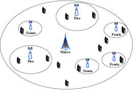
Figure 1: Illustration of heterogeneous cellular network composed of macro, pico and femtocell BSs and users.

II System Model

Fig. 1 shows a HCN consisting of three tiers of BSs (macro, pico and femtocell BSs) and mobile users. The scenario of multiple macro-cells is considered in our analysis although we only show a single macro-cell for the sake of simplicity. In this paper, we model downlink HCNs as $K$-tier BSs that are distinguished by their BS density $\lambda_{k}$, transmit power $P_{k}$, and SIR threshold $\beta_{k}$. The locations of BSs in each tier independently follow homogeneous PPP $\phi_{k}\,\left(1\leq k\leq K\right)$. The fading between BSs and any mobile user is assumed as temporally and spatially independent Rayleigh fading and the power fading coefficient between BS $x$ and the typical mobile user located at origin in time slot $t$ is denoted by $h_{x}(t)\sim exp(1).$ The standard singular path loss function is given as $g(x)=\frac{1}{\|x\|^{\alpha}},$ where $\alpha>2$ is the path loss exponent in $d$-dimensional plane. The analysis is conducted on a single frequency band. We assume that all BSs transmit packets continuously in all time slots at constant power. With the above notations, the interference of the typical user located at the origin and associated with BS $x_{i}$ in time slot $t$ is expressed as

$$I_{t}\left(x_{i}\right)=\sum_{l=1}^{K}\sum_{x\in\phi_{l},x\neq x_{i}}P_{l}h_{x}\left(t\right)g\left(x\right).$$ (1)

Since we assume noise is negligible, the received SIR of the user is accordingly given by

$$SIR_{t}\left(x_{i}\right)=\frac{P_{i}h_{x_{i}}\left(t\right)g\left(x_{i}\right)}{\sum_{l=1}^{K}\sum_{x\in\phi_{l},x\neq x_{i}}P_{l}h_{x}\left(t\right)g\left(x\right)}.$$ (2)

We consider an open access strategy [2], in which a mobile user can successfully associate with a BS in the $k^{th}$ tier only if its SIR with respect to that BS is greater than the corresponding threshold $\beta_{k}$. Under the assumption that $\beta_{k}>1,\>\forall k$, at most one BS in the entire network can provide SIR greater than the required threshold [2, Lemma 1].

III The Correlations of Interference in HCNs

Due to the stationarity of PPP, all users have the same interference distribution when the transmitters follow PPPs. Therefore, we may conduct analysis on a typical user located at the origin without loss of generality. However, interference is not independent across the plane or time slots. This is because interference is caused by the same random point processes [10]. In this section, we will investigate the spatio-temporal correlation of interference in HCNs and derive the correlation coefficient.

It has been previously observed that, when the standard singular path loss function $g(x)=\frac{1}{\|x\|^{\alpha}},\>\alpha>2$, is used, the average interference and its higher moments are infinite [16]. In this case, the correlation coefficient is undefined. Instead, we first use a bounded path loss function $g_{\varepsilon}\left(x\right)=\frac{1}{\|x\|^{\alpha}+\varepsilon},\>\varepsilon\in\left(0,\infty\right),\>\alpha>2$, to calculate the correlation coefficient and then consider the limiting case when $\varepsilon\downarrow 0$. The following Theorem gives the spatial and temporal correlation coefficient of interference in HCNs.

Theorem 1. The correlation coefficient of interference in HCNs where the BSs follow $K$-tier PPPs is

$$\rho\left(I_{t_{1}}(u),I_{t_{2}}(v)\right)=\frac{\int_{\mathbb{\mathbb{R}}^{d}}g(x)g(x-\|u-v\|)dx}{\mathbb{E}\left[h^{2}\right]\int_{\mathbb{\mathbb{R}}^{d}}g^{2}(x)dx}.$$ (3)

Further, the temporal correlation coefficient of interference ($\|u-v\|=0$) is expressed as

$$\rho_{t}=\frac{1}{\mathbb{E}\left[h^{2}\right]}.$$ (4)

The spatial correlation coefficient is given by

$$\underset{\varepsilon\downarrow 0}{\lim}\rho\left(I_{t}(u),I_{t}(v)\right)=0,\;u\neq v.$$ (5)

Proof:

See Appendix A. ∎

From Theorem 1, we can see that the correlation coefficient of interference is independent of the number of tiers, and the corresponding BS density and transmit power. To explain this unintuitive result, we consider a HCN without fading or mobility. In this case, the interference power received by a typical user remains the same for all time slots and the corresponding correlation coefficient is one. Different realizations of BSs, such as different number of tiers and the corresponding BS density and transmit power, will change the interference power at all time slots, without affecting the interference correlation. This is because they uniformly scale the interference. We also obtain that the correlation coefficient in HCNs is the same as that of ALOHA ad hoc networks (where the transmitters follow a PPP) with the ALOHA selection probability $p=1$. This is because the summation of several independent PPPs is still a PPP.

For $u=v$ and $t_{1}\neq t_{2}$, we obtain the temporal correlation coefficient which is only dependent on fading channels. If the channels are subject to independent Rayleigh fading with parameter 1, the temporal correlation coefficient is equal to 0.5. When $u\neq v$ and $t_{1}=t_{2}$, we obtain the spatial correlation coefficient for the standard singular path loss function when $\varepsilon\downarrow 0$. It should be noted that the spatial correlation coefficient being 0 is an artifact. The reason is as follows. When $g\left(x\right)=\frac{1}{\|x\|^{\alpha}}$, the interference created by user $u$ is mainly decided by the transmitters in a disc $B\left(u,r\right)$ centered at $u$ with a small radius $r>0$. In PPPs, the transmitters locations of different user in $B\left(u,r\right)$ and $B\left(v,r\right)$ are independent with each other for a small $r$. Therefore, the correlation coefficient goes to zero.

IV The Correlations of Link Successes in HCNs

In this section, joint success probabiltiy and conditional success probability are obtained to quantify the correlations of link successes in HCNs. The joint success probability is defined as the probability that a typical user accesses to a BS with SIR above its corresponding threshold in $n$ successive time slots. Under the assumption of SIR threshold $\beta_{k}>1\>for\,all\>k$, a user can connect to at most one BS among all BSs in the entire network at any given time slot. Furthermore, since no mobility is considered in this paper, a typical user always connects to the same BS in the $n$ time slots. According to the law of total probability, the joint success probability in HCNs is the summation of the probability that the user connects to every BS in HCNs. In other words, we have

$$p^{(n)}=\mathbb{E}_{\phi}\left[\sum_{i=1}^{K}\sum_{x_{i}\in\phi_{i}}p_{x_{i}}^{(n)}\right],$$ (6)

where $p_{x_{i}}^{(n)}$ denotes the probability that a typical user accesses to a given BS $x_{i}$ in $n$ successive time slots.

To derive $p^{(n)}$, we first calculate $p_{x_{i}}^{(n)}$. We also obtain some properties of the joint success probability. The conditional success probability is further derived based on the joint success probability.

IV-A Joint Success Probability of HCNs

Lemma 1. The probability that a typical user located at the origin accesses to the given BS $x_{i}$ in $n$ successive time slots is expressed as

$$p_{x_{i}}^{(n)}=P^{x_{i}}\left(A\left(t_{1}\right),A\left(t_{2}\right),\cdots,A\left(t_{n}\right)\right)$$

$$=\exp\left(-c_{d}\frac{\pi\delta}{\sin\pi\delta}\left(\frac{\beta_{i}}{P_{i}}\right)^{\delta}\sum_{l=1}^{K}\lambda_{l}P_{l}^{\delta}D_{n}\left(\delta\right)\cdot\|x_{i}\|^{d}\right),$$ (7)

where $A\left(t_{n}\right)$ represents the success event in $t_{n}$, $c_{d}$ is the volume of the $d$-dimensional unit ball, $\delta=\frac{d}{\alpha}$, and $D_{n}\left(\delta\right)$ denotes diversity polynomial [15] which is the multivariable polynomial given by $D_{n}\left(\delta\right)=\frac{\Gamma\left(n+\delta\right)}{\Gamma\left(n\right)\Gamma\left(1+\delta\right)}$ .

Proof:

See Appendix B. ∎

Lemma 1 gives a general expression for $d$-dimensional joint success probability of a user associated with the given BS $x_{i}$ in $n$ time slots. When $d=2$, the result is expressed as $\exp\left(-\pi\frac{\pi\delta}{\sin\pi\delta}\left(\frac{\beta_{i}}{P_{i}}\right)^{\delta}\sum_{l=1}^{K}\lambda_{l}P_{l}^{\delta}D_{n}\left(\delta\right)\cdot\|x_{i}\|^{2}\right)$. When $d=2$ and $K=1$, the result in Lemma 1 can be simplified to the special case of homogeneous ad hoc networks where the interferers follow a PPP. In this case, it is easy to see that we obtain the same result in [15] directly by setting $d=2,$ and $K=1$.

Under the assumption of $\beta_{i}>1,\>\forall i$, a user can access to at most one BS in the whole network. Therefore, the joint success probability in HCNs can be calculated by the sum of the probabilities that the user connects to each BS in $n$ time slots. This is because all the events are mutually exclusive and cannot happen at the same time. Note that the sum of probabilities over PPPs can be converted to a simple integral using Campbell-Mecke Theorem [17]. The expression of joint success probability in $n$ time slots is derived in the following Theorem.

Theorem 2. Given $\beta_{i}>1\>\forall i$, the joint success probability for a randomly located typical user in $n$ successive time slots is

$$p^{(n)} \overset{\triangle}{=} P\left(A\left(t_{1}\right),A\left(t_{2}\right),\cdots,A\left(t_{n}\right)\right)$$ (8)

$$= \frac{\sum_{i=1}^{K}\lambda_{i}P_{i}^{\delta}\beta_{i}^{-\delta}}{\frac{\pi\delta}{\sin\pi\delta}\cdot D_{n}\left(\delta\right)\cdot\sum_{l=1}^{K}\lambda_{l}P_{l}^{\delta}}.$$

Proof:

Due to the spatial stationarity of PPP, all the users have the same statistics of received signal [17]. Therefore, the analysis can be conducted on a typical user located at the origin. The joint success probability is:

$$p^{(n)} \overset{\triangle}{=}P\left(A\left(t_{1}\right),A\left(t_{2}\right),\cdots,A\left(t_{n}\right)\right)$$

$$\overset{\left(a\right)}{=} \mathbb{E}_{\phi}\left[\sum_{i=1}^{K}\sum_{x_{i}\in\phi_{i}}P^{x_{i}}\left(A\left(t_{1}\right),A\left(t_{2}\right),\cdots,A\left(t_{n}\right)\right)\right]$$

$$\overset{\left(b\right)}{=} \sum_{i=1}^{K}\mathbb{E}_{\phi}\left[\sum_{x_{i}\in\phi_{i}}P^{x_{i}}\left(A\left(t_{1}\right),A\left(t_{2}\right),\cdots,A\left(t_{n}\right)\right)\right]$$

$$\overset{\left(c\right)}{=} \sum_{i=1}^{K}\int_{\mathbb{R}^{d}}\lambda_{i}$$

$$\cdot \exp\left(-c_{d}\frac{\pi\delta}{\sin\pi\delta}\left(\frac{\beta_{i}}{P_{i}}\right)^{\delta}\sum_{l=1}^{K}\lambda_{l}P_{l}^{\delta}D_{n}\left(\delta\right)\|x_{i}\|^{d}\right)dx_{i}$$

$$= \sum_{i=1}^{K}c_{d}d\lambda_{i}\int_{0}^{\infty}$$

$$\exp\left(-c_{d}\frac{\pi\delta}{\sin\pi\delta}\left(\frac{\beta_{i}}{P_{i}}\right)^{\delta}\sum_{l=1}^{K}\lambda_{l}P_{l}^{\delta}D_{n}\left(\delta\right)r^{d}\right)r^{d-1}dr$$

$$= \frac{\sum_{i=1}^{K}\lambda_{i}P_{i}^{\delta}\beta_{i}^{-\delta}}{\frac{\pi\delta}{\sin\pi\delta}\cdot D_{n}\left(\delta\right)\cdot\sum_{l=1}^{K}\lambda_{l}P_{l}^{\delta}},$$

where $\left(a\right)$ comes from the assumption that $\beta_{i}>1\>\forall i$, $\left(b\right)$ follows from the linearity of the expectation, $\left(c\right)$ comes from the Campbell-Mecke Theorem. ∎

Although the result is not a closed-form expression, it is still a simple expression including the diversity polynomial $D_{n}\left(\delta\right)$ which can be calculated by using the gamma function. According to the properties of $D_{n}\left(\delta\right)$[15], the upper and lower bound of joint success probability in $n$ successive time slots is obtained in Corollary 1.

Corollary 1. The upper bound of the joint success probability is $\frac{1}{\frac{\pi\delta}{\sin\pi\delta}n^{\delta}}\cdot\frac{\sum_{i=1}^{K}\lambda_{i}P_{i}^{\delta}\beta_{i}^{-\delta}}{\sum_{l=1}^{K}\lambda_{l}P_{l}^{\delta}}$ and the lower bound is $\frac{\Gamma\left(1+\delta\right)}{\frac{\pi\delta}{\sin\pi\delta}n^{\delta}}\cdot\frac{\sum_{i=1}^{K}\lambda_{i}P_{i}^{\delta}\beta_{i}^{-\delta}}{\sum_{l=1}^{K}\lambda_{l}P_{l}^{\delta}}$.

Proof:

Note that $\alpha>d$, $\delta=\frac{d}{\alpha}$, so $0<\delta<1$. For all $\delta\in\left(0,1\right)$, $\frac{\Gamma\left(n+\delta\right)}{\Gamma\left(n\right)}\text{<}n^{\delta}$. From [15], we find that

$$n^{\delta}<D_{n}\left(\delta\right)<\frac{n^{\delta}}{\Gamma\left(1+\delta\right)}.$$ (9)

Substituting (9) into Theorem 1, we obtain the bounds of joint success probability. ∎

Next, we study the relationship between the joint success probability in $n$ time slots $p^{(n)}$ and the success probability in a single time slot $p^{(1)}$. Since $D_{1}\left(\delta\right)=1$, $p^{(1)}$ is expressed as

$$p^{(1)}=\frac{1}{\frac{\pi\delta}{\sin\pi\delta}}\cdot\frac{\sum_{i=1}^{K}\lambda_{i}P_{i}^{\delta}\beta_{i}^{-\delta}}{\sum_{l=1}^{K}\lambda_{l}P_{l}^{\delta}},$$ (10)

which coincides with the result in [2]. Comparing (8) and (10), the joint success probability can be expressed as $p^{(n)}=\frac{1}{D_{n}(\delta)}\cdot p^{(1)}.$ Therefore, $p^{(n)}$ is determined by both $p^{(1)}$ and the diversity polynomial $D_{n}(\delta)$ representing temporal correlation.

From the expression of $D_{n}(\delta)$, we see that the success event are fully correlated when $\delta\downarrow 0$ $\left(\alpha\uparrow\infty\right)$ and independent when $\delta\uparrow 1$ $\left(\alpha\downarrow 2\right)$. If $\delta\downarrow 0$ $\left(\alpha\uparrow\infty\right)$, $D_{n}\left(\delta\right)\downarrow 1$ for all $n$, so $p^{(1)}=p^{(2)}=\cdots=p^{(n)}$. In this case, the success events are fully correlated. The reason is that the interference is dominated by some near-by interferers. If they cause an outage at the current time slot, it is likely to do so at the next time slots. On the other hand, if $\delta\uparrow 1$ $\left(\alpha\downarrow 2\right)$, $D_{n}\left(\delta\right)\uparrow n$, the success events become independent. This is because the interference is influenced by many faraway interferers. The fading states between the interferers and the user in different time slots are independent, leading to independence in the corresponding interference. It is worth noting that at the same time, we have $p^{(n)}\downarrow 0$ since $\sin\left(\frac{2\pi}{\alpha}\right)\downarrow 0$ when $\alpha\downarrow 2$.

According to (8), the joint success probability in $n$ time slots is affected by BS density, SIR threshold, and transmit power. The following two corollaries tell us how the system parameters influence the joint success probability.

Corollary 2. Given the path loss exponent $\alpha$ and SIR threshold $\beta_{i}$, when the given SIR thresholds of various tiers are not all the same, the increase in BS density or transmit power improves the joint success probability under the condition that $\beta_{m}^{-\delta}>\frac{\sum_{i=1,i\neq m}^{K}\lambda_{i}P_{i}^{\delta}\beta_{i}^{-\delta}}{\sum_{i=1,i\neq m}^{K}\lambda_{i}P_{i}^{\delta}}$ . Otherwise, the increase in BS density or transmit power reduces the joint success probability.

Proof:

To prove the joint success probability $p^{(n)}$ increases with the BS density $\lambda_{m}$, we denote the constants $C_{0}=\frac{1}{\frac{\pi\delta}{\sin\pi\delta}D_{n}\left(\delta\right)}$, $C_{1}=\sum_{i=1,i\neq m}^{K}\lambda_{i}P_{i}^{\delta}\beta_{i}^{-\delta}$, $C_{2}=\lambda_{m}\beta_{m}^{-\delta}$, $D_{1}=\sum_{i=1,i\neq m}^{K}\lambda_{i}P_{i}^{\delta}$, $D_{2}=\lambda_{m}$. The joint success probability is expressed as

$$p^{(n)}=C_{0}\cdot\frac{C_{1}+C_{2}P_{m}^{\delta}}{D_{1}+D_{2}P_{m}^{\delta}}.$$ (11)

Taking the derivative with respect to $P_{m}$, we obtain

$$p^{\prime(n)}=C_{0}\cdot\frac{\delta\cdot P_{m}^{\delta-1}\left(C_{2}D_{1}-C_{1}D_{2}\right)}{\left[D_{1}+D_{2}\lambda_{m}\right]^{2}}.$$ (12)

Since $C_{0}>0$, $\delta>0$, and $P_{m}^{\delta-1}>0$, we have $p^{\prime(n)}>0$ when $C_{2}D_{1}>C_{1}D_{2}$. Thus, when $\beta_{m}^{-\delta}>\frac{\sum_{i=1,i\neq m}^{K}\lambda_{i}P_{i}^{\delta}\beta_{i}^{-\delta}}{\sum_{i=1,i\neq m}^{K}\lambda_{i}P_{i}^{\delta}}$, the joint success probability $p^{(n)}$ increases with the transmit power $P_{m}$ of the $m^{th}$ tier. On the other side, when $C_{2}D_{1}<C_{1}D_{2}$, we have $p^{\prime(n)}<0$. Therefore, the increase in transmit power $P_{m}$ of the $m^{th}$ tier will decrease the joint success probability under the condition that $\beta_{m}^{-\delta}<\frac{\sum_{i=1,i\neq m}^{K}\lambda_{i}P_{i}^{\delta}\beta_{i}^{-\delta}}{\sum_{i=1,i\neq m}^{K}\lambda_{i}P_{i}^{\delta}}$.

We can also show that the joint success probability increases with increasing BS density under the same condition, in a similar approach as the above, by denoting $C_{2}=P_{m}^{\delta}\beta_{m}^{-\delta}$ and $D_{2}=P_{m}^{\delta}$. This completes the proof. ∎

An intuitive explanation for Corollary 2 is the following. We know that increasing BS density or transmit power will increase the received power and the interference power at the same time. When the condition in Corollary 2 holds, the increase in the received power is greater than the increase in the interference power since the users have a high probability to access to the BSs in the $m^{th}$ tier. This is because the smaller the value of the SIR threshold of tier $m$ is, the higher probability the users will connect to the BSs in that tier, and the easier the above condition will hold at the same time. Therefore, the increase in transmit power and BS density of tier $m$ will result in the improvement of the joint success probability. Conversely, if the condition in Corollary 2 does not hold, the joint success probability is reduced by increasing the BS density or transmit power due to the inter-cell interference. We should note that Corollary 2 is obtained under the assumption that the given SIR thresholds of various tiers are not all the same. The next corollary tells us how the system parameters affect the joint success probability when all the tiers have the same SIR threshold.

Corollary 3. When all the tiers have the same SIR threshold ($\beta_{i}=\beta$), the joint success probability $p^{(n)}$ is expressed as

$$p^{(n)}=\frac{1}{\frac{\pi\delta}{\sin\pi\delta}D_{n}\left(\delta\right)\beta^{\delta}}.$$ (13)

which is only decided by the same SIR threshold $\beta$ and diversity polynomial $D_{n}\left(\delta\right)$ .

Proof:

We obtain (13) by substituting $\beta_{i}=\beta,\>\forall i$ into Theorem 1. ∎

When all tiers have the same SIR threshold, the users will choose the BSs depending only on the received SIR from that BS and the common SIR threshold. It means that the users cannot differentiate the BSs belonging to different tiers. Thus, the change to the number of tiers and their relative transmit power and BS density results in a change in interference power and signal power with the same factor. The corresponding effects are also canceled. Therefore, the joint success probability is only decided by SIR threshold $\beta$ and diversity polynomial $D_{n}\left(\delta\right)$ which represents temporal correlation. When there is a strong temporal correlation ($\alpha\uparrow\infty$), the joint success probability is high. Otherwise, the joint success probability is low. Especially, when $\alpha\downarrow 2$, the joint success probability approximates to 0.

Next, the conditional success probability given $n-1$ successes is obtained as another metric to quantify the correlations of link successes.

IV-B The Conditional Success Probability

In this section, we investigate the conditional success probability which is defined as the probability that the $n$ attempt succeeds when the first $n-1$ ones did. Note that it is another metric to quantify the correlations of link successes.

Corollary 4. The conditional success probability given n successes in HCNs is expressed as

$$P\left(A_{t_{n}}|A_{t_{1}},A_{t_{2}},\cdots,A_{t_{n-1}}\right)$$

$$= \frac{P\left(A_{t_{1}},A_{t_{2}},\cdots,A_{t_{n}}\right)}{P\left(A_{t_{1}},A_{t_{2}},\cdots,A_{t_{n-1}}\right)}$$ (14)

$$= \frac{D_{n-1}\left(\delta\right)}{D_{n}\left(\delta\right)},$$

which is decided only by the number of time slots n and path loss exponent $\alpha$ ($\delta$ is determined by $\alpha$ and $\delta=\frac{d}{\alpha}$).

Proof:

We obtain this result directly by substituting (8) into (14). ∎

From Corollary 4, we see that the conditional success probability is independent of BS density, transmit power, and SIR threshold and it only depends on the path loss exponent $\alpha$ and the number of time slots $n$. For $n\uparrow\infty$, we get that $P\left(A_{t_{n}}|A_{t_{1}},A_{t_{2}},\cdots,A_{t_{n-1}}\right)\uparrow 1$. It shows that the $n$ attempt will succeed with probability 1 when the first $n-1$ ones succeed.

IV-C Comparison with the Special Cases in the Existing Work

In this section, we will derive the joint success probability of some special cases that have been studied in existing works, by setting specific system parameters in the above analysis. Further, the relationship between them and our result is obtained.

IV-C1 SIMO System

When $K=1$, the system in our paper can be simplified to a SIMO system where the interferers come from a stationary Poisson point process and the receiver under consideration is equipped with $n\geq 1$ antennas [15]. In this case, the SIR in different time slots in our paper should be considered as the SIR at different antennas in [15]. It is worth noting that in [15], the authors assume that the desired transmitter is added at a distance $r$ from the receiver, which is different from our system. Therefore, there is no cell association in [15]. We obtain the probability that the SIR at all antennas exceeds SIR threshold $\beta$ [15, Theorem 1] by setting $d=2$, $c_{d}=\pi$, $P=1$, $\parallel x_{i}\parallel=r$ in Lemma 1 since we do not consider cell association in Lemma 1. The corresponding probability is expressed as $\exp\left(-\frac{\pi^{2}\delta}{\sin\left(\pi\delta\right)}\cdot\lambda\cdot r^{2}\cdot\beta^{\delta}\cdot D_{n}\left(\delta\right)\right)$. Based on the property of the gamma function $\Gamma\left(1-\delta\right)\Gamma\left(1+\delta\right)=\frac{\pi\delta}{\sin\left(\pi\delta\right)}$, the above probability is the same as the result in [15, Theorem 1]. Note that the diversity polynomial $D_{n}\left(\delta\right)$ quantifies the spatial diversity in [15] instead of the temporal diversity in our paper.

IV-C2 Ad hoc Networks

When $K=1$, our system model can also be seemed as an ad hoc network where the transmitters follow a stationary PPP. In particular, this special case is the same as the ALOHA ad hoc network investigated in [10] with transmission probability $p=1$. In [10], the distance between the transmitter and its receiver is assumed as a constant, which is different to our model. We can obtain the joint success probability in [10] by setting $d=2$, $c_{d}=\pi$, $P=1$, $\parallel x_{i}\parallel=r$ and $n=2$ in Lemma 1. This is because the cell association is not cosindered in Lemma 1. It is worth noting that the authors in [10] did not derive the closed-form expression.

IV-C3 HCNs without considering temporal correlations

If we only consider a single time slot ($n=1$), there is no interference correlation. Correspondingly, the diversity polynomial $D_{n}\left(\delta\right)$ equals to one. Therefore, the success probability of HCNs in one time slot is expressed as $p^{(1)}=\frac{1}{\frac{\pi\delta}{\sin\pi\delta}}\cdot\frac{\sum_{i=1}^{K}\lambda_{i}P_{i}^{\delta}\beta_{i}^{-\delta}}{\sum_{l=1}^{K}\lambda_{l}P_{l}^{\delta}}$ which coincides with the result in [2, Corollary 1] with no noise. Further, if $K=1$ or all the tiers have the same SIR threshold $\beta_{i}=\beta,\>\forall i$, the success probability in a single time slot is simplified to $p^{(1)}=\frac{1}{\frac{\pi\delta}{\sin\pi\delta}}\cdot\beta^{-\delta}$, which is only decided by the SIR threshold and the path loss exponent.

IV-D Special Case of Interest

To avoid cross-tier interference, one option is to allocate separated spectrum to the BSs in different tiers. In this special case, the interference received by a typical user comes from the BSs in the same tier and is expressed as $I_{t}\left(x_{i}\right)=\sum_{x\in\phi_{i},x\neq x_{i}}P_{i}h_{x}\left(t\right)g\left(x\right)$. According to the result in Lemma 1, the probability that a typical user connects to the given BS $x_{i}$ in $n$ successive time slots is given by

$$p_{x_{i}}^{(n)}=\exp\left(-c_{d}\frac{\pi\delta}{\sin\pi\delta}\lambda_{i}\beta_{i}^{\delta}D_{n}\left(\delta\right)\cdot\|x_{i}\|^{d}\right).$$ (15)

It is worth noting that if we consider the two-dimensional space, the above expression is the same as the result of Theorem 1. in [11]. This is because the interference only comes from a PPP, and fixed distance between transmitter and receiver is considered.

Next, based on the assumption of $\beta_{i}>1,\>\forall i$, and the Campbell-Mecke Theorem, we obtain the joint success probability that the typical user accesses to the BSs in tier $i$ as

$$p_{i}^{(n)}=\frac{\beta_{i}^{-\delta}}{\frac{\pi\delta}{\sin\pi\delta}D_{n}\left(\delta\right)}.$$ (16)

The joint success probability of a typical tier is only dependent on the SIR threshold of the corresponding tier and the path loss exponent.

V Numerical Results

In this section, using Matlab and Monte Carlo methods, we first validate the correlation coefficient and joint success probability in Theorem 1 and Theorem 2, respectively. Then, the effect of SIR threshold, BS density, and transmit power on the joint success probability is discussed.

In the simulations, the locations of BSs in each tier follow a PPP. The typical user is assumed at the origin. The fading channels are generated as independent Rayleigh random variables. The user chooses the strongest BS in terms of the received SIR and the SIR is evaluated by (2). In each Monte Carlo trial, the channel gains and the locations of BSs are generated independently.

Fig. 2 shows the correlation coefficient of interference varying with $\|u-v\|$ for $\alpha=4$, $\mathbb{E}\left[h^{2}\right]=2$, and $g_{\varepsilon}\left(x\right)=\frac{1}{\|x\|^{\alpha}+\varepsilon},\>\varepsilon$ taking small positive values. We observe that the correlation coefficient of interference reaches the maximum value when $\|u-v\|=0$. This gives the temporal correlation coefficient at the same location. Note that it is only dependent on $\mathbb{E}\left[h^{2}\right]$ since $\rho_{t}=\frac{1}{\mathbb{E}\left[h^{2}\right]}$. The correlation coefficient decreases with the increase of $\|u-v\|$, which coincides with our intuition. The farther the distance is, the smaller the correlation coefficient is. When $\varepsilon\downarrow 0$, the correlation coefficient goes to zero. This is because the interference is dominated by the transmitters located near to the receiver and the interferers for different receivers are independent in PPPs.

Fig. 3 shows the joint success probability of two-tier HCNs represented by simulated results, analytical results, the corresponding upper and lower bound, and the independent case. From Fig. 3, we first notice that an analysis that ignores the interference correlation (i.e., the independent case) can substantially under estimate the joint success probability. We further observe that the simulated results coincide with the analytical results very well even for $\beta_{2}=-4dB$. The upper and lower bounds are also close to the analytical results. Further, we observe that the joint success probability decreases with the increase of SIR threshold. This is because it is harder for the users to obtain satisfactory SIR when the SIR threshold increases.

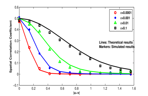
Figure 2: Correlation coefficient of interference versus $\|u-v\|$

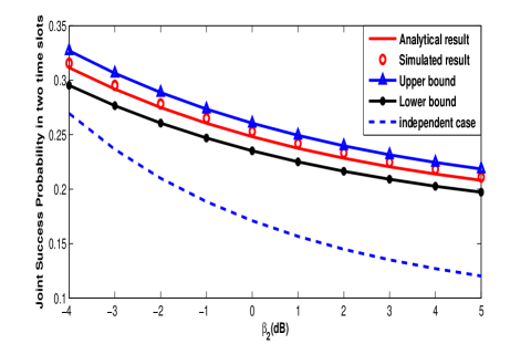
Figure 3: Joint success probability in a two-tier HCNs ($n=2$, $K=2$, $P_{1}=10P_{2}$, $\lambda_{2}=2\lambda_{1}$, $\beta_{1}=0dB$, $\alpha=3$).

Fig. 4 and Fig. 5 show the influence of BS density and transmit power of the second tier on the joint success probability. When $K=2$, the condition in Corollary 2 is simplified to $\beta_{2}<\beta_{1}$. When $\beta_{2}=-4dB$ and $\beta_{2}=-2dB$, the above condition holds ($\beta_{2}<\beta_{1}$). Hence, the joint success probability is improved by increasing the BS density and transmit power of tier two. The reason is that the users prefer to access to the BSs in the second tier when the condition holds. Thus, increasing the BS density or transmit power leads to a higher increase in the received power than that in the interference. When the condition in Corollary 2 does not hold, the joint success probability decreases with increasing the BS density or transmit power, since the resulting increase in the received power is less than that in the interference. When $\beta_{2}=1dB$ ($\beta_{1}=\beta_{2}$), the joint success probability does not vary with the change of BS density or transmit power. This is because the change in the above system parameters results in the same change in the received power and the interference and thus the effect can be canceled.

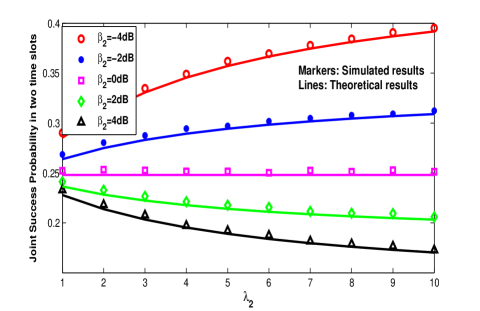
Figure 4: Joint success probability in a two-tier HCNs ($n=2,$ $K=2$, $P_{1}=10P_{2}$, $\lambda_{1}=1$, $\beta_{1}=0dB$, $\alpha=3$)

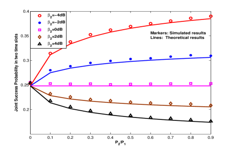
Figure 5: Joint success probability in a two-tier HCNs ($n=2,$ $K=2$, $P_{1}=100$, $\lambda_{2}=2\lambda_{1}$, $\beta_{1}=0dB$, $\alpha=3$)

In Fig. 6, we present the conditional success probability in a two-tier HCNs varying with the number of time slots. From this figure, we see that the conditional success probability is dramatically enhanced in the first and second slots. Further, the conditional success probability approximates to 1 when $n\rightarrow\infty$. At the same time slot, the greater the path loss exponent is, the higher the conditional success probability is, which coincides with our intuition. The interference is mainly determined by some nearest interferers when there is a large path loss exponent. Therefore, the successes in the previous time slots will lead to success in the current time slot with a high probability.

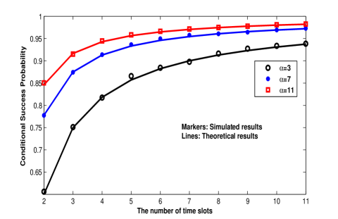
Figure 6: Conditional success probability in a two-tier HCNs ($n=2,$ $K=2$, $P_{1}=10P_{2}$, $\lambda_{2}=2\lambda_{1}$, $\beta_{1}=0dB$)

VI Conclusions

In this paper, we investigated the correlations of interference and link successes which are quantified by the correlation coefficient and joint success probability in HCNs. Based on the $K$-tier Poisson network model, Rayleigh fading, and SIR threshold greater than one, we derived the expressions of the above metrics. From our analytical results, we revealed how the system parameters affect the interference correlation and the joint success probability. We showed that the interference correlation coefficient is independent of the number of tiers, BS density, and transmit power. Further, we observed that the temporal correlation coefficient is dependent only on channel fading. However, although the parameters of HCNs do not change the correlations of interference, they have an important influence on the correlations of link outages. When the SIR thresholds are not all the same, joint success probability is enhanced with the increase in BS density or transmit power under a certain condition. When all tiers have the same SIR threshold, the joint success probability is only decided by the diversity polynomial and the SIR threshold. Finally, we obtained the conditional success probability after $n-1$ successes, which is another metric to quantify the correlations of link successes. We observed that the conditional success probability is only dependent on the number of time slots and path loss exponent.

Appendix A Appendix: Proofs

A-A Proof of Theorem 1

Proof:

According to our system model, the interference of a randomly selected user located at $u$ at time slot $t$ is expressed as $I_{t}\left(u\right)=\sum_{l=1}^{K}\sum_{x\in\phi_{l},x\neq x_{i}}P_{l}h_{x}\left(t\right)g\left(x-u\right).$ Since all users have the same interference distribution, we can conduct the analysis on a typical user located at the origin. The average interference is given by

$$\mathbb{E}\left[I_{t}\left(u\right)\right] =\mathbb{E}\left[I_{t}\left(o\right)\right]$$

$$=\mathbb{E}\left[\sum_{j=1}^{K}\sum_{x\in\phi_{j},x\neq x_{u}}P_{j}h_{x}\left(t\right)g\left(x\right)\right]$$

$$\overset{\left(a\right)}{=}\sum_{j=1}^{K}\mathbb{E}_{\phi_{j}}\left[\sum_{x\in\phi_{j},x\neq x_{u}}\mathbb{E}_{h}\left[P_{j}h_{x}\left(t\right)g\left(x\right)\right]\right]$$

$$\overset{\left(b\right)}{=}\sum_{j=1}^{K}\lambda_{j}\int_{\mathbb{\mathbb{R}}^{d}}\mathbb{E}[h]P_{j}g(x)dx$$

$$=\sum_{j=1}^{K}\lambda_{j}P_{j}\int_{\mathbb{\mathbb{R}}^{d}}g(x)dx,$$ (17)

where $\left(a\right)$ comes from the linearity of the expectation, $\left(b\right)$ follows from Campbell-Mecke Theorem.

The mean product of $I_{t_{1}}(u)$ and $I_{t_{2}}(v)$ at different time slots $t_{1}$and $t_{2}$ is given by

$$\mathbb{E}[I_{t_{1}}(u),I_{t_{2}}(v)]$$

$$=\mathbb{E}[\sum_{j=1}^{K}\sum_{\underset{x\neq x_{u}}{x\in\phi_{j}}}P_{j}h_{x}(t_{1})g(x-u)\sum_{q=1}^{K}\sum_{\underset{x\neq y_{v}}{y\in\phi_{q}}}P_{q}h_{y}(t_{2})g(y-v)]$$

$$=\mathbb{E}[\sum_{j=1}^{K}\sum_{\underset{x\neq x_{u}}{x\in\phi_{j}}}P_{j}h_{x}(t_{1})g(x-u)\cdot P_{j}h_{x}(t_{2})g(x-v)$$

$$+\sum_{j=1}^{K}\sum_{\underset{x\neq x_{u},x\neq y}{x\in\phi_{j}}}\sum_{q=1}^{K}\sum_{\underset{x\neq y_{v},x\neq y}{y\in\phi_{q}}}P_{j}h_{x}(t_{1})g(x-u)\cdot P_{q}h_{y}(t_{2})g(y-v)]$$

$$\overset{\left(a\right)}{=}\sum_{j=1}^{K}P_{j}^{2}(\mathbb{E}[h])^{2}\lambda_{j}\int_{\mathbb{\mathbb{R}}^{d}}g(x-u)g(x-v)dx$$

$$+\sum_{j=1}^{K}\sum_{q=1}^{K}P_{j}P_{q}(\mathbb{E}[h])^{2}\lambda_{j}\lambda_{q}\int_{\mathbb{\mathbb{R}}^{d}}g(x-u)dx\int_{\mathbb{\mathbb{R}}^{d}}g(y-v)dy$$

$$=\sum_{j=1}^{K}P_{j}^{2}\lambda_{j}\int_{\mathbb{\mathbb{R}}^{d}}g(x-u)g(x-v)dx$$

$$+\sum_{j=1}^{K}\sum_{q=1}^{K}P_{j}P_{q}\lambda_{j}\lambda_{q}(\int_{\mathbb{\mathbb{R}}^{d}}g(x)dx)^{2},$$ (18)

where $\left(a\right)$follows by the second order product density of PPPs and Campbell’s theorem.

The second moment of the interference is expressed as

$$\mathbb{E}\left[I_{t}^{2}(u)\right] =\mathbb{E}\left[I_{t}^{2}(o)\right]$$

$$=\mathbb{E}\left[\left(\sum_{j=1}^{K}\sum_{x\in\phi_{j},x\neq x_{u}}P_{j}h_{x}(t)g(x)\right)^{2}\right]$$

$$=\mathbb{E}\left[\sum_{j=1}^{K}\sum_{x\in\phi_{j},x\neq x_{u}}P_{j}^{2}h_{x}^{2}(t)g^{2}(x)\right]$$

$$+\mathbb{E}\left[\sum_{j=1}^{K}\sum_{\underset{x\neq x_{u},x\neq y}{x\in\phi_{j}}}\sum_{q=1}^{K}\sum_{\underset{x\neq y_{v},x\neq y}{y\in\phi_{q}}}P_{j}h_{x}(t)g(x)\cdot P_{q}h_{y}(t)g(y)\right]$$

$$=\sum_{j=1}^{K}P_{j}^{2}\mathbb{E}\left[h^{2}\right]\lambda_{j}\int_{\mathbb{\mathbb{R}}^{d}}g^{2}(x)dx$$

$$+\sum_{j=1}^{K}\sum_{q=1}^{K}P_{j}P_{q}(\mathbb{E}[h])^{2}\lambda_{j}\lambda_{q}(\int_{\mathbb{\mathbb{R}}^{d}}g(x)dx)^{2}.$$ (19)

The variance of the interference is given by

$$VAR\left[I_{t}(u)\right] =\mathbb{E}[I_{t}^{2}(u)]-\left(\mathbb{E}[I_{t}(u)]\right)^{2}$$

$$=\sum_{j=1}^{K}P_{j}^{2}\mathbb{E}\left[h^{2}\right]\lambda_{j}\int_{\mathbb{\mathbb{R}}^{d}}g^{2}(x)dx.$$ (20)

The correlation coefficient of two random variables is expressed as

$$\rho\left(X_{1},X_{2}\right) =\frac{cov\left(X_{1},X_{2}\right)}{\sqrt{var\left(X_{1}\right)}\cdot\sqrt{var\left(X_{1}\right)}}$$

$$=\frac{\mathbb{E}\left[X_{1},X_{2}\right]-\mathbb{E}\left[X_{1}\right]\mathbb{E}\left[X_{2}\right]}{\sqrt{var\left(X_{1}\right)}\cdot\sqrt{var\left(X_{1}\right)}}.$$ (21)

Substituting (18), (17), and (20) into (21), we obtain the spatial-temporal correlation coefficient of the interference $I_{t_{1}}(u)$ and $I_{t_{2}}(v)$ that

$$\rho\left(I_{t_{1}}(u),I_{t_{2}}(v)\right) =\frac{\int_{\mathbb{\mathbb{R}}^{d}}g(x)g(x-\|u-v\|)dx}{\mathbb{E}\left[h^{2}\right]\int_{\mathbb{\mathbb{R}}^{d}}g^{2}(x)dx}.$$ (22)

The temporal correlation coefficient is obtained as $\rho_{t}=\frac{1}{\mathbb{E}\left[h^{2}\right]}$ by setting $\|u-v\|=0$. Note that the above derivation is obtained when $g\left(x\right)$ is defined as a bounded path loss function $g_{\varepsilon}\left(x\right)=\frac{1}{\|x\|^{\alpha}+\varepsilon},\>\varepsilon\in\left(0,\infty\right),\>\alpha>d$. However, we obtain the correlation coefficient for the singular path loss as $\varepsilon\downarrow 0$. The spatial correlation coefficient is given by $\underset{\varepsilon\downarrow 0}{\lim}\rho\left(u,v\right)=0,\;u\neq v$ [10]. ∎

A-B Proof of Lemma 1

Proof:

Recall that the fading is averaged out, a user connects to the strongest BS in terms of the long-term averaged received power. Since no mobility is considered in our paper, the user is associated with the same BS in $n$ successive time slots. Given BS $x_{i}$, the joint success probability of a typical user located at the origin is:

$$p_{x_{i}}^{(n)}= P^{x_{i}}\left(A\left(t_{1}\right),A\left(t_{2}\right),\cdots,A\left(t_{n}\right)\right)$$

$$= \mathbb{P}\left(SIR_{t_{1}}(x_{i})>\beta_{i},SIR_{t_{2}}(x_{i})>\beta_{i},\cdots,SIR_{t_{n}}(x_{i})>\beta_{i}\right)$$

$$= \mathbb{P}\left(\frac{P_{i}h_{x_{i}}(t_{1})g(x_{i})}{I_{t_{1}}(x_{i})}>\beta_{i},\cdots,\frac{P_{i}h_{x_{i}}(t_{n})g(x_{i})}{I_{t_{n}}(x_{i})}>\beta_{i}\right)$$

$$= \mathbb{P}\left(h_{x_{i}}(t_{1})>\frac{\beta_{i}I_{t_{1}}(x_{i})}{P_{i}g(x_{i})},\cdots,h_{x_{i}}(t_{n})>\frac{\beta_{i}I_{t_{n}}(x_{i})}{P_{i}g(x_{i})}\right)$$

$$\overset{\left(a\right)}{=} \mathbb{E}_{I_{t}}\left[\exp\left(-\frac{\beta_{i}\left(I_{t_{1}}(x_{i})+I_{t_{2}}(x_{i})+\cdots I_{t_{n}}(x_{i})\right)}{P_{i}g(x_{i})}\right)\right]$$

$$\overset{\left(b\right)}{=} \mathbb{E}_{I_{t}}\left[\exp\left(-\frac{\beta_{i}P_{l}g(x)}{P_{i}g(x_{i})}\sum_{l=1}^{K}\sum_{,\underset{x\neq x_{i}}{x\in\phi_{l}}}\left(h_{x}(t_{1})+\cdots+h_{x}\left(t_{n}\right)\right)\right)\right]$$

$$=\Pi_{l=1}^{K} \mathbb{E}_{\phi_{l}}\left[\underset{\underset{x\neq x_{i}}{x\in\phi_{l}}}{\Pi}\mathbb{E}_{h}\left[\exp\left(-\frac{\beta_{i}P_{l}g(x)}{P_{i}g(x_{i})}\left(h_{x}(t_{1})+\cdots+h_{x}\left(t_{n}\right)\right)\right)\right]\right]$$

$$\overset{\left(c\right)}{=} \Pi_{l=1}^{K}\mathbb{E}_{\phi_{l}}\left[\underset{\underset{x\neq x_{i}}{x\in\phi_{l}}}{\Pi}\left(\frac{1}{1+\frac{\beta_{i}P_{l}g(x)}{P_{i}g(x_{i})}}\right)^{n}\right]$$

$$\overset{\left(d\right)}{=} \Pi_{l=1}^{K}\exp\left(-\lambda_{l}\int_{\mathbb{R}^{d}}\left[1-\left(\frac{1}{1+\frac{\beta_{i}P_{l}g(x)}{P_{i}g(x_{i})}}\right)^{n}\right]dx\right)$$

$$\overset{\left(e\right)}{=} \exp\left(-c_{d}\frac{\pi\delta}{\sin\pi\delta}\left(\frac{\beta_{i}}{P_{i}}\right)^{\delta}\sum_{l=1}^{K}\lambda_{l}P_{l}^{\delta}D_{n}\left(\delta\right)\cdot\|x_{i}\|^{d}\right),$$

where $\left(a\right)$ comes from the independence of $h_{x_{i}}(t_{1})$ , $h_{x_{i}}(t_{2})$,$\cdots$, $h_{x_{i}}(t_{n})$ , $\left(b\right)$ follows from the expression of interference $I_{t}\left(x_{i}\right)=\sum_{l=1}^{K}\sum_{x\in\phi_{l},x\neq x_{i}}P_{l}h_{x}\left(t\right)g\left(x\right)$, $\left(c\right)$ follows by taking the average with respect to $h_{x}(t_{1})$ , $h_{x}(t_{2})$,$\cdots$, $h_{x}(t_{n})$, $\left(d\right)$ comes from probability generating functional of PPP, and $\left(e\right)$ follows from the calculation of the integral [15]. ∎

References

- [1] K. Mallinson, “The 2020 vision for LTE,” http://www.fiercewireless.com/europe/story/mallinson-2020-vision-lte/2012-06-20, Tech. Rep.
- [2] H.S.Dhillon, R.K.Ganti, F.Baccelli, and J.G.Andrews, “Modeling and analysis of k-tier downlink heterogeneous cellular networks,” IEEE J. Sel. Areas Commun., vol. 30, no. 3, pp. 550–560, April 2012.
- [3] H.-S. Jo, Y. J. Sang, P. Xia, and J. Andrews, “Heterogeneous cellular networks with flexible cell association: A comprehensive downlink sinr analysis,” IEEE Trans. Wireless Commun., vol. 11, no. 10, pp. 3484–3495, 2012.
- [4] H. Dhillon, R. Ganti, and J. Andrews, “Load-aware modeling and analysis of heterogeneous cellular networks,” IEEE Trans. Wireless Commun., vol. 12, no. 4, pp. 1666–1677, 2013.
- [5] S. Mukherjee, “Distribution of downlink sinr in heterogeneous cellular networks,” IEEE J. Sel. Areas Commun., vol. 30, no. 3, pp. 575–585, April 2012.
- [6] W. Bao and B. Liang, “Structured spectrum allocation and user association in heterogeneous cellular networks,” in Proc. IEEE INFOCOM, 2014, pp. 1069–1077.
- [7] S. Singh, H. Dhillon, and J. Andrews, “Offloading in heterogeneous networks: Modeling, analysis, and design insights,” IEEE Trans. Wireless Commun., vol. 12, no. 5, pp. 2484–2497, 2013.
- [8] J. Wen, M. Sheng, X. Wang, J. Li, and H. Sun, “On the capacity of downlink multi-hop heterogeneous cellular networks,” IEEE Trans. Wireless Commun., vol. 13, no. 8, pp. 4092–4103, Aug 2014.
- [9] U. Schilcher, C. Bettstetter, and G. Brandner, “Temporal correlation of interference in wireless networks with rayleigh block fading,” IEEE Trans. Mobile Comp., vol. 11, no. 12, pp. 2109–2120, Dec 2012.
- [10] R. Ganti and M. Haenggi, “Spatial and temporal correlation of the interference in aloha ad hoc networks,” IEEE Commun. Lett., vol. 13, no. 9, pp. 631–633, Sept 2009.
- [11] M. Haenggi and R. Smarandache, “Diversity polynomials for the analysis of temporal correlations in wireless networks,” IEEE Trans. Wireless Commun., vol. 12, no. 11, pp. 5940–5951, November 2013.
- [12] Z. Gong and M. Haenggi, “Interference and outage in mobile random networks: Expectation, distribution, and correlation,” IEEE Trans. Mobile Comp., vol. 13, no. 2, pp. 337–349, 2014.
- [13] R. Tanbourgi, H. S. Dhillon, J. G. Andrews, and F. K. Jondral, “Effect of spatial interference correlation on the performance of maximum ratio combining,” IEEE Trans. Wireless Commun., July, 2013.
- [14] Y. Zhong, W. Zhang, and M. Haenggi, “Managing interference correlation through random medium access,” IEEE Trans. Wireless Commun., vol. PP, no. 99, pp. 1–14, 2014.
- [15] M.Haenggi, “Diversity loss due to interference correlation,” IEEE Commun. Lett., vol. 16, no. 10, pp. 1600–1603, October 2012.
- [16] M. Haenggi and R. Ganti, Interference in large wireless netwoks. Now Publishers Inc, 2009.
- [17] F. Baccelli and B. Blaszczyszyn, Stochastic Geometry and Wireless Networks, Volume 1: Theory. NOW, Dec. 2009.