Large-deviation properties of resilience of power grids

Abstract

We study the distributions of the resilience of power flow models against transmission line failures via a so-called backup capacity. We consider three ensembles of random networks and in addition, the topology of the British transmission power grid. The three ensembles are Erdős-Rényi random graphs, Erdős-Rényi random graphs with a fixed number of links, and spatial networks where the nodes are embedded in a two dimensional plane. We investigate numerically the probability density functions (pdfs) down to the tails to gain insight in very resilient and very vulnerable networks. This is achieved via large-deviation techniques which allow us to study very rare values which occur with probability densities below $10^{-160}$. We find that the right tail of the pdfs towards larger backup capacities follows an exponential with a strong curvature. This is confirmed by the rate function which approaches a limiting curve for increasing network sizes. Very resilient networks are basically characterized by a small diameter and a large power sign ratio. In addition, networks can be made typically more resilient by adding more links.

1 Introduction

Stability and control of power grids have not only been investigated by engineers [1, 2], where rotor angle and voltage stability play an important role, but attracted also attention in the physics community. By generalizing the swing equation [1, 2] of a synchronous machine to small networks by using the well studied Kuramoto model [3, 4], Filatrella, Nielsen and Pedersen [5] stimulated many studies in this field. In [6] the synchronization of this dynamical model on the topology of the power grid of the United Kingdom (UK) is investigated. While [7, 8] analyzed this Kuramoto-like model with respect to its application for power grids, in [9, 10] synchrony optimized networks with Kuramoto oscillators were constructed. More generally, synchronization of oscillators with spectral methods was put under scrutiny in [11, 12, 13].

In addition, many studies [14, 15, 16, 17, 18, 19, 20, 21, 22] deal with load models and analyze the vulnerability of networks due to node failures and the resulting cascading failures that might occur.

Here, we are not interested in the stability of dynamical systems but the resilience of networks. In [23] the resilience of a very basic model for transportation networks was investigated via introducing a “backup capacity” (see below) and using large-deviation techniques. The model in [23] assumes that one unit of some “quantity” is transported between all pairs of nodes along shortest paths. In the present work, we study a very different model, still quite simple but designed for modelling power grids, based on the laws of electricity. Specifically, we introduce a power flow model on networks based on the fixed points of a Kuramoto-like model [5, 6] and a linearized DC power flow model (see e.g., [24]) as used in electrical engineering, respectively.

The resilience is defined by the backup capacity. This quantity measures the overcapacity of the transmission lines which is needed to ensure stable operation when the most loaded link in the network exhibits a failure. We obtain the probability density functions (pdfs) of the resilience for three different random network ensembles and the topology of the power grid of the UK.

We are interested in obtaining the pdfs of these ensembles over a large range of the support, because a probability distribution contains the full information of a stochastic system in contrast to a finite number of moments (like e.g., mean or variance). To make statements about the different ensembles concerning the resilience we therefore need the whole pdf including the low-probability tails. By obtaining these tails we are also able to get properties of very vulnerable (high backup capacity) and very resilient (low backup capacity) networks. The analysis of these very resilient networks allows us to derive design principles for a resilient future power grid.

Furthermore, given the backup capacity of an existing network, one can compare with a suitable network ensemble. The cumulative probability of finding a more resilient network (with smaller backup capacity) in the ensemble yields a quality measure for the investigated network. This is the so-called $p$-value, which is a standard quantity in statistics to estimate the significance of a result. Sometimes, one needs to access the low probability tails of a pdf like in the present approach, where we want to study optimized high-resilience power grids. This is analogous to the calculation of significance of protein alignments, where one also needs to access the tails of the pdf, since proteins are optimized by evolution [25]. For an example of the $p$-value calculation, see section 6.1.

The paper is organized as follows. In section 2 the studied model and its simplification to static flow equations is described. Section 3 deals with the determination of the backup capacity and hence the resilience of a network against transmission line failures. Next, section 4 presents the investigated random network ensembles as well as the topology of an existing power grid. After this, the simulation and reweighting techniques are explained in section 5, followed by section 6 which provides the numerical results of the simulations. Last, a conclusion is drawn and a short outlook is given.

2 Model

2.1 Kuramoto-like model

We use a simplified model of interconnected synchronous machines, derived from the dynamics of the rotor to model a power grid. The classic constant-voltage behind the transient-reactance model then gives the swing equations (see e.g., [1, 8]) which are derived from energy conservation. The Kuramoto-like model used in [5, 6, 8] is directly related to this swing equation. On each node $i$ of the network either a synchronous generator or a synchronous motor are placed. The generators exhibit power plants and therefore produce power ($P_{i}^{\rm source}>0$), whereas the motors consume power ($P_{i}^{\rm source}<0$).

Note that only active power is considered here and all transmission lines are regarded as lossless. These simplification appear justified to us, since for the first time the resilience properties of models for electric power grids are studied over the almost complete ensemble, even in the regime of extreme networks. Thus, our work lays a solid ground for later comparisons to more sophisticated models. E.g., in [8, 1] an extension of the model studied here to transmission lines with losses (using the admittance matrix) as well as nodal voltages is explained. A further expansion of the model with reactive power is given in [7].

Each synchronous machine $i$ can be described [5, 6] by its mechanical phase $\theta_{i}=\Omega t+\phi_{i}$, where $\Omega$ is the angular frequency ($2\pi\cdot 50$ or $2\pi\cdot 60$ rad s^-1) and $\phi_{i}$ the phase deviation. Note that the mechanical phase deviation $\phi_{i}$ is the same as the electrical angle $\delta_{\rme}$ except for a constant factor, namely the number of poles $n_{\rm{P}}$ of the synchronous machine [1]: $\delta_{\rme}=(n_{\rm{P}}/2)\phi_{i}$. To derive the equation of motion for $\phi_{i}$, one needs to consider energy (or power) conservation [5, 6], so that for each synchronous machine $i$

$$P_{i}^{\rm source}=P_{i}^{\rm diss}+P_{i}^{\rm acc}+P_{i}^{\rm flow},$$ (1)

where $P_{i}^{\rm{source}}\gtrless 0$ depending on whether the machine is a generator or a motor. $P_{i}^{\rm diss}$ and $P_{i}^{\rm acc}$ are the dissipated and accumulated power, respectively. The power flow between two units $i$ and $j$ is given by [5, 6]

$$P_{ij}^{\rm flow}=-P_{ij}^{\rm MAX}\sin(\theta_{j}-\theta_{i}),$$ (2)

where $P_{ij}^{\rm MAX}$ is the maximum capacity of the power line, which connects the nodes $i$ and $j$. The power flow of node $i$ is therefore given by the sum of the flow to all its neighbors

$$P_{i}^{\rm flow}=-\sum_{j}P_{ji}^{\rm MAX}\sin(\phi_{j}-\phi_{i}),$$ (3)

where we have used that $\theta_{j}-\theta_{i}=\phi_{j}-\phi_{i}$ and $P_{ij}^{\rm MAX}=0$ if the edge between $i$ and $j$ does not exist.

From (1) follows the equation of motion (for details see [6, 5]) for the phase deviation of unit $i$

$$\ddot{\phi}_{i}=P_{i}-\kappa\dot{\phi}_{i}+\sum_{j}K_{ji}^{\rm MAX}\sin(\phi_{j}-\phi_{i}),$$ (4)

where $\kappa$ is a damping parameter. We apply uniform links, i.e., $K_{ij}^{\rm MAX}=K^{\rm MAX}$ if a link exists between nodes $i$ and $j$ and $K_{ij}^{\rm MAX}=0$ otherwise. The powers $P_{i}$ are directly related to $P_{i}^{\rm source}$ (cf., [6, 5]). Note that (4) is a version of the famous Kuramoto model [4, 3].

2.2 Simplifications leading to power flow model

Here, we use a static approach, so we are only interested in the fixed points of (4). Hence, setting $\ddot{\phi}_{i}=\dot{\phi}_{i}=0$ yields

$$P_{i}=-\sum_{j}K_{ji}^{\rm MAX}\sin(\phi_{j}-\phi_{i}).$$ (5)

As we are not interested in the region close to the phase transition (where global synchronization sets in), as e.g., in [6, 26], we choose a quite large value for the maximum capacity of the power lines. In fact, we choose $K^{\rm MAX}=5\cdot N$. Therefore, the argument of the sine in (5) needs to be small to fulfill the equation, as we choose the consumed and produced power $P_{i}$ uniformly from the interval $[-1,1]$, respectively. Hence, we expand the sine and obtain

$$P_{i}=-\sum_{j}K_{ji}^{\rm MAX}(\phi_{j}-\phi_{i}),$$ (6)

which is a linear equation. It is independent of initial conditions and represents the power flow balance for each machine $i$. It is equivalent to the linearized DC (LDC) power flow model (for an overview see [24]) used in electrical engineering. The most popular variant of the LDC model uses the following simplifications [27] to derive the equations from the AC model. Please note that all approximations mentioned here also apply to the model studied in this work. First, the (absolute value of the) conductance of the transmission lines needs to be small in comparison with the susceptance (i.e., lossless lines corresponding to zero resistance). Second, the phase angle difference is small so that $\sin(\phi_{j}-\phi_{i})\approx\phi_{j}-\phi_{i}$ holds. Third, the nodal voltages are $|E_{i}|\approx 1$ and constant over time.

3 Resilience

The observable to quantify the resilience of a network is based on the power flows between the synchronous machines in the power grid. These flows between two nodes $i$ and $j$ are basically given by (2), where only the variables have been changed. Thus, we define

$$K_{ij}^{\rm flow}=|K_{ij}^{\rm MAX}\sin(\theta_{j}-\theta_{i})|,$$ (7)

where we use here the absolute value to be independent of the direction of the flow. To calculate this power flow for all nodes the investigated network needs to be connected, i.e., no isolated nodes exist. In the sampling described in section 5 it is ensured that only connected networks are used.

To determine the power flows (6) is solved numerically [28] with given uniformly distributed $P_{i}\in[-1,1]$ and fixed $K^{\rm MAX}=5\cdot N$. The solutions for the phase deviations $\phi_{i}$ are then used in (7) to calculate the power flows for all links in the network.

Next, the transmission line $e_{\rm max}={\rm argmax}_{\{i,j\}}K_{ij}^{\rm flow}$ with the highest load (power flow) in the network is removed mimicking a failure in the transmission line. Selecting the highest-load line results in a good estimate of the worst-case single-line failures [23]. Afterwards, (6) is solved again, the power flows (7) of the network are recalculated resulting in flow values $\{\tilde{K}_{ij}^{\rm flow}\}$ of the modified network. Now, the backup capacity is defined as the highest increase of the power flow over all edges

$$P_{\rm B}=\max_{\{i,j\}}\;(\tilde{K}_{ij}^{\rm flow}-K_{ij}^{\rm flow}).$$ (8)

If the removal of $e_{\rm max}$ disconnects the network $P_{\rm B}=\infty$, so that these networks are neglected in the sampling. Due to the reorganization of the flow pattern, in some links also a decrease of the power flow is possible, so that some $\tilde{K}_{ij}^{\rm flow}<K_{ij}^{\rm flow}$.

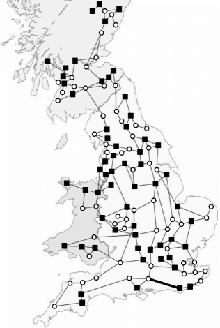
Figure 1: Topology of the power grid of the United Kingdom (UK) [29, 6, 21] with $N=120$ synchronous machines and $M=165$ transmission lines. Generators ($P_{i}>0$) are labeled ○and motors ($P_{i}<0$) denoted by ■. Half of the synchronous machines were chosen as generators and the other half as motors. The dashed line in the south-east denotes the transmission line $e_{\rm max}$ with the highest power flow $|K^{\rm flow}|=1.294$ which connects machines with powers $P_{117}=-0.76$ and $P_{118}=0.95$. After the removal of this edge the power flow in the transmission line depicted in bold (a bit to the west of the highest-flow line $e_{\rm max}$) increases most, actually it takes all the flow from $e_{\rm max}$ and it therefore defines the backup capacity $P_{\rm B}=1.294$. Map of the UK from [30], changed.

These backup capacities represent the resilience of a network against the failure of a transmission line. Note that the ability of a system to get back to stable operation after a single outage of a component (e.g., a transmission line) of a power grid is called $N-1$ criterion in electrical engineering. It is used in the planning and maintenance of power grids. Here, the backup capacities give an estimate of how much additional capacity of the transmission lines needs to be kept to keep them stable, even if one line breaks down. For small values of $P_{\rm B}$ the network structures are quite resilient, so few additional (over)capacity for the lines is needed. In case of large backup capacity the network structure does not allow to compensate a single-line failure so easily, therefore it is less resilient.

4 Networks

In this work we investigate one existing network and different network ensembles. We used the topology [29, 6, 21] of the British power grid (see figure 1) to determine the resilience of this grid when generators and motors are randomly placed on the nodes.

In addition, we obtained the pdf by means of a histogram of this resilience when one starts with the British grid with the same distribution of synchronous machines and uses the procedure for Erdős-Rényi graphs with fixed number of edges (cf., section 5). A more detailed discussion about figure 1 and the probability density function of the resilience is given in section 6.

The studied network ensembles are the Erdős-Rényi (ER) graph ensemble [31], and a spatial network ensemble [32]. The different parameters in these network models are chosen such that each node has (on average) three neighbors. This should take into account that real transmission grids are sparse with an average number of neighbors per node of $\langle k\rangle\approx 3$. For the North American power grid Kinney et al. [19] report about $N=14\,000$ substations and $M=20\,000$ transmission lines resulting in $\langle k\rangle\approx 2.9$. Watts and Strogatz [33] found for the the electrical power grid of the western U.S. $\langle k\rangle=2.67$. For the European transmission grid, Solé et al. [22] state a value of $\langle k\rangle=2.70$.

The simplest type of random network is an ER random graph. In this ER network ensemble [31] no assumptions on the topological structure of the network are made. It is therefore an ideal ensemble to be compared with, e.g., spatial networks to see the effects of topological structure. The creation of an ER network works as follows. One starts with an empty network of $N$ nodes. Then, each pair $i$, $j$ of nodes is connected with the probability

$$p_{ij}^{\rm ER}=c/N,$$ (9)

thus $c=\langle k\rangle=3$ is the connectivity of the network ensemble.

Next, we consider spatial networks [32] which are embedded in a two-dimensional plane. Each of the $N$ nodes is distributed uniformly at random in a $[0,1]\times[0,1]$-plane, so to each node a $x$- and a $y$-position are assigned. A link is added between nodes $i$ and $j$ with probability

$$p_{ij}^{\rm SN}=f\;\left(1+\sqrt{N\pi}\;d_{ij}/\alpha\right)^{-\alpha},$$ (10)

where $d_{ij}=[(x_{i}-x_{j})^{2}+(y_{i}-y_{j})^{2}]^{1/2}$ is the Euclidean distance between the two nodes. The parameters $f$ and $\alpha$ have been chosen such that an average number of neighbors $\langle k\rangle\approx 3$ is achieved. For all considered system sizes $N$ we used $\alpha=3$ and $f\in[0.54,1.9]$ (in decreasing order for increasing system size $N$).

In addition, we also used the ER ensemble with fixed number of links.

5 Simulation and reweighting method

To determine the pdfs over a large range of backup capacities for the different graph ensembles we use a reweighting technique. For details on the derivation of this technique we refer to [25, 34, 23] and state only the main ideas and results which are important for the determination of the pdf.

The main idea to reach very small probabilities or probability densities of the order $10^{-100}$ is the use of an additional Boltzmann factor $\exp(-P_{\rm B}(G)/T)$ in a Markov-chain Monte Carlo (MC) simulation generating network instances. This is different from simple sampling, where the network realizations are drawn directly and independently with their natural ensemble weights. The parameter $T$ is an artificial temperature, which makes it possible to sample different regions of the pdf of $P_{\rm B}$. The argument $G$ is the investigated network in the current MC step $t$.

This MC simulation works as follows. In each step $t$ of the simulation a candidate network $G^{*}$ from the current network $G(t)$ is created in the following way: First, a node $i$ is chosen uniformly at random. For the different network ensembles diverse techniques are now used. In the case of ER graphs all adjacent edges to $i$ are removed and with probability $p_{ij}^{\rm ER}=c/N$ a link is added for each other node $j$. For ER with a fixed number of edges also all adjacent edges to $i$ are removed. But next, node $i$ is connected with as many randomly chosen feasible nodes as removed edges. Hence, the number of edges is preserved. For spatial networks the procedure is the same as for ER graphs, but the probability to add a link is now $p_{ij}^{\rm SN}$ (see (10)).

Next, it is checked whether the graph $G^{*}$ is connected. If this is not the case, the above procedure is repeated on $G$ until a feasible network $G^{*}$ is found. Note that also the initial networks need to be connected. Therefore, ring-type or complete (all $N(N-1)/2$ edges present) networks are created in the beginning and the MC simulations with the above described procedure run until the desired connectivity is reached. For ER networks with fixed number of links the procedure for ER graphs with flexible number of links is used for this purpose.

After the candidate graph $G^{*}$ is created its backup capacity $P_{\rm B}$ is calculated. The candidate graph is then accepted ($G(t+1)=G^{*}$) with the Metropolis probability

$$p_{\rm Met}=\min\left\{1,\exp(-[P_{\rm B}(G^{*})-P_{\rm B}(G(t))]/T)\right\},$$ (11)

otherwise the current graph is kept ($G(t+1)=G(t)$).

From [25, 34, 23]

$$p(P_{\rm B})=\exp(P_{\rm B}/T)Z(T)p_{T}(P_{\rm B})$$ (12)

one can determine the full pdf $p(P_{\rm B})$ with pdfs $p_{T}(P_{\rm B})$ measured at different finite temperatures $T$ up to a normalization constant $Z(T)$. This constant can be determined by choosing two histograms of neighboring temperatures. In the overlapping region the pdfs need to agree which makes it possible to calculate $Z(T)$ via (12). In an iterative procedure the histograms are “glued” together until the full pdf is obtained. A more detailed explanation with examples about the merging of the different histograms is given in [35].

In order to check if the MC simulations are equilibrated, two different initial networks are used: A ring graph, where all nodes have two neighbors and a complete (fully connected) graph. Equilibration is reached when both values of $P_{\rm B}$ agree within the range of fluctuations. For the ensemble with fixed number of links, we studied the average of $P_{\rm B}$ over MC sweeps to determine the equilibration time. The longest equilibration time we observed was $2\cdot 10^{6}$ sweeps for ER networks with $N=50$ nodes.

6 Results

We performed simulations for the UK grid, ER networks, spatial networks and ER graphs with a fixed number of links. For all networks except the UK grid we used networks of size $N=10$ up to $N=400$. For ER and spatial graphs the determination of the (possibly) full pdf of the resilience for $N=400$ was not possible, as a large gap in this pdfs appeared. The histograms for different temperatures have their peak either below or above this gap, which made it almost impossible to sample in this gap. One way to overcome this is Wang-Landau sampling [36], which we did not try. Nevertheless, we took data also for these two ensembles for $N=400$ to analyse other quantities (see section 6.3).

After leaving out the data before equilibration time and taking samples only in intervals such that the Markov chain is roughly decorrelated, our final data sets contain between about $5\cdot 10^{3}$ samples for $N=400$ up to almost $10^{7}$ samples for $N=10$.

The consumed and produced powers $P_{i}$ are drawn from a uniform distribution $P_{i}\in[-1,1]$ and sum up to zero $\sum_{i}P_{i}=0$. Furthermore, a combination of $\{P_{i}\}$ is chosen, such that the same number of generators ($P_{i}>0$) and motors ($P_{i}<0$) are drawn. Most simply, sets of random numbers from the interval $[-1,1]$ were drawn until all above criteria can be fulfilled by assigning the last node. This is a bit time consuming, but has to be performed only once during a simulation: The power values attached to the nodes are not changed during the Markov-chain MC since all possible networks can be accessed just via changing the edges.

6.1 Probability density functions of the backup capacity

First, we analyze the probability density functions of the backup capacity for the different network ensembles as well as for the UK power grid.

Figure 2: (a) Probability density function $p(P_{\rm B})$ of the backup capacity $P_{\rm B}$ for ER networks with $N=120$ and $M=165$ (fixed) starting from the UK grid (see figure 1). About $10^{6}$ samples are used to generate this pdf.
(b) Scatter plot of the power flow $K_{e_{P_{\rm B}}}^{\rm flow}$ before the removal of the highest-load link through the edge which exhibits the highest flow increase (i.e., later defines the backup capacity) against the backup capacity $P_{\rm B}$ for $N=100$, an ER ensemble and $10^{5}$ samples. Dashed line represents $K_{e_{P_{\rm B}}}^{\rm flow}=P_{\rm B}$.

Figure 2(a) shows the pdf of the resilience for ER networks with a fixed number of links and $N=120$ nodes based on the UK grid (cf., figure 1). The procedure to create a candidate graph in the large-deviation scheme is the same as for ER graphs with a fixed number of edges (see section 5). Note that we only used one histogram with simple sampling corresponding to the temperature $T=\pm\infty$. Nevertheless, backup capacities from smaller than $0.4$ up to 2.8 could be measured. In figure 2(a) we can see an interesting double peak structure of the pdf, where the right peak is higher than the left. In these peaks the networks with typical values of the backup capacity are represented like the initial network of the simulation. A closer look to the two peaks reveals: Consider the power flow $K_{e_{P_{\rm B}}}^{\rm flow}$ before the removal of the highest-load link through the edge $e_{P_{\rm B}}$ which later defines the backup capacity, i.e., exhibits the highest flow increase. In figure 2(b), where $K_{e_{P_{\rm B}}}^{\rm flow}$ is plotted against the backup capacity, two clusters become visible: One cluster is represented by a very small flow through $e_{P_{\rm B}}$ before removal of $e_{\rm max}$ and quite high values of $P_{\rm B}$ (cluster below the dashed line). This cluster corresponds to the right (higher) peak of the pdf. An explanation for the left peak is that it belongs to the cluster, where a considerable flow through $e_{P_{\rm B}}$ is already present in the network and thus, the flow increase $P_{\rm B}$ is rather small (cigar-shaped cluster at small $P_{\rm B}$, many points above the dashed line).

The UK grid (see figure 1) has a backup capacity of $P^{*}_{\rm B}=1.294$ which is in this region of typical networks. Nevertheless, in principle much more resilient networks exist. This is confirmed by the $p$-value of the UK grid shown in figure 1. To obtain the $p$-value we calculate the cumulative probability that networks with smaller (or equal) backup capacity exist in the ensemble: $P(P_{\rm B}\leq P^{*}_{\rm B})\approx 0.67$. This value tells us that the probability of finding a more resilient network than the UK grid in the ER ensemble with fixed edges ($N=120$, $M=165$) is higher than 2/3. This means the UK grid as depicted in figure 1 has a low significance in terms of resilience, because of the large $p$-value. The right tail of the pdf follows an exponential resulting in a line in a logarithmic plot, whereas the left tail is much more curved.

Figure 3: (a) Probability density functions $p(P_{\rm B})$ of the backup capacity $P_{\rm B}$ for ER networks with sizes $N=10$ up to $N=200$. Inset: Region close to the peaks of the pdf for $N=10$ and $N=200$. Lines are guides to the eyes only.
(b) Peak positions $P_{\rm B}^{\rm peak}$ of the left peak in the pdfs for ER networks as a function of network size $N$. Dashed line is a logarithmic fit ($N=50$ excluded) $P_{\rm B}^{\rm peak}(N)=a\cdot\ln(b\cdot N)$ with parameters $a=0.146(8)$ and $b=0.44(6)$. Inset: The same for the right peak. The dashed line is a logarithmic fit ($N=50$ excluded) $P_{\rm B}^{\rm peak}(N)=c\cdot\ln(d\cdot N)$ with parameters $c=0.216(17)$ and $d=0.79(26)$.

Next, we compare the results for ER networks, spatial networks, and ER graphs with a fixed number of links. For all these ensembles we obtained the pdf over the possibly full support of $P_{\rm B}$. For many of the pdfs it was quite difficult to obtain the very left or very right tail. For very small values of the backup capacity (corresponding to small positive temperatures in the large-deviation approach) the histograms tend to become delta shaped, meaning the observable $P_{\rm B}$ becomes almost constant over MC time. The large values of the backup capacity (i.e., small negative temperatures) are even more difficult to obtain. In the simulations one could see that the maximum value of $P_{\rm B}$ could hardly be reached in the pdfs as sampling in this region results in a delta distribution. This is also visible in the finally obtained pdf (cf., e.g., figure 3(a)), because as the values of $P_{\rm B}$ get closer to the maximum a strong curvature appears.

Figure 3(a) shows the pdfs of the backup capacity for ER networks on almost the full support for different graph sizes $N$. In the inset of figure 3(a) the double-peaked structure of the pdfs for the smallest and the largest obtained networks are shown. For increasing graph size $N$ the double peaks shift towards larger backup capacities. We found that this shift is logarithmic in $N$ (cf., figure 3(b)). Interestingly, the right peak becomes more pronounced for $N=200$ in comparison to $N=10$.

With the large deviation approach described in section 5 one is able to access typical, very resilient and very vulnerable networks. Typical networks close to the double peaks of the pdfs show a rather small backup capacity. In figure 3(a) very vulnerable networks with a large backup capacity of $P_{\rm B}\approx 45$ for $N=200$ are very rare and appear only with a probability density of about $10^{-90}$. Note that such small probabilities (densities) are impossible to reach with ordinary MC simulations. These vulnerable networks are located at the right tail of the pdf. Although this tail is compatible with an exponential a strong curvature occurs when the maximum possible value of the backup capacity is approached. For transportation networks [23] the right tail of the pdf does not show any curvature. The very resilient networks can be found in the left tail close to the peaks of the density function.

(a) ER networks with fixed number of links and sizes $N=10$ up to $N=400$.

(b) Spatial networks with sizes $N=10$ up to $N=200$.

Figure 4: Probability density functions $p(P_{\rm B})$ of the backup capacity $P_{\rm B}$ for given networks. Inset: Region close to the peaks of the pdf for $N=10$ and $N=200$. Lines are guides to the eyes only.

In figure 4(a) the pdf for ER graphs with fixed number of edges is shown. Again, the peaks move logarithmically to the right with increasing $N$. Like for ER networks with variable number of links, the right of the two peaks is almost twice as high as the left peak for $N=200$. In contrast, for $N=10$ the peaks have almost the same height. The curvature of the right tail is not as strong as for ER or spatial networks.

Figure 4(b) shows the results for the spatial network model, where the nodes of the network are placed in a two-dimensional plane. As found for the other network ensembles the peaks in the inset of figure 4(b) shift logarithmically towards the right with growing number of nodes. The two peaks differ less in height for $N=200$ than for $N=10$. The curvature of the right tail is stronger than for the ER ensemble with fixed number of links.

Next, we compare the resiliences of typical, very vulnerable and very resilient networks for the different ensembles. For the typical networks we investigate the right (usually higher) peak of the pdf for $N=200$. For the ER network ensemble the typical networks exhibit a quite small backup capacity of $P_{\rm B}\approx 1.065$, followed by the ER ensemble with fixed number of links ($P_{\rm B}\approx 1.115$). Almost as resilient are the typical spatial networks with $P_{\rm B}\approx 1.163$. Similar results are found for the left peak.

Very vulnerable networks at $P_{\rm B}\approx 44$ for $N=200$ are most unlikely for the ER ensemble with fixed number of links ($p(P_{\rm B}\approx 44)\approx 10^{-106}$). For the ER ensemble this probability density at $P_{\rm B}\approx 44$ is about $10^{-88}$.

Networks from the spatial network ensemble have densities of about $10^{-82}$ at $P_{\rm B}\approx 44$. These results support the findings for the typical networks as for the two ER ensembles it is unlikely to find very vulnerable networks, i.e., with a large backup capacity. The graphs from the spatial network ensemble exhibit the highest densities at large backup capacities and thus favor less resilient networks.

Very resilient networks at $P_{\rm B}\approx 0.024$ for $N=200$ are most unlikely for the ER network ensemble with a fixed number of links, where $p(P_{\rm B}\approx 0.024)\approx 10^{-52}$. For the spatial ($p(P_{\rm B}\approx 0.024)\approx 10^{-37}$) and ER ($p(P_{\rm B}\approx 0.024)\approx 10^{-34}$) network ensemble the densities to find a network with $P_{\rm B}\approx 0.024$ are almost equal. In contradiction to what has been found previously, the ER ensemble with a fixed number of links exhibits quite low densities around $P_{\rm B}\approx 0.024$. Both spatial and ER network ensembles favor very resilient graphs, which have a small backup capacity.

These results need to be taken with care as for the ensemble with fixed number of edges arbitrarily small backup capacities can not be reached. In contrast, for the two ensembles with a flexible number of links many edges are allowed to be present in the networks and especially, the complete graph (each node is connected to all other nodes) is included in these ensembles. Therefore, the probability densities at low $P_{\rm B}$ for the ensembles with flexible number of links are of order $10^{18}$ higher than for the ER ensemble with fixed number of links.

To sum up, the most promising network ensemble in terms of resilience is the ER ensemble, although it is high dimensional, i.e., quite unrealistic. The ER ensemble with fixed number of links is also quite resilient against transmission line failure. The more realistic (it is embedded in a two-dimensional plane) spatial network ensemble is also a good candidate for choosing resilient networks, although vulnerable networks are quite likely. These findings are compatible with [23], although a much simpler very general transport model was studied there.

Figure 5: (a) Rate function $\Phi$ as a function of the rescaled backup capacity $r=P_{\rm B}/N$ for ER networks with fixed number of edges ($M=1.5N$) and different sizes $N$.
(b) Average backup capacity $P_{\rm B}$ as a function of the number of edges $N_{\rm e}$ for ER and spatial networks with size $N=400$.

6.2 The rate function

Next, we investigate the behavior of the so called rate function [37, 38]

$$\Phi=-\frac{1}{N}\log p(P_{\rm B}),$$ (13)

which describes that the leading behavior (away from the typical instances) of the pdf is an exponential decay $p(P_{\rm B})\sim e^{-NP_{\rm B}}$. Figure 5(a) shows the rate function as a function of the rescaled backup capacity $r=P_{\rm B}/N$ for the ER ensemble with fixed number of links. This rescaling is motivated by the following observation. Consider a network which consists of two large $\mathcal{O}(N)$ subnetworks which are connected via a core (e.g., a triangle, cf., [23]) with generators on one side and motors on the other. In this setup the most power has to flow through a single link of the core. After the removal of this high-loaded link, the power flows through the other two core links of the triangle. Hence, the backup capacity increases by an amount of $\sim N$, as the power flows of $N/2$ nodes run through these two links.

In figure 5(a) one sees that the rate function approaches a limiting curve as $N$ increases. Below a certain value $r=r^{*}$ this curve is approached from below, whereas above $r^{*}$ the curve is approached from larger values of $\Phi$. The point $r^{*}$ moves towards smaller values of $r$ as $N$ increases. For $N=400$ deviations from this behavior for large $r$ can be observed. Although the limiting curve is not compatible with a straight line as in [23], still an exponential behavior with strong curvature for $p(P_{\rm B})$ is possible.

Note that the rate functions for the other graph ensembles look similar with basically the same limiting behavior. This apparent convergence of the empirical rate function indicates that it might be promising to apply analytical large-deviation techniques [37, 38] to study resilience of power grids for these graph ensembles.

6.3 Characterization of very resilient and very vulnerable networks

Next, we investigate the relationship between the backup capacity, i.e., resilience and the number of edges in the graph for the ER and spatial network ensemble. Hence, we used our simulation results to bin data jointly for all different temperatures $T$ with respect to the number $N_{\rm e}$ of edges. In each of these bins the average backup capacity is calculated and the result is shown in figure 5(b). For a small number of edges in the network the backup capacity is very large. However, for many edges $P_{\rm B}$ assumes very small values. This means that in general a network with more edges is more resilient than a network with fewer edges. Note that adding a link to a network can sometimes destabilize it according to Braess’s paradox [39]. With our data it is not possible do determine whether the steep decrease of the backup capacity appears at smaller $N_{\rm e}$ for the ER or spatial network ensemble. In [23] the decrease appears at a smaller number of edges for the ER ensemble. Thus, in contrast to general transportation networks, it is possible to obtain very resilient power grids embedded in a two-dimensional plane with the same effort, i.e., number of edges, as for an infinite-dimensional, i.e., less restricted, ER ensemble.

(a) Average diameter $d$. Inset enlarges region for small $P_{\rm B}$.

(b) Average power sign ratio $p_{-}$.

Figure 6: Average diameter $d$ and power sign ratio $p_{-}$ as a function of the backup capacity $P_{\rm B}$ for all studied network ensembles with size $N=400$. Note that because of the gap in the data for ER and spatial networks some intermediate values of $P_{\rm B}$ are not present.

Figure 6(a) shows the average diameter for all studied network ensembles and $N=400$. The diameter of a network is defined as the longest of the shortest paths between all possible node pairs. First, a binning of the data with respect to the backup capacity is performed and afterwards the diameters are averaged within each bin. In the inset of figure 6(a) one can see that with increasing backup capacity the diameter also increases at least for small values of $P_{\rm B}$. Networks from the ER ensemble have the smallest diameter followed by networks from the ER ensemble with fixed number of links in this small $P_{\rm B}$ region. Networks from the spatial network ensemble reveal the largest diameters also for large backup capacities. Interestingly, graphs from the ER ensemble have a quite large diameter for larger backup capacities, whereas for smaller $P_{\rm B}$ the diameters are the smallest of all ensembles. These results are somehow opposite to what was found in [23], where networks from the spatial network ensemble reveal the smallest diameter for small backup capacities.

Networks from the ER ensemble with fixed number of edges show a decrease of the average diameter above $P_{\rm B}\approx 45$ and a small increase for very large backup capacities. This shows that the diameter is only a good observable to determine the resilience of a power flow network, if the edge number is flexible. Clearly, for real-world situations, where the number of links is an economic factor, one aims at minimal or at least constant edge number. Thus, for network ensembles with fixed number of edges other quantities may be considered.

One quantity is, e.g., what we call power sign ratio (cf., [9, 10], where a frequency sign ratio is used to characterize synchrony optimized networks). This quantity measures the fraction of links that connect synchronous machines whose power $P_{i}$ has opposite sign compared to the total number of edges in the network. In figure 6(b) the average of this quantity is shown for the studied network ensembles. The averaging is performed in the same way as for the graph diameter. For small $P_{\rm B}$ the power sign ratio is close to 0.5 for all network types. This means that on average from any two edges in the graph one of them connects machines with opposite signs of the power. This corresponds to the purely random case, since half of the nodes exhibit positive and half of the nodes negative power. Clearly, for increasing backup capacity, i.e., decreasing resilience $p_{-}$ also decreases. For networks from the spatial network ensemble this decrease is the most shallow.

Similarly to [9, 10], where a increasing value of the frequency sign ratio $p_{-}$ indicates enhancement of synchrony, here, $p_{-}$ (with the powers $P_{i}$) serves as a good indicator for the resilience of power flow networks.

7 Summary and outlook

We studied the resilience of power-flow models on networks against the failure of a transmission line. Three different random network ensembles, namely ER, spatial, and ER networks with fixed number of edges and the topology of the UK power grid were analyzed. The key quantity to determine the resilience of a network is the backup capacity. It is defined by the additional capacity of the links which needs to be provided for stable operation in case of a failure of the link with the highest power flow. This quantity is a realistic measure of resilience, since a power-grid blackout is very costly and should be avoided with a large effort. With a specific reweighting procedure the tails of the pdf below densities of $10^{-160}$ could be investigated. This allows for the study of very resilient and very vulnerable networks as well as typical ones. In addition, the $p$-value allows for the comparison of a given network with an network ensemble by giving a quality measure for the investigated network.

For the UK power grid we found a typical backup capacity $P_{\rm B}\approx 1.3$ which is located in the right peak of the corresponding pdf generated for an ER ensemble with fixed number of links. A $p$-value of 0.67 of the UK grid is indicating that it is of low significance with regard to resilience and that there exist many networks in the ER ensemble with fixed number of links that are more resilient. The position of the two peaks in the pdf increase logarithmically with growing $N$ for the three ensembles of random networks. The right tail of the pdfs for these three ensembles towards larger backup capacities is an exponential in about the left half of its support followed by a strong curvature in the right half of the support. This is confirmed by the rate function which converges to a corresponding limiting curve for increasing $N$.

Adding more links to a network makes it typically more resilient, which is not surprising. Also, in the non-spatial ER ensembles, which allow for more freedom when placing the edges, it is easier to find resilient networks. Nevertheless, for real applications, the two-dimensional model is more appropriate, in particular since it is almost as likely as for the ER ensembles to find very resilient networks. For this case more interestingly, resilient networks are characterized by a small diameter and a large power sign ratio even for the ER ensemble with fixed number of links. The latter observation is quite interesting, it means that power producers should be placed close to power consumers. This is convenient since this strategy reduces the costs for creating the network for transporting the electric power, as it is classically done anyway. Thus, minimizing the transportation costs and making the networks resilient are to a large extent not conflicting goals.

When using the $p$-value calculation, one should choose a suitable network ensemble for comparison. The ensemble should match the constraints of the investigated real-world network. Here, we used an ER ensemble with fixed number of edges for comparison with the UK grid as illustrating example. For practical evaluations of existing or planned power grids one would include, e.g., geographical constraints or cost minimization. Within such a constrained ensemble the backup capacity of an existing grid would be located in the low-probability tail of the pdf. Thus, a large-deviation approach, like presented here, is necessary to evaluate such a power grid.

In the future, it would be interesting to investigate more thoroughly where the double-peaked structure of the pdf comes from. It might also be useful to consider more realistic, i.e., dynamic, networks for electric power grids, as mentioned already above. In addition, one could use a spatial network ensemble which takes the costs of adding a transmission line into account to get an economically more realistic model.

References

References

- [1] Anderson P and Fouad A 2003 Power System Control and Stability 2nd ed (Piscataway, NJ, USA: IEEE Press, Wiley-Interscience)
- [2] Kundur P 1994 Power System Stability and Control (New York, NY, USA: McGraw-Hill)
- [3] Kuramoto Y 1984 Chemical oscillations, waves, and turbulence (New York, NY, USA: Springer-Verlag)
- [4] Kuramoto Y 1975 Int. Symp. on Mathematical Problems in Theoretical Physics (Lecture Notes in Physics vol 39) ed Araki H (New York, NY, USA: Springer) p 420
- [5] Filatrella G, Nielsen A and Pedersen N 2008 Eur. Phys. J. B 61 485
- [6] Rohden M, Sorge A, Timme M and Witthaut D 2012 Phys. Rev. Lett. 109(6) 064101
- [7] Magnesius H, Hirche S and Obradovic D 2012 American Control Conf. (Fairmont Queen Elizabeth, Montréal, Canada) p 2159
- [8] Dörfler F and Bullo F 2012 SIAM J. Contr. Optim. 50 1616
- [9] Brede M 2008 Phys. Lett. A 372 2618
- [10] Kelly D and Gottwald G A 2011 Chaos 21 025110
- [11] Barahona M and Pecora L M 2002 Phys. Rev. Lett. 89(5) 054101
- [12] Donetti L, Hurtado P I and Muñoz M A 2005 Phys. Rev. Lett. 95(18) 188701
- [13] Motter A E, Myers S A, Anghel M and Nishikawa T 2013 Nat. Phys. 9 191
- [14] Sachtjen M L, Carreras B A and Lynch V E 2000 Phys. Rev. E 61(5) 4877
- [15] Motter A E and Lai Y C 2002 Phys. Rev. E 66(6) 065102
- [16] Crucitti P, Latora V and Marchiori M 2004 Phys. Rev. E 69(4) 045104
- [17] Crucitti P, Latora V and Marchiori M 2004 Physica A 338 92
- [18] Chassin D and Posse C 2005 Physica A 355 667
- [19] Kinney R, Crucitti P, Albert R and Latora V 2005 Eur. Phys. J. B 46 101
- [20] Rosas-Casals M, Valverde S and Solé R V 2007 Int. J. Bifurcation Chaos Appl. Sci. Eng. 17 7
- [21] Simonsen I, Buzna L, Peters K, Bornholdt S and Helbing D 2008 Phys. Rev. Lett. 100(21) 218701
- [22] Solé R V, Rosas-Casals M, Corominas-Murtra B and Valverde S 2008 Phys. Rev. E 77(2) 026102
- [23] Hartmann A K 2014 Eur. Phys. J. B 87 114
- [24] Stott B, Jardim J and Alsac O 2009 IEEE Trans. Power Syst. 24 1290
- [25] Hartmann A K 2002 Phys. Rev. E 65(5) 056102
- [26] Moreno Y and Pacheco A 2004 Europhys. Lett. 68(4) 603
- [27] Coffrin C and Van Hentenryck P 2014 INFORMS J. Comp. 26(4) 718
- [28] Galassi M et al. 2009 GNU Scientific Library Reference Manual 3rd ed (Godalming: United Kingdom: Network Theory Limited) URL https://www.gnu.org/software/gsl/
- [29] Leigh J Map of the UK power grid URL https://www.deloitte.com/assets/Dcom-UnitedKingdom/Local%20As%sets/Documents/Industries/EIU/Gas%20and%20Power/uk-eiu-power-utilities-electricity.pdf
- [30] TUBS Map of the UK http://commons.wikimedia.org/wiki/File%3AUnited_Kingdom%2C_administrative_divisions_-_de_-_colored.svg via Wikimedia Commons license CC-BY-SA-3.0 (http://creativecommons.org/licenses/by-sa/3.0)
- [31] Erdős P and Rényi A 1960 Publ. Math. Inst. Hung. Acad. Sci. 5 17
- [32] Barthélemy M 2011 Phys. Rep. 499 1
- [33] Watts D and Strogatz S 1998 Nature 393 440
- [34] Hartmann A 2011 Eur. Phys. J. B 84 627
- [35] Hartmann A 2004 New Optimization Algorithms in Physics ed Hartmann A and Rieger H (Weinheim, Germany: Wiley-VCH) p 253
- [36] Wang F and Landau D P 2001 Phys. Rev. Lett. 86(10) 2050
- [37] den Hollander F 2000 Large Deviations (Providence, RI, USA: American Mathematical Society)
- [38] Touchette H 2009 Phys. Rep. 478 1
- [39] Witthaut D and Timme M 2012 New J. Phys. 14 083036