On Heterogeneous Neighbor Discovery
in Wireless Sensor Networks

Abstract

Neighbor discovery plays a crucial role in the formation of wireless sensor networks and mobile networks where the power of sensors (or mobile devices) is constrained. Due to the difficulty of clock synchronization, many asynchronous protocols based on wake-up scheduling have been developed over the years in order to enable timely neighbor discovery between neighboring sensors while saving energy. However, existing protocols are not fine-grained enough to support all heterogeneous battery duty cycles, which can lead to a more rapid deterioration of long-term battery health for those without support. Existing research can be broadly divided into two categories according to their neighbor-discovery techniques—the quorum based protocols and the co-primality based protocols. In this paper, we propose two neighbor discovery protocols, called Hedis and Todis, that optimize the duty cycle granularity of quorum and co-primality based protocols respectively, by enabling the finest-grained control of heterogeneous duty cycles. We compare the two optimal protocols via analytical and simulation results, which show that although the optimal co-primality based protocol (Todis) is simpler in its design, the optimal quorum based protocol (Hedis) has a better performance since it has a lower relative error rate and smaller discovery delay, while still allowing the sensor nodes to wake up at a more infrequent rate.

I Introduction

As human technology continues to advance at an unprecedented rate, there are more mobile wireless devices in operation than ever before. Many have taken advantage of the ubiquity of these devices to create mobile social network applications that use mobile sensing as an important feature [10][12]. These applications rely on their devices’ capability to opportunistically form decentralized networks as needed. For this to happen, it is important for these devices to be able to discover one another to establish a communication link. In order to save energy, each of the devices alternates between active and sleeping states by keeping its radio “ON” for only some of the time [4]. This is challenging to achieve because two nodes can communicate only when both of their radios are “ON” at the same time; and with clock drifts, having set times for all the nodes to wake up at the same time is not trivial. Since clock synchronization is difficult in a distributed system, neighbor discovery must be done asynchronously. Over the years, the asynchronous neighbor discovery problem has been widely studied [2][3][6][7][17][18][20], and existing research mainly focused on satisfying the following three design requirements:

1. Guarantee neighbor discovery within a reasonable time frame;

2. Minimize the number of time slots for which the node is awake to save energy;

3. Match the nodes’ awake-sleep schedules with their heterogeneous battery duty cycles as closely as possible to prolong overall battery lifetime.

Most existing solutions to this problem use patterned wake-up schedules to satisfy the first two requirements. We classify these solutions into two broad categories: (1) quorum based protocols that arrange the radio’s time slots into a matrix and pick wake-up times according to quorums in the matrix; and (2) co-primality based protocols that use numerical analysis to choose numbered time slots as the radio’s wake-up times.

In a quorum based protocol, a node populates time slots into a matrix, where the elements in the matrix represent time slots the node takes to run a period of the wake-up schedule [13]. The specific arrangements of rows and columns depends upon the protocol scheme, which typically assign slots as “active” or “sleeping”, such that it will ensure these chosen active time slots in the matrix of one node will overlap with those active ones of a neighboring node. Especially, when nodes have the same duty cycles, two nodes choosing active times from a row and a column respectively in the matrix will be ensured to achieve neighbor discovery regardless of clock drifts.

A co-primality based protocol directly takes advantage of properties of the Chinese Remainder Theorem (CRT) [11] to ensure that any two nodes would both be active in the same time slot [3]. Under these protocols, nodes wake up at time slots in multiples of chosen numbers (a.k.a. protocol parameters) that are co-prime to one another. Such a neighbor discovery protocol fails when nodes choose the same number that would compromise the co-primality. Thus, every node is allowed to choose several numbers and wake up at multiples of all of those chosen numbers, which guarantees that nodes discover one another within a bounded time/delay.

Up to now, all of the protocols incepted, be it quorum based or co-primality based, fail to meet the third design requirement, as their requirements for duty cycles are too specific. As a quorum based protocol, Searchlight [2] requires that the duty cycles be in the form $\frac{2}{n^{i}}$, where $n$ is a fixed integer (it only supports duty cycles of $1,\frac{1}{2},\frac{1}{4},\frac{1}{8},\frac{1}{16},\ldots$ if $n=2$). Therefore, it greatly restricts the choices of supported duty cycles due to the requirement of power-multiples of $2/n$. For a co-primality based protocol like Disco [3], it restricts duty cycles to be in the form $\frac{1}{p_{1}}+\frac{1}{p_{2}}$, where $p_{1}$ and $p_{2}$ are prime numbers. Such stringent requirements on duty cycles force devices to operate at duty cycles that they are not designed to operate at, thus shortening their longevity.

In this paper, we present two optimal neighbor discovery protocols, called Hedis (HEterogeneous DIScovery as a quorum based protocol) and Todis (Triple-Odd based DIScovery as a co-primality based protocol), that guarantee asynchronous neighbor discovery in a heterogeneous environment, meaning that each node could operate at a different duty cycle. Specifically, they optimize the duty cycle granularity in their respective protocol categories to support duty cycles in the form of $\frac{2}{n}$ and $\frac{3}{n}$ respectively, and $n$ is an integer that help achieve almost all duty cycles smaller than one. We analytically compare these two protocols with existing state-of-the-art protocols to confirm their optimality in the support of duty cycles, and also compare them against each other as a comparison between the two general categories of neighbor discovery protocols (quorum vs. co-primality based protocols). Our results show that while the discovery latencies are similar for both protocols, Hedis as an optimal quorum based protocol matches actual duty cycles much more closely than Todis as a co-prime based protocol.

The rest of this paper is organized as follows. We formally define the problem as well as any necessary terms in section II, and give a taxonomy of current research efforts in this area in section III. In sections IV and V, we present our optimizations for the quorum based and co-primality based protocols respectively, and we evaluate them with simulations in section VI. Finally, we conclude with section VII.

II Problem Formulation

Here we define the terms and variables used to formally describe the neighbor discovery problem and its solution, as well as state any assumptions used in devising our protocols.

Wake-up schedule. We consider a time-slotted wireless sensor network where each node is energy-constrained. The nodes follow a neighbor discovery wake-up schedule that defines the time pattern of when they need to wake up (or sleep), so that they can discover their respective neighbors in an energy-efficient manner.

Definition 1.

The neighbor discovery schedule (or simply schedule) of a node $a$ is a sequence $\mathbf{s}_{a}\triangleq\{s_{a}^{t}\}_{0\leq t<T_{a}}$ of period $T_{a}$ and

$$s_{a}^{t}=\begin{cases}0&\text{$a$\leavevmode\nobreak\ sleeps in slot $t$}\\ 1&\text{$a$\leavevmode\nobreak\ wakes up in slot $t$}\end{cases}.$$

Clock drift. We do not assume clock synchronization among nodes, therefore any two given nodes may have random clock drifts. We use the cyclic rotation of a neighbor discovery schedule to describe this phenomenon. For example, a clock drift by $k$ slots of node a’s schedule $s_{a}$ is

$$rotate(\mathbf{s}_{a},k)=\{r_{a}^{t}\}_{0\leq t<T_{a}},$$

where $r_{a}^{t}=s_{a}^{(t+k)\bmod T_{a}}$.

Definition 2.

The duty cycle $\delta_{a}$ of node $a$ is the percentage of time slots in one period of the wake-up schedule where node $a$ is active (node $a$ wakes up), defined as

$$\delta_{a}=\frac{|\{0\leq t<T_{a}:s_{a}^{t}=1\}|}{T_{a}}.$$

Neighbor discovery. Suppose two nodes $a$ and $b$ have schedules $\mathbf{s}_{a}$ and $\mathbf{s}_{b}$ of periods $T_{a}$ and $T_{b}$, respectively. If $\exists t\in[0,\textrm{lcm}(T_{a},T_{b}))$ such that $\mathbf{s}_{a}^{t}=\mathbf{s}_{b}^{t}=1$ where $\textrm{lcm}(T_{a},T_{b})$ is the least common multiple of $T_{a}$ and $T_{b}$, we say that:

• Nodes $a$ and $b$ can discover each other in slot $t$.

• Slot $t$ is called the discovery slot between $a$ and $b$.

Figure 1 shows an example of two nodes with neighbor discovery schedules $\mathbf{s}_{a}=\{0,0,0,0,0,1\}$ and $\mathbf{s}_{b}=\{0,1,0,0,0,0,0,0,1\}$, that have period lengths of $T_{a}=6$ and $T_{b}=9$ respectively. Node $a$ is active on 1 slot within each period (6 slots) while node $b$ is active on 2 slots within each period (9 slots). Thus the duty cycles of $a$ and $b$ are $d_{a}=\frac{1}{6}\approx 16.7\%$ and $d_{b}=\frac{2}{9}\approx 22.2\%$. In Figure 1(a), We see that for every period of 18 slots ($\textrm{lcm}(T_{a},T_{b})=18$), nodes $a$ and $b$ discover each other in slot 17. However, as illustrated in Figure 1(b), when a one-slot clock drift occurs in node $b$, we have $rotate(\mathbf{s}_{b},1)=\{1,0,0,0,0,0,0,1,0\}$ and these two nodes can no longer discover each other.

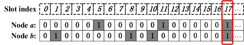
(a) Without clock drift

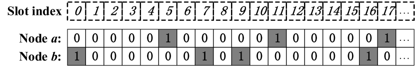
(b) Node $b$ drifts by 1 time slot to the left

Figure 1: An example of neighbor discovery: Two neighbor discovery schedules are $\mathbf{s}_{a}=\{0,0,0,0,0,1\}$ and $\mathbf{s}_{b}=\{0,1,0,0,0,0,0,0,1\}$. Without clock drift (1(a)), the two nodes can discover each other every 18 time slots since $\textrm{lcm}(T_{a},T_{b})=18$. With clock drift (1(b)), neighbor discovery fails.

III A Taxonomy of Neighbor Discovery Protocols

In this section, we introduce a taxonomy of deterministic asynchronous neighbor discovery protocols. Through examining existing solutions to the neighbor discovery problem, we divide these protocols into two broad categories.

III-A Why Deterministic Protocols

Many solutions have been proposed to solve the neighbor discovery problem. One of the earliest such solutions are the birthday protocols [9], which take upon a probabilistic approach to neighbor discovery. These protocols rely on the birthday paradox, which states that with as few as 23 people, the probability that two people have the same birthday exceeds $\frac{1}{2}$. As a non-deterministic protocol based upon probability, birthday protocols are heterogeneous and supports every duty cycle with the finest granularity. Following this, many more similar probabilistic protocols were also developed [14][15][16][19]. However, due to their probabilistic nature, these protocols fail to provide a guaranteed upper bound for neighbor discovery latency, which means that there is a chance for two neighbors to never discover each other.

To combat this insufficiency, deterministic protocols with worst case bounds for neighbor discovery were developed. The earlier deterministic protocols such as [6][13], and [8] all use the quorum concept. However, while these protocols are effective in guaranteeing neighbor discovery, they are generally lacking in duty cycle support. For example, [13] and [6] are homogeneous, meaning that they require all the nodes to have the same duty cycle. As a result, the co-primality based approach was developed with Disco [3] and U-Connect [7], although U-Connect is in some ways a hybrid approach using elements from both the quorum and co-primality paradigms.

III-B Quorum vs. Co-primality Based Protocols

The deterministic protocols for neighbor discovery can be largely classified into two major categories, quorum based protocols and co-primality based protocols, though they both work because of the CRT.

III-B1 Quorum Based Protocols

Quorum based protocols take advantage of geometry in a 2-dimensional array.

Bounded discovery delay. In the most original protocols like [13], time is arranged into an $m\times m$ matrix. Every node then chooses a row and a column for which to wake up. This ensures that regardless of any clock drifts, any two nodes would be able to wake up at the same time slot at least twice every $m^{2}$ time slots, thus guaranteeing an upper bound for neighbor discovery. However, this method only works if every node happens to use the same duty cycle. Lai et al. [8] improve upon this method by constructing cyclic quorum system and grid quorum system pairs, which allow for two different duty cycles to coexist and still ensure bounded neighbor discovery.

Example protocols. The current latest development in quorum based protocols is Searchlight [2], which is able to support multiple duty cycles in the network. Searchlight essentially divides the duty cycle period into a $\frac{t}{2}\times t$ matrix, and uses a combination of anchor and probing slots to generate wake up patterns. At the beginning of every $t$ time slots is an anchor slot, and a probing slot occurs at random slots between the anchor slots. With this technique, Searchlight [2] shows that it is able to allow neighbor discovery among nodes with many different duty cycles.

III-B2 Co-primality Based Protocols

A co-primality based neighbor discovery protocol is one in which

• Each node, say, node $a$, chooses a set of integers (not necessarily distinct) $N_{a}=\{n_{1}^{a},n_{2}^{a},n_{3}^{a},\ldots,n_{|N_{a}|}^{a}\}$.

• For two distinct nodes $a$ and $b$, $N_{a}$ and $N_{b}$ must satisfy the following co-prime pair property.

Definition 3.

For two distinct nodes $a$ and $b$ under a co-primality based neighbor discovery protocol, there exists an integer in $N_{a}$ that is co-prime to an integer in $N_{b}$—i.e., $\exists n_{i_{0}}^{a}\in N_{a}$ and $n_{j_{0}}^{b}\in N_{b}$ such that $n_{i_{0}}^{a}$ and $n_{j_{0}}^{a}$ are co-prime.

Node $a$’s schedule $\mathbf{s}_{a}\triangleq\{s_{a}^{t}\}_{0\leq t<T_{a}}$ under this co-primality based protocol is

$$s_{a}^{t}=\begin{cases}1&t\,\mbox{is divisible by some $n_{i}^{a}\in N_{a}$}\\ 0&\text{otherwise}\end{cases}.$$

The period length is $T_{a}=\textrm{lcm}(n_{1}^{a},n_{2}^{a},\ldots,n_{|N_{a}|}^{a})$ and its duty cycle $\delta_{a}$ is

$$\delta_{a}=\sum_{1\leq i_{1}\leq|N_{a}|}\frac{1}{n_{i_{1}}^{a}}-\sum_{1\leq i_{1}<i_{2}\leq|N_{a}|}\frac{1}{\textrm{lcm}(n_{i_{1}}^{a},n_{i_{2}}^{a})}$$

$$\cdots+(-1)^{|N_{a}|+1}\frac{1}{\textrm{lcm}(n_{1}^{a},n_{2}^{a},n_{3}^{a},\cdots,n_{|N_{a}|}^{a})}.$$

Bounded discovery delay. By the Chinese Remainder Theorem (CRT) [11], we can obtain the following theorem.

Theorem 4.

A co-primality based neighbor discovery protocol can guarantee discovery for any two nodes for any amount clock drift if the associated integer sets of the nodes in this network satisfy the co-prime pair property. And the worst-case discovery delay is bounded by the product of the two smallest co-prime numbers, one from each set, i.e.:

$$\min_{\textrm{gcd}(n_{i}^{a},n_{j}^{b})=1,1\leq i\leq N_{a},1\leq j\leq N_{b}}\{n_{i}^{a}\cdot n_{j}^{b}\}.$$

Suppose the clock of node $a$ is $d$ time slots ahead of that of node $b$, i.e., node $b$’s $t^{th}$ time slot is the $(t+d)^{th}$ time slot of node $a$, where $d$ is the clock drift, the following congruence system w.r.t. $t$ applies:

$$\begin{cases}t\equiv 0&\pmod{p_{i}}\\ t+d\equiv 0&\pmod{p_{j}}\end{cases}.$$ (1)

If $t$ is a solution to Eq. (1), then node $a$ will discover node $b$ in node $a$’s $t$-th time slot (i.e., node $b$’s $(t+d)$-th time slot). By CRT, since $p_{i}$ and $p_{j}$ are co-prime, there exists a solution $t\equiv t_{0}\pmod{p_{i}p_{j}}$.

Example protocols. Disco [3], as such a co-primality based protocol, ensures co-primality by only using prime numbers as possible parameters. In Disco, each node chooses two distinct primes to create its wake-up schedule. For example, node $a$ chooses two distinct primes $p_{1}$ and $p_{2}$ and node $b$ chooses $p_{3}$ and $p_{4}$. Node $a$ is active (wakes up) in the $t$-th time slot iff $t$ is divisible by either $p_{1}$ or $p_{2}$ while node $b$ is active in the $t$-th time slot iff $t$ is divisible by either $p_{3}$ or $p_{4}$. Therefore, Disco can guarantee neighbor discovery for any two nodes for any amount of clock drift with a bounded discovery delay of

$$\min_{\textrm{gcd}(p_{i},p_{j})=1,i=1,2,j=3,4}\{p_{i}\cdot p_{j}\}.$$

Again, this delay is the product of the two smallest co-prime numbers following from the CRT.

U-Connect [7] is a combination of Disco and the basic quorum based protocol in that it restricts the dimensions of the square quorum matrix to be a prime number. In this way, if the duty cycles of the nodes happen to be the same, neighbors would discover one another via the quorum method. On the other hand, if they are different, the numbers chosen would be co-prime to each other and thus enabling neighbor discovery by Theorem 4.

More comprehensive surveys on neighbor discovery can be found in [1] and [5].

IV Hedis: Optimizing the Quorum based Protocols

Hedis is an asynchronous periodic slot-based neighbor discovery protocol where each node picks its anchor and probing slots according to the elements of a quorum that is carefully selected in an $(n-1)$ by $n$ matrix.

IV-A Design of the Hedis Schedule

For a node $a$ that has a desired duty cycle $\delta$, the period of its schedule under Hedis, $\mathbf{s}_{a}=\{s_{a}^{t}\}_{0\leq t<n(n-1)}$, consists of $n(n-1)$ time slots, where the integer $n$ is chosen such that $\frac{2}{n}$ comes as close to $\delta$ as possible (and we call $n$ the parameter of this node). Under Hedis, its schedule is

$$s_{a}^{t}=\begin{cases}1&t=ni,(n+1)i+1\text{ (}i=0,1,2,\ldots,n-2\text{)}\\ 0&\text{otherwise}\end{cases},$$

where $ni$ ($i=0,1,2,\ldots,n-2$) denotes the index of an anchor slot and $(n+1)i+1$ denotes the index of a probing slot.

Figure 2 shows two example Hedis schedules when $n=4,6$, and the two schedules consist of of $n(n-1)=12,30$ time slots, respectively. Each grid in the figure represents a time slot, and the integer inside a grid denotes its slot index, e.g., the grid with $0$ inside denotes the 0th time slot in the schedule (note that a schedule starts from the 0th time slot). The red and blue slots represent the anchor and probing slots, during which the node wakes up. When $n=4$, the duty cycle is $2/4=50\%$. The full schedules are depicted in Figure 3, where the two nodes with different duty cycles can achieve successful neighbor discovery (overlap of colored slots between schedules of nodes $a$ and $b$) for many times in every period. Next, we will show that Hedis can guarantee neighbor discovery for any two nodes of same-parity parameters (both odd or both even) with heterogeneous duty cycles for any amount of clock drift.

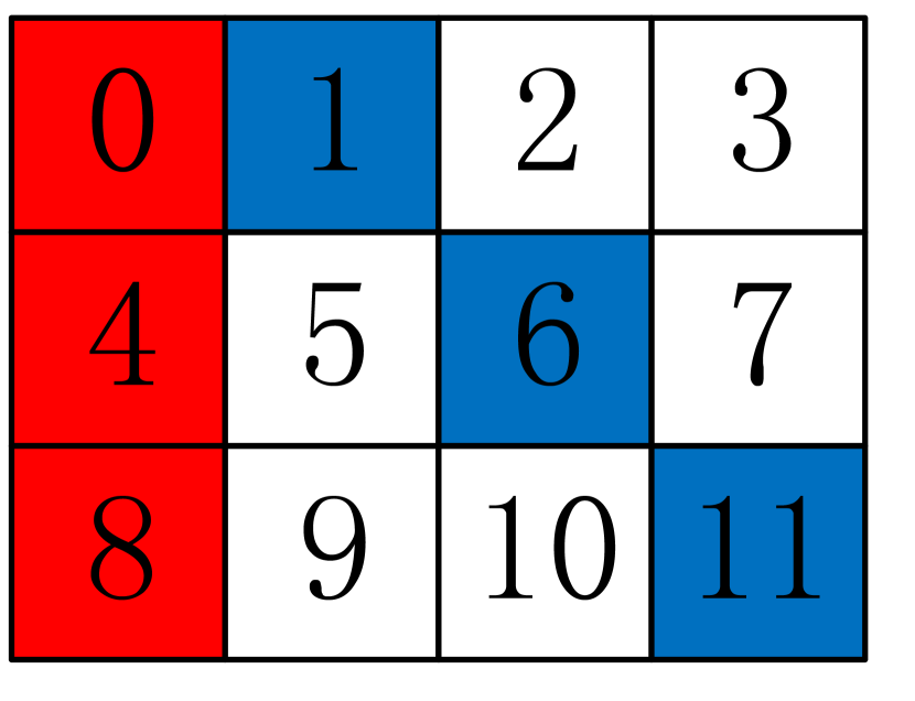
(a) n=4

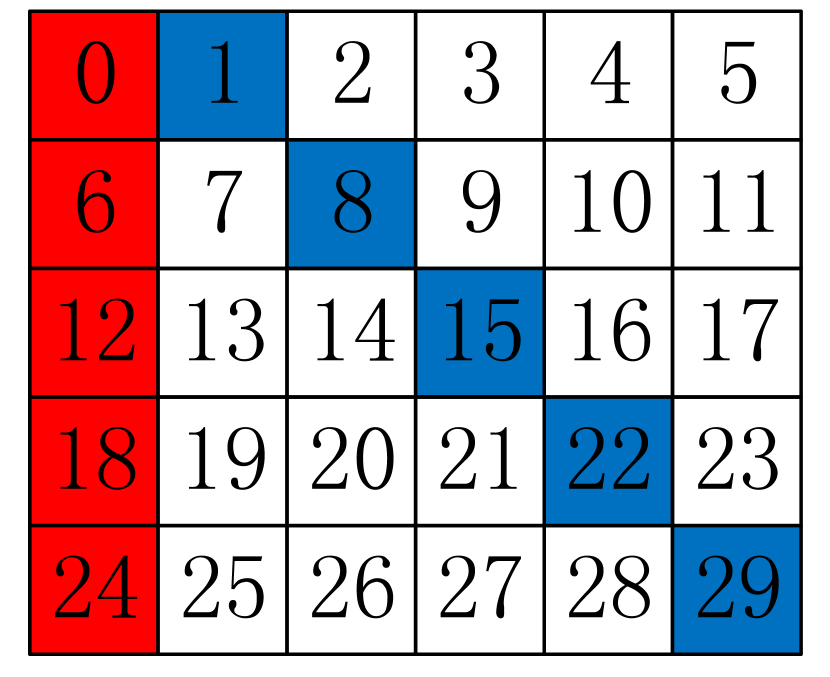
(b) n=6

Figure 2: Two example Hedis schedules.

Figure 3: Node $a$’s schedule is 3-slot ahead of node $b$’s schedule. The overlapped colored slots between their schedules represent the successful neighbor discovery.

IV-B Bounded Discovery Delay under Hedis

Lemma 5.

Let $m$ and $n$ be positive integers. For any integers $a$ and $b$, there exists an integer $x$ such that

$$x\equiv a\pmod{m}$$ (2)

and

$$x\equiv b\pmod{n}$$ (3)

if and only if

$$a\equiv b\pmod{\text{gcd}(m,n)}.$$

If $x$ is a solution of congruences (2) and (3), then the integer $y$ is also a solution if and only if

$$x\equiv y\pmod{\text{lcm}(m,n)}.$$

The proof can be found in [11], on page 61, Theorem 2.9. By Lemma 5, we further establish the following theorem.

Theorem 6.

Hedis guarantees neighbor discovery within bounded latency for any two nodes with the same-parity parameters $n$ and $m$, given any amount of clock drift between their schedules. The average discovery latency is $O(nm)$.

Proof:

Nodes $a$ and $b$ are two arbitrarily given nodes, whose parameters are $n$ and $m$, respectively. The periods of the Hedis schedules of nodes $a$ and $b$ are $T_{a}=n(n-1)$ and $T_{b}=m(m-1)$, respectively. We use $d$ to denote the clock drift.

Without loss of generality, we study the following system of congruences with respect to $t$:

$$\begin{cases}t\equiv ni+d,(n+1)i+1+d\pmod{n(n-1)}\\ t\equiv mj,(m+1)j+1\pmod{m(m-1)},\end{cases}$$ (4)

where $i\in[0,n-2]$, $j\in[0,m-2]$.

$$t\equiv ni+d,(n+1)i+1+d\pmod{n(n-1)}$$

($i\in[0,n-2]$) is true iff $\exists i\in[0,n-2]$ such that it is true, and the same meaning for

$$t\equiv mj,(m+1)j+1\pmod{m(m-1)}$$

($j\in[0,m-2]$).

There are a number of $nm$ pairs of simultaneous congruences, which we divide into 4 groups: anchor-anchor, anchor-probing, probing-anchor and probing-probing groups. E.g., the anchor-probing group denotes the case where an anchor slot of node $a$ overlaps a probing slot of node $b$. Note that if we find a solution that meets the requirements of any one of these congruences, we obtain a solution to Eq. (4).

Group 1: anchor-anchor. Consider the following system of congruences

$$\begin{cases}t\equiv ni+d\pmod{n(n-1)}&i\in[0,n-2]\\ t\equiv mj\pmod{m(m-1)}&j\in[0,m-2]\end{cases},$$

which is equivalent to

$$\begin{cases}t\equiv d\pmod{n}\\ t\equiv 0\pmod{m}\end{cases}.$$ (5)

By Lemma 5, Eq. (5) has a solution if and only if

$$\textrm{gcd}(n,m)\mid d.$$

Group 2: anchor-probing. Consider the following system of congruences

$$\begin{cases}t\equiv ni+d\pmod{n(n-1)}&i\in[0,n-2]\\ t\equiv(m+1)j+1\pmod{m(m-1)}&j\in[0,m-2]\end{cases},$$ (6)

which is equivalent to

$$\begin{cases}t\equiv d\pmod{n}\\ t\equiv(m+1)j+1\pmod{m(m-1)}&j\in[0,m-2]\end{cases}.$$ (7)

By Lemma 5, Eq. (7) has a solution if and only if $\textrm{gcd}(n,m(m-1))\mid(m+1)j+1-d$ for some integer $j\in[0,m-2]$, i.e., the congruence with respect to $j$

$$(m+1)j\equiv d-1\pmod{\textrm{gcd}(n,m(m-1))}$$ (8)

has a solution.

Group 3: probing-anchor. Consider the following system of congruences

$$\begin{cases}t\equiv(n+1)i+1+d\pmod{n(n-1)}&i\in[0,n-2]\\ t\equiv mj\pmod{m(m-1)}&j\in[0,m-2]\end{cases},$$ (9)

which is equivalent to

$$\begin{cases}t\equiv(n+1)i+1+d\pmod{n(n-1)}&i\in[0,n-2]\\ t\equiv 0\pmod{m}\end{cases}.$$ (10)

By Lemma 5, Eq. 10 has a solution if and only if

$$\textrm{gcd}(m,n(n-1))\mid(n+1)i+1+d$$

for some integer $i\in[0,n-2]$, i.e., the congruence with respect to $i$

$$(n+1)i\equiv-d-1\pmod{\textrm{gcd}(m,n(n-1)}$$

has a solution.

Group 4: probing-probing. Consider the following system of congruences

$$\begin{cases}t\equiv(n+1)i+1+d\pmod{n(n-1)}&i\in[0,n-2]\\ t\equiv(m+1)j+1\pmod{m(m-1)}&j\in[0,m-2]\end{cases}.$$ (11)

By Lemma 5, Eq. 11 has a solution if and only if

$$\textrm{gcd}(n(n-1),m(m-1))\mid(n+1)i-(m+1)j+d$$

for some integer $i\in[0,n-2]$ and $j\in[0,m-2]$.

Now we begin to prove this theorem by cases.

Case 1: If $m>n$, the congruence system of anchor-probing (Group 2) is true. Proof: If $m>n$, we have $m-1\geq n\geq\textrm{gcd}(n,m(m-1))$. And note that $\textrm{gcd}(m+1,\textrm{gcd}(n,m(m-1)))=\textrm{gcd}(m+1,n,m(m-1))=\textrm{gcd}(m+1,2,n)=1$. This is because $m$ and $n$ are both odd or are both even. So one of $m+1$ and $n$ are odd, and we have $\textrm{gcd}(m+1,2,n)=1$. Therefore $(m+1)j$ ($j\in[0,m-2]$) runs over all congruence classes modulo $\textrm{gcd}(n,m(m-1))$. Then Eq. (8) has at least $\lfloor(m-1)/\textrm{gcd}(n,m(m-1))\rfloor$ solutions and on average $(m-1)/\textrm{gcd}(n,m(m-1))$ solutions. Hence Eq. (7) has at least $\lfloor(m-1)/\textrm{gcd}(n,m(m-1))\rfloor$ solutions and on average $(m-1)/\textrm{gcd}(n,m(m-1))$ solutions modulo $\textrm{lcm}(n,m(m-1))$. Therefore, the average discovery latency is $\frac{\textrm{lcm}(n,m(m-1))}{(m-1)/\textrm{gcd}(n,m(m-1))}=nm$.

Case 2: If $n>m$, the congruence system of probing-anchor (Group 3) is true. Proof: If $n>m$, similarly to case 1, we have Eq. (10) has at least $\lfloor(n-1)/\textrm{gcd}(m,n(n-1))\rfloor$ solutions and on average $(n-1)/\textrm{gcd}(m,n(n-1))$. Hence Eq. (9) has at least $\lfloor(n-1)/\textrm{gcd}(m,n(n-1))\rfloor$ solutions and on average $(n-1)/\textrm{gcd}(m,n(n-1))$ modulo $\textrm{lcm}(m,n(n-1))$. Therefore, the average discovery latency is $nm$.

Case 3. If $n=m$, we consider the result of $d\bmod n$. If $d\equiv 0\pmod{n}$, then $\textrm{gcd}(n,m)=n\mid d$, and thus the anchor-anchor case (Group 1) is true and the average discovery latency is $O(nm)$. Now we concentrate on the case where $d\not\equiv 0\pmod{n}$. Since $n=m$, Eq. (8) becomes

$$(n+1)j\equiv d-1\pmod{n}.$$

Since $(n+1)j=nj+j\equiv j\pmod{n}$, this is equivalent to

$$d\equiv j+1\pmod{n}.$$

For $j\in[0,n-2]$, $j+1$ runs over$[1,n-1]$. Because $d\not\equiv 0\pmod{n}$, there exists a $j\in[0,n-2]$ that satisfies Eq. (8), and therefore the anchor-probing case (Group 2) is true. Similarly, the probing-anchor case (Group 3) is also true. And it is easy to check that the average discovery latency is $O(n^{2})$, i.e., $O(nm)$. ∎

V Todis: Optimizing Co-primality based Protocols

Now we optimize the asynchronous co-primality based protocols, and propose Todis that exploits properties of consecutive odd integers for achieving co-primality.

As a co-primality based protocol, Todis creates wake-up schedules for the nodes based on multiples of numbers that are co-prime to each other. This ensures that any two given nodes would be able to wake up at the same time by the co-prime pair property as illustrated in Section III, thus succeeding in neighbor discovery. Recall that Disco [3] guarantees this by simply using prime numbers as parameters, which limits the variety of parameters to choose from.

For two nodes $a$ and $b$, we need to construct two sets of integers, $N_{a}$ and $N_{b}$, that must satisfy the co-prime pair property. In our quest to find co-prime pairs, we observe that for two numbers to be co-prime, at least one of them must be odd. Thus, we explore the possibility of achieving co-primality using odd integers. We observe that given two odd integers $a$ and $b$, if they are not co-prime, often times either “$a+2$ and $b$”, or “$a$ and $b+2$” is a co-prime pair. For example, if 15 and 21 are not co-prime, we are able to find that either “17 and 21”, or “15 and 23” is a a co-prime pair. Following this logic, we design our Todis protocol using sets of consecutive integers.

V-A Design of the Todis Schedule

V-A1 Trying sets of two consecutive integers

First, we tried using two consecutive odd integers in $N_{a}$ for each node $a$, i.e., $N_{a}=\{n,n+2\}$ where $n\geq 1$ and $n$ is odd. Unfortunately, for given nodes $a$ and $b$, there are instances where the sets $N_{a}$ and $N_{b}$ do not satisfy the co-prime pair property for very small numbers (i.e., less than 100). For example, when $N_{a}=\{33,35\}$ and $N_{b}=\{75,77\}$ and $\forall n_{i}^{a}\in N_{a},n_{j}^{b}\in N_{b}$, we have $\textrm{gcd}(n_{i}^{a},n_{j}^{b})>1$.

V-A2 Using sets of three consecutive integers in Todis

In Todis, we use three consecutive odd integers $n-2$, $n$ and $n+2$ ($n\geq 3$) for constructing a wake-up schedule.

The co-prime pair property requires that at least one of the three consecutive odd integers that node $a$ chooses (i.e., $n-2$, $n$ and $n+2$) is co-prime w.r.t. one of the three integers that node $b$ chooses (i.e., $m-2$, $m$ and $m+2$).

Bounded discovery delay in practical networks. Generally, the triples consisting of three consecutive odd integers can also fail to satisfy the required co-prime pair property, as seen in counterexamples shown by the CRT. However, the two smallest sequences of odd integers in these counterexamples are $N_{a}=\{1600023,1600025,1600027\}$ and $N_{b}=\{2046915,2046917,2046919\}$. Such integers are too large to be chosen for creating a “practical” duty cycle anyway. For example, an $n$ value larger than $1600023$ would imply a duty cycle smaller than $\delta_{a}$ of $0.00000187496$. In practical applications, however, duty cycles are much greater than $0.00000187496$. Therefore, any chosen sets $N_{a}$ and $N_{b}$ based on duty cycles would satisfy the co-prime pair property. By Theorem 4, Todis guarantees neighbor discovery with a delay bounded by

$$\min_{\textrm{gcd}(n+i,m+i)=1,i=-2,0,2}\{n\cdot m\}.$$

A node $a$ that has a desired duty cycle of $\delta$ may therefore choose an odd integer $n$ such that

$$\frac{3(n^{2}-n-1)}{n(n^{2}-4)}\approx\frac{3}{n}=\hat{\delta}$$

is as close to $\delta$ as possible. We call $n$ the parameter of node $a$.

Under Todis, its wake-up schedule is

$$s_{a}^{t}=\begin{cases}1&t\leavevmode\nobreak\ \mbox{is divisible by either $n-2$, $n$, or $n+2$}\\ 0&\text{otherwise}\end{cases},$$

with a period length of $(n-2)n(n+2)$ and a duty cycle of

$$\frac{1}{n-2}+\frac{1}{n}+\frac{1}{n+2}-\frac{1}{(n-2)n}-\frac{1}{n(n+2)}-\frac{1}{(n-2)(n+2)}$$

$$+\frac{1}{(n-2)n(n+2)}=\frac{3(n^{2}-n-1)}{n(n^{2}-4)}.$$

Figure 4 shows the first 71 time slots under the Todis schedule when $n=15$ (i.e., the node chooses $13$, $15$ and $17$). Each grid in the figure represents a time slot, and the integer inside a grid denotes its slot index, e.g., the grid with $0$ inside denotes the 0th time slot in the schedule (note that a schedule starts from the 0th time slot). The gray slots represent the active slots where the node wakes up. In this example, the duty cycle is $\frac{3\cdot(5^{2}-5-1)}{5\cdot(5^{2}-4)}\approx 18.9\%$.

Figure 4: The first 71 time slots under the Todis schedule when $n=15$ (i.e., the node chooses $13$, $15$ and $17$). The node wakes up in time slots 0, 13, 15, 17, 26, 30, 34, 39, 45, 51, 52, 60, 68, $\ldots$.

V-B Analysis of Duty Cycle Granularity

Now we discuss the granularity of Todis in matching any desired duty cycle in practical applications. Suppose node $a$’s desired duty cycle is $\delta_{a}$, the relative error $\epsilon(\delta_{a})$ between $\delta_{a}$ and its approximation $\hat{\delta_{a}}$ is defined by

$$\epsilon(\delta_{a})=\frac{\left|\hat{\delta}_{a}-\delta_{a}\right|}{\delta_{a}}.$$ (12)

We want to mathematically estimate the upper bound of $\epsilon$ given $\delta_{a}$, which we denote as $\hat{\epsilon}(\delta_{a})$.

In Todis, node $a$ needs to choose an odd integer $n_{a}$ such that $\frac{3(n_{a}^{2}-n_{a}-1)}{n_{a}(n_{a}^{2}-4)}$ lies closest to $\delta_{a}$, i.e.,

$$n_{a}=\mathrm{arg}\min_{n\text{ odd}\mbox{\text{ }}}|\frac{3(n^{2}-n-1)}{n(n^{2}-4)}-\delta_{a}|.$$

Thus, the best approximation of the desired duty cycle $\delta_{a}$ is

$$\hat{\delta}_{a}=\frac{3(n_{a}^{2}-n_{a}-1)}{n_{a}(n_{a}^{2}-4)}\equiv\min_{n\text{ odd}}|\frac{3(n^{2}-n-1)}{n(n^{2}-4)}-\delta_{a}|.$$

Let $f(2k-1)$ and $f(2k+1)$ be two consecutive supported duty cycles, where $f(n)=\frac{3(n^{2}-n-1)}{n(n^{2}-4)}$. Relative error $\epsilon$ reaches a local maximum at $\delta_{a}=\frac{f(2k-1)+f(2k+1)}{2}$. Thus we obtain a quartic equation with respect to $k$

$$16\delta_{a}k^{4}-24k^{3}+(12-40\delta_{a})k^{2}+36k+9\delta_{a}-9=0.$$ (13)

By Eq. (13), we can obtain a solution $k=k(\delta_{a})$ in complex radicals (the other three solutions are discarded). Then we have

$$\epsilon(\delta_{a})\leq\hat{\epsilon}(\delta_{a})\triangleq\frac{f(2k(\delta_{a})-1)-\delta_{a}}{\delta_{a}},$$

where $\hat{\epsilon}(\delta_{a})$ is also a complex expression in radicals with respect to $\delta_{a}$.

Note that $\epsilon(\delta_{a})=\hat{\epsilon}(\delta_{a})$ iff $\delta_{a}=\frac{3(n^{2}-n-1)}{n(n^{2}-4)}$ for some odd integer $n$. We illustrate $\hat{\epsilon}(\delta_{a})$ in Figures 7 and 7 (see the “Estimation” lines), and we can observe that $\hat{\epsilon}(\delta_{a})$ is a very tight upper bound for $\epsilon(\delta_{a})$.

The upper bound function $\hat{\epsilon}(\delta_{a})$ is an increasing function in $[0,1)$. In practical applications, $\delta_{a}$ is smaller than $20\%$, and thus $\epsilon$ is upper bounded by $6.71\%$, which is a very small relative error. Moreover, $\epsilon$ drops below $3.34\%$ when $\delta_{a}\leq 10\%$. Asymptotically,

$$\hat{\epsilon}(\delta_{a})\simeq\frac{2\delta_{a}}{\sqrt{9+4\delta_{a}^{2}}+3}\simeq\frac{1}{3}\delta_{a}$$

linearly approaches 0 as $\delta_{a}$ goes to 0. This property implies that the error decreases with the decline of the desired duty cycle.

VI Performance Evaluation

We compare Hedis and Todis against state-of-the-art neighbor discovery protocols of both the quorum based and the co-primality based varieties. These protocols include Disco [3] (co-primality based), Searchlight [2] (quorum based), and U-Connect [7] (a combination of both). We evaluate the performances of these protocols using two metrics, namely the discovery latency and the duty cycle granularity.

• In Disco, each node chooses a pair of primes $p_{1}$ and $p_{2}$ to support duty cycles of the form $\frac{1}{p_{1}}+\frac{1}{p_{2}}$, and the worst-case discovery latency is $\min\{p_{1}p_{3},p_{1}p_{4},p_{2}p_{3},p_{2}p_{4}\}$.

• In U-Connect, each node wakes up 1 time slot every $p$ time slots and wakes up $\frac{p+1}{2}$ time slots every $p^{2}$ time slots. Therefore U-Connect supports duty cycles of the form $\frac{3p+1}{2p^{2}}$, and has the worst-case discovery latency of $p_{1}p_{2}$ if one node uses prime $p_{1}$ while another uses $p_{2}$. The dependence of Disco and U-Connect upon prime numbers greatly restricts their support of choices of duty cycle varieties.

• Searchlight requires that a node’s parameter $n_{1}$ be a multiple or factor of its neighboring node’s parameter $n_{2}$ to guarantee neighbor discovery. Therefore, in a network that implements Searchlight, the number that each node chooses must be a power-multiple of the smallest chosen number (i.e., 2, 4, 8, 16, or 3, 9, 27, 81, etc.), guaranteeing that any two nodes’ numbers are multiples of each other. As a result, Searchlight only supports duty cycles of the form $\frac{2}{t^{i}}$, where $t$ is an integer (i.e., the aforementioned smallest chosen number) and $i=0,1,2,3,\ldots$

Table I: Comparison of Hedis and Todis with existing neighbor discovery protocols.

Protocol	Parameter	Average	Supported
name	restriction	dis. delay	duty cycles
Disco	prime $p_{1},p_{2}$	$O(\min\{p_{1}p_{3},$	$\frac{1}{p_{1}}+\frac{1}{p_{2}}$
	$p_{3},p_{4}$	$p_{1}p_{4},p_{2}p_{3},p_{2}p_{4}\})$
U-Connect	prime	$O(p_{1}p_{2})$	$\frac{3p_{1}+1}{2p_{1}^{2}}$
	$p_{1}$ , $p_{2}$
Searchlight	power-multiple	$O(t_{1}t_{2})$	$\frac{2}{t_{1}^{i}}$
	of $t_{1}$ , $t_{2}$
Hedis	same parity	$O(nm)$	$\frac{2}{n}$
	$n$, $m$
Todis	odd $n,m$	$O(nm)$	$\frac{3(n^{2}-n-1)}{n(n^{2}-4)}$
			$\approx\frac{3}{n}$

Table I gives an overall numerical comparison among these protocols. As the table shows, while the difference in discovery latency exists among these protocols, all of them perform on the order of the multiple of the principle parameters in the two participating nodes.

• Discovery latencies may be similar among the different protocols, because two nodes may choose similar parameters so as to match the desired duty cycle.

• In contrast, the metric of duty cycle granularity presents a different story. While all the parameters used in the protocols all have special restrictions due to protocol design, it is obvious that those for Hedis and Todis are the least stringent. For example, fewer than $2\%$ of integers under 1000 are prime, while half of them are odd, giving Todis a much larger pool of numbers to choose from for its parameters as compared to Disco and U-Connect.

We confirm these numerical results using simulations. We measure the relative errors each of the aforementioned protocols yields at differing duty cycles, as well as their discovery latencies in node pairs operating at various duty cycles.

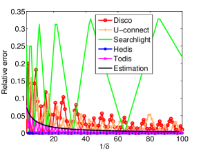
Figure 5: Relative error vs. small duty cycle $\delta$. The “Estimation" line is the theoretical upper bound estimation of relative error induced by Todis (see Section V).

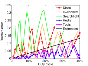
Figure 6: Relative error vs. large duty cycle $\delta$. The “Estimation" line is the theoretical upper bound estimation of relative error induced by Todis (see Section V).

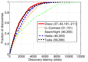
Figure 7: CDF of discovery latency when each pair of nodes operate at duty cycles $1\%$ and $5\%$, respectively. Numbers in the parentheses indicate the parameters of each corresponding protocol.

VI-A Duty Cycle Granularity

The first set of simulations comparatively studies the supported duty cycles. We study two groups of duty cycles:

1. Small duty cycles $1\leq 1/\delta\leq 100$, i.e., $\delta=1,\frac{1}{2},\frac{1}{3},\frac{1}{4},\ldots,\frac{1}{100}$;

2. Equispaced large duty cycles $0\leq\delta\leq 1$, i.e., $\delta=0\%,1\%,2\%,3\%,4\%,\ldots,100\%$.

We use the metric called the relative error (defined in Eq. 12) to quantify the capability of supporting each studied duty cycle, which is denoted as

$$\epsilon\triangleq|\delta^{\prime}-\delta|/\delta,$$

where $\delta^{\prime}$ is the closest duty cycle that is supported by each simulated protocol, w.r.t. $\delta$. Note that a smaller $\epsilon$ implies that the protocol provides more choices for energy conservation with a finer granularity of duty cycle control. For Searchlight, we let the smallest duty cycle unit be $1/2$ to allow the finest duty cycle granularity.

Figure 7 illustrates the results for small duty cycles, while Figure 7 shows those of large duty cycles. These results provide us the following insights:

• Searchlight is inferior to the other protocols in supporting various duty cycles because it requires the duty cycle to be $\frac{2}{t^{i}}$, where $t$ is a fixed integer and $i=1,2,3,\ldots$. In this simulation, we use $t=2$ to give Searchlight support for the duty cycles $1,\frac{1}{2},\frac{1}{4},\frac{1}{8},\ldots$. The relative error increases significantly as the desired duty cycle deviates away from the supported duty cycles (e.g., in Figure 7, it has a peak at $37.5\%=\frac{1/2+1/4}{2}$, and $1/2$ and $1/4$ are supported duty cycles).

• The schedules in Disco and U-Connect are generated using prime numbers, which have a denser distribution than power-multiples. Thus, Disco and U-Connect perform better than Searchlight.

• Both Hedis and Todis greatly outperform all the other protocols, having very small relative errors. In fact, for small duty cycles, the relative errors from Hedis is nearly constantly zero (see Figure 7). On the other hand, although Todis also performs well, its error rate obviously increases much faster than Hedis as the duty cycle $\delta$ increases.

• The theoretical “Estimation" lines for Todis (see Figures 7 and 7) holds up well in that it follows the same pattern as Todis’ actual error rates. This confirms our prior analysis in section V of Todis’ duty cycle granularity, where we estimated the upper bound relative error for Todis.

VI-B Discovery Latency

In this set of simulations, we study the discovery latencies of these protocols. For each simulation, we take 1000 independent pairs of nodes and assign various duty cycles. In two instances, we compare the protocols’ performance in heterogeneous discovery scenarios. We assign duty cycles of $1\%$ and $5\%$ to each respective node in the node pair in the first instance (see Figure 7), and $1\%$ and $10\%$ in the second instance (see Figure 10). We also compare the performance of the protocols in two homogeneous discovery scenarios, with each node in the node pair operating at the same duty cycles of $5\%$ in the first scenario (see Figure 10) and $1\%$ in the second one (see Figure 10).

Heterogeneous vs. homogeneous duty cycles. From these four cumulative distribution function graphs (CDFs), we see that overall, all of the protocols have comparative discovery latencies, with the odd exception of Searchlight in Figure 7. Nonetheless, it must be noted that all 5 protocols presented were eventually successful in neighbor discovery for $100\%$ of the pairs tested. These CDFs also show that Hedis is one of the few protocols that consistently perform above average in both the heterogenous and homogeneous neighbor discovery cases. For example, Figures 10 and 10 indicate that Searchlight is the clear winner for discovery latency in the homogeneous case, but it does poorly in the heterogeneous cases, as seen in Figures 7 and 10.

In addition, we see that for up to $90\%$ of the CDF, Hedis and Todis are both near top performers, but the protocol with one of the smallest latencies in reaching $100\%$ of the CDF in every case is U-Connect. We attribute this to the fact that U-Connect uses smaller values as its parameters, thus having a smaller upper bound in the worst case.

Similarly, we attribute Todis’ consistent long tail in each CDF scenario to its larger parameters. Therefore, although it can quickly allow nodes to discover each other in most cases, seen in its quickly reaching $90\%$ in the CDFs, it has the longest latency in the worst-case scenarios.

Hedis vs. Todis. These various simulations show that Hedis and Todis optimize the duty cycle granularity in both the quorum based and the co-primality based neighbor discovery approaches, with Hedis having a finer granularity than Todis. Additionally, both protocols perform reasonably well in terms of discovery latency, with Todis having a larger worst case latency bound due to its larger parameters.

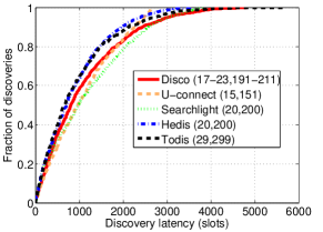
Figure 8: CDF of discovery latency when each pair of nodes operate at duty cycles $1\%$ and $10\%$, respectively. Numbers in the parentheses indicate the parameters of each corresponding protocol

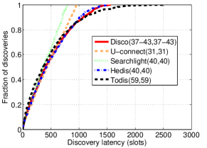
Figure 9: CDF of discovery latency when each pair of nodes operate at the same duty cycle of $5\%$. Numbers in the parentheses indicate the parameters of each corresponding protocol.

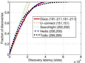
Figure 10: CDF of discovery latency when each pair of nodes operate at the same duty cycle of $1\%$. Numbers in the parentheses indicate the parameters of each corresponding protocol.

VII Conclusion

In this paper, we explored the current two main approaches of designing an asynchronous heterogeneous neighbor discovery protocol with guaranteed latency upper bounds—the quorum based and the co-primality based approaches. Using these two approaches we designed the Hedis and Todis neighbor discovery protocols, emphasizing on duty cycle granularity optimization for both. Hedis, as a quorum based protocol, forms a $(n-1)\times n$ matrix of time slots and uses the anchor- probing slot method to ensure neighbor discovery. Todis, as a co-primality based protocol, uses sets of three consecutive odd integers to ensure co-primality and thus ensures neighbor discovery due to CRT. In the design of both protocols we proved their capability in ensuring acceptable upper bounds in discovery latency. Through analytical comparisons as well as simulations, we confirmed the optimality of Hedis and Todis in duty cycle granularity among existing protocols. Hedis is able to support duty cycles in the form of $\frac{2}{n}$, while Todis can support duty cycles roughly in the form of $\frac{3}{n}$, allowing both protocols to effectively cover any practical duty cycle and thus prolong battery longevity.

We also showed in both our analysis and simulations that Hedis as a quorum based protocol is better than Todis as a co-primality based protocol in both duty cycle granularity and discovery latency, although differences by the latter metric are minor. By being able to support duty cycles at such a fine granularity while still guaranteeing an acceptable discovery latency bound, Hedis truly paves the way for neighbor discovery in wireless sensor networks.

References

- [1] G. Anastasi, M. Conti, M. Di Francesco, and A. Passarella. Energy conservation in wireless sensor networks: A survey. Ad Hoc Networks, 7(3):537–568, 2009.
- [2] M. Bakht, M. Trower, and R. H. Kravets. Searchlight: won’t you be my neighbor? In Proceedings of the 18th annual international conference on Mobile computing and networking, pages 185–196. ACM, 2012.
- [3] P. Dutta and D. Culler. Practical asynchronous neighbor discovery and rendezvous for mobile sensing applications. In Proceedings of the 6th ACM conference on Embedded network sensor systems, pages 71–84. ACM, 2008.
- [4] L. M. Feeney and M. Nilsson. Investigating the energy consumption of a wireless network interface in an ad hoc networking environment. In INFOCOM 2001. Twentieth Annual Joint Conference of the IEEE Computer and Communications Societies. Proceedings. IEEE, volume 3, pages 1548–1557. IEEE, 2001.
- [5] V. Galluzzi and T. Herman. Survey: discovery in wireless sensor networks. International Journal of Distributed Sensor Networks, 2012, 2012.
- [6] J.-R. Jiang, Y.-C. Tseng, C.-S. Hsu, and T.-H. Lai. Quorum-based asynchronous power-saving protocols for ieee 802.11 ad hoc networks. Mobile Networks and Applications, 10(1-2):169–181, 2005.
- [7] A. Kandhalu, K. Lakshmanan, and R. R. Rajkumar. U-connect: a low-latency energy-efficient asynchronous neighbor discovery protocol. In Proceedings of the 9th ACM/IEEE International Conference on Information Processing in Sensor Networks, pages 350–361. ACM, 2010.
- [8] S. Lai, B. Ravindran, and H. Cho. Heterogenous quorum-based wake-up scheduling in wireless sensor networks. Computers, IEEE Transactions on, 59(11):1562–1575, 2010.
- [9] M. J. McGlynn and S. A. Borbash. Birthday protocols for low energy deployment and flexible neighbor discovery in ad hoc wireless networks. In Proceedings of the 2nd ACM international symposium on Mobile ad hoc networking & computing, pages 137–145. ACM, 2001.
- [10] E. Miluzzo, N. D. Lane, K. Fodor, R. Peterson, H. Lu, M. Musolesi, S. B. Eisenman, X. Zheng, and A. T. Campbell. Sensing meets mobile social networks: The design, implementation and evaluation of the cenceme application. In Proceedings of the 6th ACM Conference on Embedded Network Sensor Systems, SenSys ’08, pages 337–350, New York, NY, USA, 2008. ACM.
- [11] M. B. Nathanson. Elementary methods in number theory, volume 195. Springer, 2000.
- [12] A.-K. Pietiläinen, E. Oliver, J. LeBrun, G. Varghese, and C. Diot. Mobiclique: Middleware for mobile social networking. In Proceedings of the 2Nd ACM Workshop on Online Social Networks, WOSN ’09, pages 49–54, New York, NY, USA, 2009. ACM.
- [13] Y.-C. Tseng, C.-S. Hsu, and T.-Y. Hsieh. Power-saving protocols for ieee 802.11-based multi-hop ad hoc networks. Computer Networks, 43(3):317–337, 2003.
- [14] S. Vasudevan, J. Kurose, and D. Towsley. On neighbor discovery in wireless networks with directional antennas. In INFOCOM 2005. 24th Annual Joint Conference of the IEEE Computer and Communications Societies. Proceedings IEEE, volume 4, pages 2502–2512 vol. 4, March 2005.
- [15] S. Vasudevan, D. Towsley, D. Goeckel, and R. Khalili. Neighbor discovery in wireless networks and the coupon collector’s problem. In Proceedings of the 15th Annual International Conference on Mobile Computing and Networking, MobiCom ’09, pages 181–192, New York, NY, USA, 2009. ACM.
- [16] W. Zeng, S. Vasudevan, X. Chen, B. Wang, A. Russell, and W. Wei. Neighbor discovery in wireless networks with multipacket reception. In Proceedings of the Twelfth ACM International Symposium on Mobile Ad Hoc Networking and Computing, MobiHoc ’11, pages 3:1–3:10, New York, NY, USA, 2011. ACM.
- [17] D. Zhang, T. He, Y. Liu, Y. Gu, F. Ye, R. K. Ganti, and H. Lei. Acc: Generic on-demand accelerations for neighbor discovery in mobile applications. In Proceedings of the 10th ACM Conference on Embedded Network Sensor Systems, SenSys ’12, pages 169–182, New York, NY, USA, 2012. ACM.
- [18] D. Zhang, T. He, F. Ye, R. Ganti, and H. Lei. Eqs: Neighbor discovery and rendezvous maintenance with extended quorum system for mobile sensing applications. In Distributed Computing Systems (ICDCS), 2012 IEEE 32nd International Conference on, pages 72–81, June 2012.
- [19] Z. Zhang and B. Li. Neighbor discovery in mobile ad hoc self-configuring networks with directional antennas: algorithms and comparisons. Wireless Communications, IEEE Transactions on, 7(5):1540–1549, May 2008.
- [20] R. Zheng, J. C. Hou, and L. Sha. Asynchronous wakeup for ad hoc networks. In Proceedings of the 4th ACM International Symposium on Mobile Ad Hoc Networking &Amp; Computing, MobiHoc ’03, pages 35–45, New York, NY, USA, 2003. ACM.