The analysis of realistic Stellar Gaia mock catalogues. I. Red Clump Stars as tracers of the central bar

Abstract

In this first paper we simulate the population of disc Red Clump stars to be observed by Gaia. We generate a set of test particles and we evolve it in a 3D barred Milky Way like galactic potential. We assign physical properties of the Red Clump trace population and a realistic 3D interstellar extinction model. We add Gaia observational constraints and an error model according to the pre-commissioning scientific performance assessments. We present and analyse two mock catalogues, offered to the community, that are an excellent test bed for testing tools being developed for the future scientific exploitation of Gaia data. The first catalogue contains stars up to Gaia G$\sim$20, while the second is the subset containing Gaia radial velocity data with a maximum error of $\sigma_{V_{r}}=10$km s^-1. Here we present first attempts to characterise the density structure of the Galactic bar in the Gaia space of observables. The Gaia large errors in parallax and the high interstellar extinction in the inner parts of the Galactic disc prevent us to model the bar overdensity. This result suggests the need to combine Gaia and IR data to undertake such studies. We find that IR photometric distances for this Gaia sample allow us to recover the Galactic bar orientation angle with an accuracy of $\sim 5^{\circ}$.

1 Introduction

Special emphasis has been put recently on characterising the Galactic disc and its non-axisymmetric structures. Upcoming big surveys, such as Gaia (ESA), will provide us with the opportunity to increase the extent of the region with detailed kinematic information from few hundreds of parsecs to few kiloparsecs and with unprecedented precision. This larger volume of study makes it reasonable to question whether Gaia will be able to characterise the Galactic bar and the spiral arms, both in density, by determining overdensities, and in kinematics, by analysing the imprints that these structures leave in the velocity space (e.g. Dehnen, 2000; Fux, 2001; Gardner & Flynn, 2010; Minchev et al. , 2010; Antoja et al. , 2011) . One of the regions of great interest in the galactic disc is the end of the bar region. It can provide information regarding the link between the spiral arms and the bar. Besides, this is a possible line-of-sight to be observed by the Gaia-ESO Survey.

In this paper we provide mock catalogues which are a suitable test bed for such studies. Several analysis have already started using these catalogues, for example the use of the vertex deviation to determine the resonant radii of galaxy discs (Roca-Fabrega et al. , 2014), or determining the tilt and twist angles of the Galactic warp (Abedi et al. , 2014). Single population catalogues generated using test particle simulations together with a realistic extinction map, as proposed here, have demonstrated to be well suited to perform these kind of studies. The advantage of using test particles evolved in a realistic galactic potential, instead of samples generated from at present Galaxy models (e.g. the Besançon Galaxy Model (Czekaj et al. , 2014)), is that the stars have been evolved according to a known galactic potential and have inherited the information on both density and kinematics, that is the stars are in statistical equilibrium with the potential imposed. With respect to N-body simulations, the advantages are that we control the potential used and that we can choose the parameters of the potential to resemble that of the Milky Way. Thus, by changing the parameters of the potential, such as disc mass, bar length, bar pattern speed, we obtain new mock catalogues fulfilling the new kinematic imprints of the mass model imposed. This fact allows us to consider the inverse problem once we have the Gaia data. That is, determining the free parameters of the potential whose characteristics match the observed data.

Here we present two mock catalogues of Red Clump stars with the set of observables that Gaia will provide. The first contains all such disc stars up to Gaia G magnitude of $20$, for which Gaia will provide astrometric and photometric data. The second catalogue is the subset containing also Gaia radial velocity data. This reduces the sample to stars up to magnitude G approximately $16$. The potential used to generate the catalogues is 3D, with a rotation curve that matches that of the Milky Way and it includes the expected non-axisymmetric structure, i.e. the Galactic bar. During the integration, response spiral arms arise. However, we will not discuss them in this paper. The number of particles has been set to match the local surface density of the Red Clump population.

It has been long established that the Red Clump K-giants (hereafter, RC) are a good tracer population suitable to study the Galactic structure. First, RC stars are abundant enough and sufficiently bright (Paczynski & Stanek, 1998; Stanek & Garnavich, 1998; Zasowski et al. , 2013). Second, theoretical models predict that RC stars absolute luminosity barely depends on their age and chemical composition. RC stars have been used in various studies of the Galactic disc, for example to estimate the distance to the Galactic centre (Paczynski & Stanek, 1998), to propose the presence of a Long bar (López-Corredoira et al. , 2007), or for the analysis of streaming motions in the disc (Williams et al. , 2013). Gaia works in the optical range of spectra, with the known limitation of not reaching deeply in the galactic disc. Furthermore, Gaia’s spectrograph is not able to provide radial velocities for the faintest stars. Undergoing surveys in the infra-red, therefore, become necessary to complement Gaia data, e.g. APOGEE (Apache Point Observatory Galactic Evolution Experiment) (Eisenstein et al. , 2011), from which accurate radial velocities are measured, and precise distances to the RC stars are provided (Bovy et al. , 2014). The authors select the RC stars from the APOGEE survey based on their position in colour-metallicity-surface-gravity-effective-temperature space using a new method calibrated using stellar-evolution models and high-quality asteroseismology data. The particular narrow position of the RC stars in the colour-metallicity-luminosity space allows the authors to assign distances to the stars with a precision of $5$ to $10\%$, which is better than the Gaia precision far from the Solar neighbourhood (see Sect. 3.2). In this work, therefore, we also consider observed distances with IR errors, instead of parallax errors.

By either using the astrometric, photometric and spectroscopic error models defined by the Gaia mission before commissioning or relative distance errors provided by photometric distances, we convolve our model stars into observables. The mock catalogues presented here can be easily readjusted to future error models after commissioning, or first and second data releases.

As a first exploitation of these mock catalogues, we study whether Gaia will be able to detect and characterise the Galactic bar, by either directly detecting its overdensity, or by analysing its imprint in the kinematic space (Romero-Gómez et al, in preparation). Regarding the bar overdensity, recent papers (Martinez-Valpuesta & Gerhard, 2011; Romero-Gómez et al. , 2011) rise the possibility that only one long boxy-bulge bar is present in the Milky Way, contrary to what other studies suggest (Hammersley et al. , 2000; Benjamin et al. , 2005; López-Corredoira et al. , 2007), namely a triaxial bulge plus a misaligned long bar. Will Gaia be able to determine the bar characteristics? Although we know that Gaia data will not reach the Bulge region, we will extend our study from the Solar Neighbourhood to a spherical region of about $4-5$kpc, to which we refer as the Gaia sphere. Can Gaia detect the dynamical effects of the bar(s) in the Gaia sphere?

This paper is organized as follows. First, in Sect. 2 we describe our 3D test particle simulation, namely the initial conditions, the gravitational potential model, the integration process and the construction of the two mock catalogues. In Sect. 3, we analyse the surface density, the distribution of the parallax accuracies and the distribution of the radial and tangential velocities accuracies of the catalogues. Then, in Sect. 4 we present the characterisation of the Galactic bar in the space of observables and the Gaia possibilities to detect it, suggesting a necessary link with IR surveys. Finally, our conclusions are presented in Sect. 5.

2 The simulations

Most of the previous studies using test particle simulations with a bar potential were 2D and focused on the kinematics of regions near the Sun (e.g. Dehnen 2000; Fux 2001; Gardner & Flynn 2010; Minchev et al. 2010; Antoja et al. 2011). Only recent papers, such as Monari et al. (2014) start using 3D test particle simulations with similar goals as ours, this is, we want to model the signatures of the Galactic bar at large distances from the Sun. Our simulation aims to mimic the present spatial and kinematic distribution of the disc RC population in 3D and over a wide region of the Galaxy.

The total galactic potential consists of an axisymmetric component plus a bar-like potential. We choose the Allen & Santillán (1991) potential for the axisymmetric component, which consists of the superposition of a Miyamoto-Nagai disc, a spherical bulge and a spherical halo. The free parameters of the axisymmetric potential are chosen so that the rotation curves matches that of the Milky Way (Allen & Santillán, 1991).

In Sect. 2.1, we describe the initial conditions, while in Sect. 2.2 we give the details of the 3D galactic barred model considered. In Sect. 2.3, we describe the integration process. Finally, in Sect. 2.4, we assign the physical properties of the RC population and Gaia errors.

2.1 Setting up the initial conditions

The initial conditions follow the density distribution of the Miyamoto- Nagai disc (Miyamoto & Nagai, 1975) with the parameters set in Allen & Santillán (1991). They are generated using the Hernquist method (, 1993). The velocity field is approximated by gaussians, whose parameters are obtained from the first order moments of the collisionless Boltzmann equation, simplified by the epicyclic approximation. The details are shown in the Appendix A of the paper.

We consider a single population with the characteristics of the RC K-giants. That is, we fix the velocity dispersions at the Sun position to be $\sigma_{U}=30.3$km s^-1, $\sigma_{V}=23.6$km s^-1and $\sigma_{W}=16.6$km s^-1(Binney & Tremaine, 2008, and references therein), and a constant scale-height of $300$pc (Robin & Creze, 1986). The asymmetric drift has been taken into account when computing the tangential component of the velocity.

As previously mentioned, the number of particles in the disc has been set to match the surface density of RC stars in a local neighbourhood. We consider a cylinder for all $z$ of radius $100$pc centred in the Solar position and by using the new Besançon Galaxy Model (Czekaj et al. , 2014), we obtain a surface density of stars of $0.05614$stars/pc² (Czekaj, private communication). This surface density is imposed to the set of test particlesobtained after relaxation (see Sect. 2.3). The suitable amount of disc RC stars that matches this surface density is $57\times 10^{6}$, and this is the number of particles we will use in our simulations.

As in Allen & Santillán (1991), we assume the Sun is located at $R_{\odot}=8.5$kpc, the local standard of rest rotates with a circular velocity of $V_{c}(R_{\odot})=220$km s^-1and the Sun peculiar velocity is $(U,V,W)_{\odot}=(10.,5.25,7.17)$km s^-1(Dehnen & Binney, 1998). Throughout the paper, the Galactic Centre is located in the origin of coordinates and the Sun is located on the negative x-axis.

2.2 The bar model

We aim to model the Galactic bar as a bar with a boxy/bulge, i.e. the COBE/DIRBE triaxial bulge, plus the long bar. For this, we use a simple model which consists of the superposition of two Ferrers ellipsoids (Ferrers, 1877) with non-homogeneity index equal to $n=1$ (Romero-Gómez et al. , 2011; Martinez-Valpuesta & Gerhard, 2011). The main parameters of the models are fixed to values within observational ranges (see Romero-Gómez et al. (2011)). For the COBE/DIRBE bulge we set the semi-major axis to $a=3.13$kpc and the axes ratios to $b/a=0.4$ and $c/a=0.29$. The mass is $M_{CB}=4.5\times\,10^{9}$M_⊙. The length of the Long bar is set to $a=4.5$kpc and the axes ratios to $b/a=0.15$ and $c/a=0.026$. The mass of the long bar is fixed to $M_{LB}=2.5\times\,10^{9}$ M_⊙. So finally we obtain a boxy/bulge type of bar with total mass equal to $M_{b}=7.\times 10^{9}$M_⊙. Both major axes are aligned on the x-axis of the rotating reference system and we will refer to the superposition of these two ellipsoids as the Galactic bar.

The Galactic bar is oriented at $20^{\circ}$ from the Sun-Galactic Centre line. It rotates at a constant angular speed of $50$km s^-1 kpc^-1around the short z-axis. This value is within the range accepted for the COBE/DIRBE bar of the Milky Way (Gerhard, 2011).

2.3 The integration process

We obtain the final mock catalogue following three steps. We first integrate the disc initial conditions in the axisymmetric Allen & Santillán (1991) potential alone, to allow particles to reach a reasonable state of statistical equilibrium with the total axisymmetric component. After some trial and error, and being conservative, we opted for an integration time of $10\,Gyr$.

Secondly, the non-axisymmetric component is introduced adiabatically in four bar rotations ($T_{grow}\sim 500\,Myr$). During this time, we require that the total mass of the system ($9\times 10^{11}\,M_{\odot}$) remains constant. To do this we consider a progressive mass transfer from the initial spherical bulge of the Allen & Santillán model to the bar in the following way:

$$\Phi_{T}(x,y,z,t)=\Phi_{d}+\Phi_{h}+(1-f(t)f_{0})\Phi_{bul}+f(t)\Phi_{b},$$

where $\Phi_{T}$ denotes the total potential. $\Phi_{d}$, $\Phi_{h}$ and $\Phi_{bul}$ are the disc, halo and bulge axisymmetric components of the Allen & Santillán (1991) potential, respectively, and $\Phi_{b}$ denotes the bar potential. For the time function $f(t)$ we adopt the same fifth degree polynomial of time, $t$, as in Eq.(4) of Dehnen (2000). It has continuous derivatives guaranteeing a smooth transition from the non-barred to the barred state. $f_{0}$ is defined as $f_{0}=M_{b}/M_{bul}$. Therefore, when $t=T_{grow}$, we have a bar of $M_{b}=7.\times 10^{9}$M_⊙ and a residual axisymmetric bulge of mass $M_{bul}=7.\times 10^{9}$M_⊙. Therefore, in the central part of the Galaxy there is a boxy/bulge type of bar plus an axisymmetric bulge with a total mass $1.4\times 10^{10}$M_⊙.

Finally, once the bar has been introduced, we integrate the particles in the total potential for another four bar rotations, again to allow the particles to reach a reasonable state of statistical equilibrium now with the final potential. In the following sections, we will analyse, the RC population in this final snapshot. We name this whole particle set as RC-all. We want to stress that the samples presented here are not a self-consistent dynamical solution, but rather a tracer population that has reached, to a large extent and by construction, statistical equilibrium with the final assumed potential.

We show in Fig. 1 the surface density map corresponding to the RC-all sample. In this and following plots we divide the sample in galactocentric cylindrical bins $(R,\theta)$ of size $100$pc $\times 0.72^{\circ}$, where $R\in[0,10]$kpc and $\theta\in[0,360^{\circ}]\,$. In the case of Fig. 1, we can clearly see the central non-axisymmetric component, i.e. the bar, in the surface density.

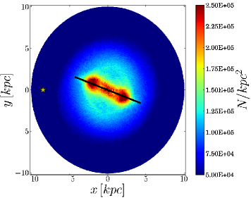
Figure 1: Surface density (Number of stars / $kpc^{2}$) in each of the regions of the full sample model (RC-all). The yellow star shows the Sun position and the black solid line marks the position of the bar.

2.4 The RC physical parameters assignment

The derivation of the Gaia G magnitude and the computation of the Gaia astrometric, photometric and spectrophotometric standard errors for the RC stars are calculated following the strategy outlined in the Gaia (ESA) webpage. This page is regularly updated according to the scientific performance assessments for Gaia during mission operation. The pre-launch performance models have been used in this paper. New prescriptions proposed after the commissioning phase (ended July 2014) have been recently published and more changes are expected before the first Gaia Data Release (mid 2016). These changes will be regularly applied to the catalogues presented here.

Our test particles are characterised as Red Clump K-giant stars, that is K0-1 III stars. Here we assume they have an absolute magnitude of $M_{K}=-1.61$ (Alves, 2000) without intrinsic dispersion in brightness and intrinsic colors of $(V-I)_{o}=1.0$ and $(V-K)_{o}=2.34$ (Alves, 2000). From the previous section, we have assigned a galactocentric position to each star, which we can transform to heliocentric coordinates $(d,l,b)$, where $d$ is the heliocentric distance in kpc and $(l,b)$ are the galactic longitude and latitude, respectively. The 3D extinction model of Drimmel, Cabrera-Lavers & López-Corredoira (2003) using scaling factors has been used to assign a visual absorption $A_{V}$ to the stars. The authors compute the scaling factors to correct the dust column density of the smooth model to account for small scale structure of the dust and gas not considered in the model. They are direction dependent factors based on the FIR residuals between the DIRBE 240$\mu m$ data and the predicted emission of the parametric dust distribution model. We assume then the extinction law from Cardelli, Clayton & Mathis (1989) ($A_{K}=0.114A_{V}$ and $A_{I}=0.479A_{V}$) to finally compute the apparent magnitude in V and the observed (V-I) colour index. The Gaia magnitude, G, and the $(B_{p}-R_{p})$ colours are computed from a third degree polynomial fit depending on the apparent magnitude V and the (V-I) colour (see Table 3 of (2010)).

The end-of-mission errors in astrometry depend on the magnitude G of the star and its observed (V-I) colour (see Gaia Science Performance webpage mentioned above). They also vary over the sky as a result of the scanning law due to the different number of transits at the end of the mission (see Table 6 in the Gaia Science Performance webpage). Radial velocities will be obtained for stars brighter than $V\sim 17$ mag through Doppler-shift measurements by the Radial Velocity Spectrometer (RVS).

3 The RC mock catalogues

Once we have assigned the physical parameters of the RC stars to the simulated test particles, we obtain two simulated catalogues from our full disc simulation (RC-all). Both catalogues include the effects of the absorption computed using the 3D Drimmel extinction model with scaling factors mentioned above.

The first catalogue, namely the RC-G20 sample, contains all stars with magnitude $G\leq 20$, as this is the limiting magnitude for Gaia astrometric and spectrophotometric data. The second catalogue, called RC-RVS, contains only stars having a radial velocity error $\sigma_{V_{r}}\leq 10$km s^-1. According to the Gaia Science Performance, the model for the radial velocity errors is valid for stars with $G_{rvs}\leq 16.1$, and the analytical expression for the error is an exponential function that depends on the magnitude V of the star and its spectral type. We add the Gaia errors to the astrometric and photometric variables and to the radial velocities of both samples, obtaining the observed mock catalogues, RC-G20-O and RC-RVS-O, respectively, where O stands for observed. In Table 1, we summarize the total number of stars of the samples considered. Cutting the RC-all sample to the stars that Gaia will see means reducing the total number of particles by a half. Furthermore, considering a sample with good radial velocities, RC-RVS, reduces the number of particles in the sample by a factor of 7.

Figure. 2 shows the histograms in the magnitude $G$ for the RC-G20 sample (red) and for the RC-RVS sample (blue). The latter, which is obviously included in RC-G20, shows a limiting magnitude $G$ of about 16 mag, which is the result of the cut in radial velocity error of $\sigma_{V_{r}}\leq 10$km s^-1. The flattening in the number of particles at faint magnitudes in the RC-G20 sample is due to the combination of two facts: the effect of the spatial density distribution and the high interstellar extinction at large distances in the plane.

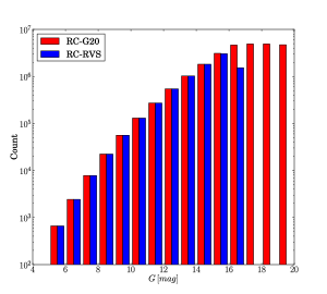
Figure 2: Histograms in logscale of the magnitude $G$ for the RC-G20 (red) and RC-RVS (blue) samples.

	Number of stars
RC-all	$57\times 10^{6}$
RC-G20	$26\times 10^{6}$
RC-RVS	$8.5\times 10^{6}$

Table 1: Total number of stars of the samples used in the paper, namely RC-all with all the particles in the disc, RC-G20 with all the particles with Gaia G magnitude up to 20 mag and RC-RVS with all the particles with radial velocity error $\sigma_{V_{r}}\leq 10$km s^-1.

However, as discussed further in Sect. 4.2, one of the advantages of using the RC population is that we can complement the Gaia data with other ongoing IR surveys, such as APOGEE or UKIDSS. As previously mentioned, distances derived from photometry will be more precise than trigonometric parallaxes for stars far from the Gaia sphere. Bovy et al. (2014) derived spectro-photometric distances using high-resolution spectroscopic APOGEE data and NIR and mid-IR photometry. The authors estimated that distances for RC stars can be derived with an accuracy of $5$ to $10\%$. At present, the APOGEE survey covers only specific regions in the sky so this data would not be available for the full sky Gaia data. Photometric distances computed using only IR photometry will be needed (e.g. Cabrera-Lavers et al. , 2007). This second strategy suffers from contamination from non-RC stars, which would degrade distance estimation introducing some systematic trends. Recently, López-Corredoira et al. (2014) reported that for faint stars, the contamination due to non-RC stars could reach $20\%$. On the other hand, using 2MASS photometry and assuming an intrinsic dispersion of $\sigma_{K}=0.22$ for RC stars (Alves, 2000), by error propagation of the distance modulus, $M_{K}=m-5\log 10(d)+5-A_{K}$, a relative error in distance of about $10\%$ is estimated (Monari et al. , 2014). Taking into account all these considerations, a relative error in distance of $10\%$ seems reasonable and it will be assumed here for our RC IR-distances. Therefore, in RC-G20-IR we convolve the RC-G20 mock catalogue with IR photometric distances.

3.1 The RC surface density

In Figure 3 we show the surface density of the RC-G20 and the RC-RVS samples. This gives us an estimation of the number of RC stars that we can expect in the Gaia catalogue in different locations in the disc. Here the stars are distributed using their real distances, i.e. not affected by errors. The surface density looks different in each sample since both samples have a different magnitude cut. Taking into account all these facts, Gaia will be able to provide proper motions for the RC stars located at the end of the bar with the RC-G20 sample but not radial velocities (left panel). However, as expected, the number of particles in this region decreases when we require the particles to have good radial velocities, that is for the RC-RVS sample (right panel).

In the bottom panels of Fig. 3, we show the distribution of stars in $(x,z)$ plane coloured according to the absorption in V, $A_{V}$. As expected, particles closer to the Galactic plane have higher absorption. In both cases, a $65\%$ of the particles in the sample lie within $|z|<300$pc.

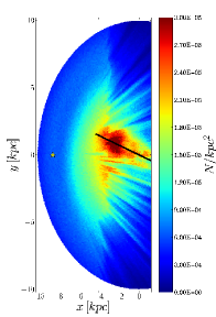
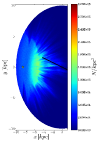
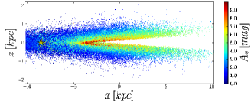
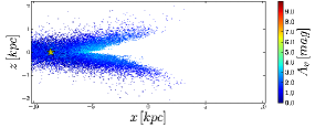
Figure 3: The RC-G20 and RC-RVS samples. First row: As in Fig. 1 for the RC-G20 and RC-RVS samples, respectively. Note that the stars are distributed using their real distances, i.e. not affected by errors. The yellow star in both panels shows the position of the Sun and the black solid line marks the position and length of the bar. Second row: $(x,z)$ projection, the colour indicates the absorption in V given by the Drimmel, Cabrera-Lavers & López-Corredoira (2003) model.

3.2 Parallax precision distribution

In this section we study the mean relative error in parallax in the RC-G20 and RC-RVS samples. In the following plots, we show only the near side of the Galaxy, that is $x<1$kpc. Due to extinction effects, the vertical distribution of the particles inside a cylinder perpendicular to the plane is not maintained for a given line-of-sight, therefore, in Fig. 4 we divide each sample in two, namely particles closer to the Galactic plane with $|z|<300$pc (top), and particles less affected by the extinction, this is, particles such that $|z|>300$pc (bottom). As expected, the distribution of the mean relative errors in parallax changes through the Galactic plane when we compare the RC-G20 (left) and RC-RVS samples (right). For a fixed position in the disc, requiring a sample with good radial velocities translates into a sample with less number of particles more distributed above the plane as seen in the bottom right panel of Fig. 3. When we compare the samples with particles closer to the galactic plane (top panels) we see that the RC-RVS sample reaches a given mean relative error in parallax at larger distance than the RC-G20 sample. This is because, at this distance, the stars that remain in the RC-RVS sample are in mean brighter than the corresponding RC-G20 sample. As a consequence, the mean relative error in parallax at this point is smaller. At the same heliocentric distance, the RC-G20 sample is fainter in mean and, therefore, the mean relative error in parallax is larger. The same argument holds when we compare the sample for stars located at $|z|>300\,pc$, so less affected by extinction (bottom panels). At the same heliocentric distance the number of stars per bin of the RC-RVS sample is significantly less and only the bright stars contribute to the mean, thus, it has smaller mean relative error in parallax.

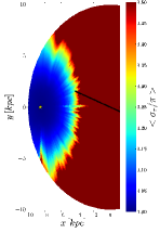
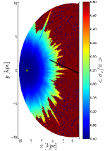
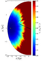
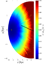
Figure 4: The mean relative error in parallax for the RC-G20 (left) and RC-RVS (right) samples for stars closer to the Galactic plane, $|z|<300\,pc$ (top) and beyond $|z|>300\,pc$ (bottom). Note that the stars are distributed using their real distances, i.e. not affected by errors. The yellow star in all panels shows the position of the Sun, while the black solid line marks the position and length of the bar.

The relative error in parallax for the particular case of the Sun-Galactic Centre line is shown in Fig. 5 for the RC-G20 sample. Each curve represents the number of stars per $kpc^{2}$ as a function of the relative error in parallax for the particles located in the Sun - Galactic Centre line. Each colour corresponds to particles that are located at a certain distance from the Sun projected on the x-axis, $d_{x}$, before introducing Gaia errors. As expected, particles located close to the Sun’s position have smaller errors, while the number of particles with higher errors increases as we move away from it. Also note that $95\%$ of the RC stars in this line-of-sight will have a relative error in parallax less than $20\%$ and we will have particles with this relative parallax error up to $5\,kpc$ from the Sun (yellow line). The relative error in parallax for four specific low extinction lines below the Galactic plane, including the Baade’s window, are shown in Fig. 11 in Sect. 3.5.

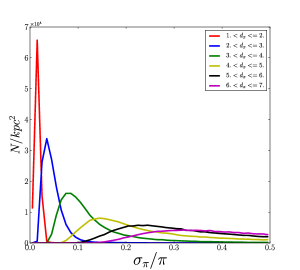
Figure 5: Histograms of the relative error in parallax as a function of the distance along the Sun - Galactic Centre line for the RC-G20 sample.

The distribution of errors in parallax shown in Fig. 4 translates in a redistribution of the particles when we add the Gaia errors. In Figure 6, we plot the surface density of the RC-G20-O (left) and RC-RVS-O (right) using the observed distances. The overdensity due to the bar is blurred and an accumulation of the particles takes places towards the Sun so that the central longitudes look more dense. Furthermore, we have to take into account that distances are biased when derived from the observed parallaxes. Since their relation is non-linear, the value $1/\pi_{obs}$ is a biased estimate of the true distance (Brown, Arenou, van Leeuwen et al. , 1997). The authors propose several methods to use astrometric data with minimal biases, such as using stars with the best relative errors, $\sigma_{\pi_{obs}}/\pi_{obs}<10\%$, though some biases due to the truncation are still expected, or other methods using all available information, though they are model dependent (Brown, Arenou, van Leeuwen et al. , 1997, and references therein). As discussed in Sect. 4.1, one of the suggestions in this work is working directly in the space of observables of the catalogue, here, the parallaxes.

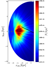
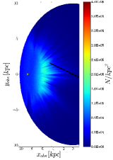
Figure 6: As in Fig. 3 for the samples RC-G20-O (left panel) and RC-RVS-O (right panel). The stars are distributed using their observed distances, i.e. affected by errors. The colour bar is different for each sample. The yellow star in both panels shows the position of the Sun. The solid black line shows the position and length of the bar.

The sky-averaged positions and proper motion relative errors distributions will follow the same pattern as the mean relative error in parallax presented here. As discussed in the Gaia Science Performance webpage, direct relations can be used, derived from scanning-law simulations.

3.3 Tangential and radial velocities precision distribution

In this section, we perform a similar analysis of the errors as in Sect. 3.2. We compute the mean error in tangential velocity for both samples, RC-G20 and RC-RVS and for two subsamples, namely one with stars above and below $|z|=300$pc, as in Sect. 3.2. For RC-RVS, we also compute the mean error in radial velocity. It is essential to know how the errors are distributed if we are interested in specific science projects, such as analysing the moments of the velocity distribution function (Romero-Gómez et al, in preparation).

We compute the mean error in tangential velocity on the plane in the sky, i.e. $V_{t}=k\mu d$, where $\mu$ is the proper motion defined as $\mu^{2}=\mu_{\alpha^{*}}^{2}+\mu_{\delta}^{2}$, and $\mu_{\alpha^{*}}=\mu_{\alpha}\cdot\cos(\delta)$ and $\mu_{\delta}$ are the proper motions in the right ascension and declination, respectively. $d$ is the heliocentric distance to the star and $k=4.74\frac{km/s}{``\,yr^{-1}pc}$ for the unit conversion. To compute the error in tangential velocity, we use, according to the Gaia Science Performance webpage, that the mean end-of-mission error in proper motion is $\sigma_{\mu}=0.526\sigma_{\pi}$, that the error in heliocentric distance is $\sigma_{d}=\sigma_{\pi}/\pi^{2}$. Both errors are taken into account to derive the error in the tangential velocity, $\sigma_{V_{t}}$. In the left panels of Fig. 7, we plot the mean error in tangential velocity for the particles in the RC-G20 assuming real distances and for the two subsamples above and below $|z|=300$pc.

This plot suggests that if we want a sample with maximum mean tangential velocity error of, for example, $10$km s^-1, the sample will reach up to $3.5$kpc from the Sun with stars closer to the Galactic plane and they will reach up to $4.5$kpc for stars above $|z|>300$pc, approximately in any direction. If we use IR photometric distances, the coverage increases up to half of the Galactic bar region in all heights (see right panels of Fig. 7). As expected, the errors in the end of the bar region are much lower when we use IR photometric distances than astrometric parallaxes. This justifies the need of IR surveys in the case we want to reach deeper in the disc.

In Fig. 8, we compute the histograms of the error in tangential velocity as a function of the distance projected on the x-axis to the Galactic Centre in the Sun - Galactic Centre line for the RC-G20 sample. Note how we will be able to have most of the stars with errors less than $10$km s^-1up to $5$kpc from the Sun.

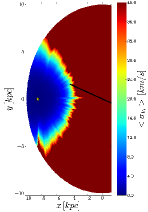
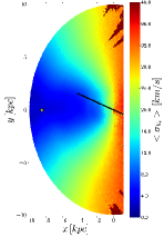
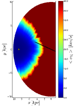
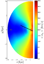
Figure 7: Mean errors in tangential velocity. Left panels, for the RC-G20 sample, that is, using the Gaia error model, and the stars distributed using the real distances. Right panels, mean errors in tangential velocity for the RC-G20-IR sample, that is, estimating the relative error in the distance to be constant and of $10\%$, which would correspond if the distances were obtained from the IR photometry. Top panels, for stars closer to the Galactic plane $|z|<300$pc. Bottom panels, for stars above $|z|>300$pc. The yellow star in both panels shows the position of the Sun.

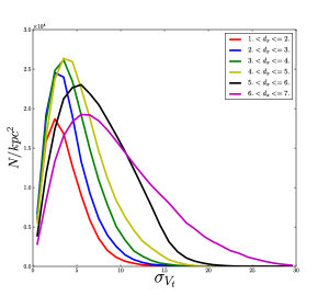
Figure 8: Histograms of the error in tangential velocity as a function of the distance along the Sun - Galactic Centre line for the RC-G20 sample.

In Fig. 9, we plot the mean errors in tangential velocity, again using both Gaia and photometric distance errors, and the mean errors in radial velocity for the RC-RVS sample and we divide again the sample in the particles below $|z|<300$pc (top panels) and above $|z|>300$pc (bottom panels). There is a big region, which is larger if the stars are outside the Galactic plane, for which the mean errors in tangential velocity obtained using Gaia, which includes the end of the bar region, are less than $15$km s^-1. But this region increases including almost half of the bar region, when using photometric distances. The mean errors in radial velocity in the bar region and outside the Galactic plane are in the range $4-6$km s^-1, while within the Gaia sphere the error is less than $4$km s^-1, for all heights.

In Table 2, we give the mean errors in two specific polar regions of $1\,kpc\times 10^{\circ}$, namely the regions near the end of the Long bar (hereafter LB region) and the end of the Boxy/bulge bar (hereafter BB region), for both the RC-G20 and RC-RVS samples and the two cuts in height. The galactocentric cylindrical coordinates of these points are given in the caption of Table 2. Note that the mean error in tangential velocity can be reduced by a factor 5 in some of these regions in the disc when using the IR photometric distances.

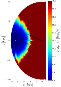
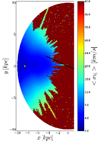
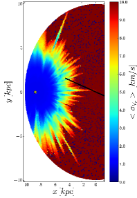
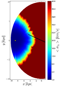
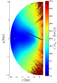
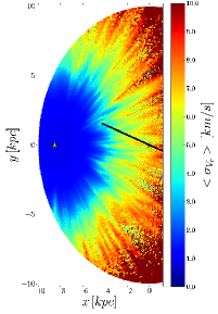
Figure 9: Mean errors in tangential and radial velocity in the RC-RVS sample. The stars are distributed using the real distances in the regions. Left and middle: Mean errors in tangential velocity using the Gaia error model and the IR photometric distance, respectively. Right: Mean errors in radial velocity. Top panels: for the subsample containing stars below $|z|<300$pc. Bottom panels: for the subsample containing stars above $|z|>300$pc. The yellow star in all panels shows the position of the Sun.

BB region
	RC-G20		RC-RVS
	$|z|<0.3$	$|z|>0.3$	$|z|<0.3$	$|z|>0.3$
$<\sigma_{V_{t}}>(Gaia)$	$>50$	25.8	24.9	20.9
$<\sigma_{V_{t}}>(IR)$	8.6	9.2	8.4	9.1
$<\sigma_{V_{r}}>$	—	—	9.5	5.0
LB region
	RC-G20		RC-RVS
	$|z|<0.3$	$|z|>0.3$	$|z|<0.3$	$|z|>0.3$
$<\sigma_{V_{t}}>(Gaia)$	19.6	11.5	12.8	11.4
$<\sigma_{V_{t}}>(IR)$	6.7	7.1	6.8	7.1
$<\sigma_{V_{r}}>$	—	—	6.3	4.4

Table 2: Mean errors in tangential and radial velocity for the RC-G20 and RC-RVS sample in the BB and LB regions and for different cuts in height. The region corresponding to LB is $(R,\theta)=(4.5kpc,160^{\circ})$, and the one corresponding to BB is $(R,\theta)=(3.1kpc,160^{\circ})$. The azimuthal angle is defined positively in the counter-clockwise direction from the x-positive axis. Units are kpc and km s^-1.

3.4 The vertical distribution at the near end of the bar

In this section we focus on the vertical distribution of stars in the BB and LB regions, that is, the two regions near the end of the Boxy/bulge and Long bar, respectively.

Figure 10 shows how the particles in the BB (top) and LB (bottom) regions are distributed in $|z|$ for the RC-G20, RC-G20-O, RC-RVS and RC-RVS-O. When we consider the RC-G20 sample without Gaia errors (blue lines), the number of particles changes depending on the position in the galactic disc. In the LB region, the number of particles decreases with height. However, in the BB region, the extinction increases and the number of particles decreases close to the galactic plane, until about $100$pc, where again the number of particles decreases with height. The effect of the Gaia errors depends again on the region. In the BB region, the amount of particles close to the galactic plane is much less, until about $100$pc, while for the LB region, we lose particles in the first $100$pc, but there are more near $200$pc. This redistribution of particles in height is basically an effect of the distance error (see Fig. 6).

The difference between the RC-RVS sample (green) and the RC-RVS-O sample (black) is not so evident, because requiring a high quality sample in terms of radial velocities also translates into a high quality sample in terms of parallaxes, as seen in Fig. 4. Therefore, the positions are not so affected by errors. There are no particles in the Galactic plane neither in the BB or LB regions. However, the number of particles increases up to $200\,pc$ in the case of the LB region, while in the BB region, there is still almost no particle at this height.

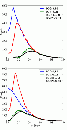
Figure 10: The vertical distribution of stars in the BB (top panel) and LB (bottom panel) regions for the RC-G20 (blue), RC-G20-O (red), RC-RVS (green) and RC-RVS-O (black) samples.

3.5 Below the Galactic Plane

Other interesting regions in the Galactic disc are the ones in the Bulge regions below the Galactic plane. These fields are interesting for the lower extinction and because spectroscopic data is being obtained by the BRAVA survey. In Fig. 11, we plot for both RC-G20 (left panels) and RC-RVS (right panels), information regarding four of the fields in the $l=0$ line-of-sight, namely $b=-2,\,-4,\,-6,\,-8^{\circ}$, as a function of the heliocentric distance, binned every $1$kpc. From top to bottom, we plot the histogram of the number of particles, the mean relative error in parallax, the mean error in tangential velocity, and the mean error in radial velocity. The number of RC stars detected by Gaia can complement the number of M giants in the BRAVA fields. As expected, the number of particles decrease when decreasing the galactic latitude, and when $b=-8^{\circ}$, the samples almost run out of particles. Due to the configuration of the ellipsoid bars imposed (see Fig. 12), at an heliocentric distance of $6\,kpc$ we reach the Galactic bar at $l=0$. For the RC-G20 sample, the mean relative error in parallax will be of $20-30\%$ at $b=-2^{\circ}$, for stars with an heliocentric distance of $6\,kpc$, and even less far below the plane. The mean error in tangential velocity is about $5$km s^-1in all the latitude bins at $6\,kpc$.

If we analyse the sample with good radial velocities, RC-RVS (right column of Fig. 11), we observe that for the fields closer to the Galactic plane ($b=-2,-4$), the sample runs out of particles at about $6$kpc, due to the imposed extinction law, while for $b=-6$ the density is approximately constant, but for $b=-8$ it decreases again. The mean relative error in parallax and the mean error in velocity improves with respect to the RC-G20 sample. Using the pre-commissioning error model for the radial velocity error, we obtain mean errors in radial velocities of maximum $5$km s^-1, that is, improving the errors given in the BRAVA surveys for this field (about $10$km s^-1) (Rich et al. , 2007; Kunder et al. , 2012).

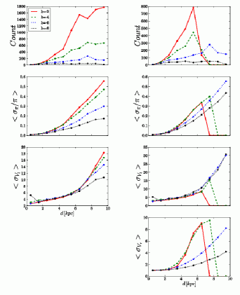
Figure 11: Number of particles and errors as a function of real heliocentric distance in four BRAVA fields along the $l=0$ line-of-sight, namely $b=-2$ (red solid line), $b=-4^{\circ}$ (green dashed line), $b=-6^{\circ}$ (blue dot-dashed line) and $b=-8^{\circ}$ (black dotted line) for the RC-G20 sample (left column) and RC-RVS sample (right column). First row: histogram of the number of particles. Second row: mean relative errors in parallax. Third row: mean errors in tangential velocity (units: km s^-1). Fourth row: mean errors in radial velocity (units: km s^-1). We do not plot the mean errors in radial velocities for the RC-G20 sample because not all particles will have valid radial velocities.

4 Characterising the Galactic bar

The goal of this section is to provide first insights on the capabilities of Gaia RC population to recover the value imposed for the azimuthal angle of the Galactic bar. As mentioned above, the heliocentric distances are biased when computed from trigonometric parallaxes. Therefore, in Sect. 4.1 and for the first time, we introduce the space of Gaia observables parallax-galactic longitude. We identify the stellar overdensity distribution in this plane using the full sample RC-all. The complexity arisen from the introduction of the interstellar absorption is well described when using the RC-G20 and RC-G20-O samples. As a second attempt, in Sect. 4.2, we introduce additional information coming from the IR (i.e. the RC-G20-IR sample) to try to recover the angular orientation of the bar. In this case, the observable is the distance, thus, we show the results in the configuration space, i.e. the galactocentric $(x,y)$ plane.

4.1 The Gaia space of observables

The space of Gaia observables is defined as $(\pi_{x},\pi_{y})$, i.e. the converted $(\pi,l)$ in cartesian coordinates. An illustration of the coordinate transformation is presented in Fig. 12. In the top panel, we present two ellipsoidal Ferrers bars: the Long (black thin) and the boxy/bulge (black thick) bars, centred at the origin of coordinates, the Galactic Centre, and tilted $20^{\circ}$ away from the Sun-Galactic Centre line. They have the same parameters as described in Sect. 2.2. Note that the ellipsoids correspond to the edges of the Ferrers bars and that the density decreases inhomogeneously from the Galactic Centre. The star symbol shows the Sun’s position located at $8.5$kpc on the negative x-axis. We also add galactocentric circles at radii $2$ (red), $4$ (green), $6$ (blue), $8$ (yellow) and $10$ (pink) kpc for clarity. The bottom panel shows the same ellipsoidal bars and circles, but in the observable space. Although they come out in an odd looking shape, a close inspection of the labelled points A and B at the opposite ends of the Long bar can help understanding the transformation, knowing that large distance corresponds to small parallax and vice versa. Also note how the galactocentric circles are transformed in the observable space into non-concentric circles.

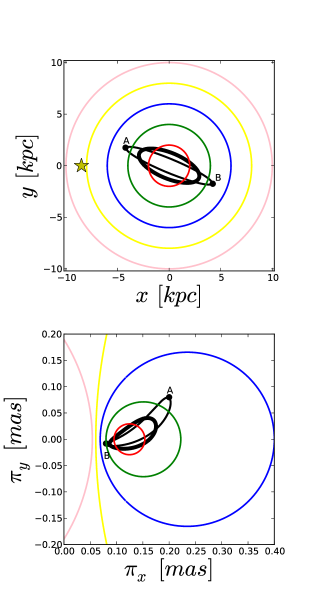
Figure 12: Mapping structures to the Gaia observable space. Top panel: structures in the $(x,y)$ configuration space. We plot in thick (thin) black lines the ellipses corresponding to the Boxy/bulge (Long) bar and galactocentric circles at 2(red), 4(green), 6(blue), 8(yellow) and 10(pink) kpc. The star symbol show the position of the Sun. Bottom panel: the same structures mapped in the ($(\pi_{x},\pi_{y})$) plane.

In Figure 13 we map the stellar surface density of the RC-all sample in the $(\pi_{x},\pi_{y})$ plane. We choose a square grid from $0.-0.26$mas in order to include all the bar structure as seen in Fig. 12 and of $2.6$ $\mu$as of width, which is of the order of Gaia’s resolution. As in Fig. 3, we discard stars with $R>10$kpc. Due to the relation between distance and parallax, the overdensity in the parallax plane does not directly correspond to the overdensity in the configuration space. In Fig. 13, we can observe how the particles organize in the expected structures of the bottom panel of Fig. 12. The far side of the bar and the far side of the Galaxy concentrates at smaller parallaxes, while the near side of the bar is more diffuse at higher parallaxes. Nevertheless, we still observe the tilted deformation corresponding to the near side of the bar at $\pi_{x}\in(0.15,0.2)$mas.

The following procedure enables us to subtract the axisymmetric component in the $(\pi_{x},\pi_{y})$ plane: 1) We “axisymmetrize” the original distribution of test particles in the configuration space. To obtain this “axisymmetrized” distribution, we convert the $(x,y)$ coordinates of each particle to $(R,\theta)$. We keep the $R$, but we substitute $\theta$ by a random number between $0$ and $2\pi$. And we convert back to $(x,y)$ coordinates. 2) We transform the “axisymmetrized” distribution to the parallax plane and we count the particles in each cell ($N_{a}$). 3) We subtract from the original distribution of test particles in the parallax plane ($N_{o}$) the one from the “axisymmetrized” distribution ($N_{a}$). When using this strategy to the RC-all sample, we can see in Fig. 13 (bottom panel) that the non-axisymmetric component, i.e. the Galactic bar, is well enhanced in the $(\pi_{x},\pi_{y})$.

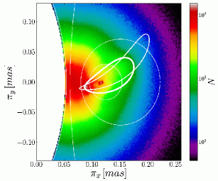
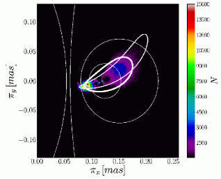
Figure 13: Mapping the RC-all sample in the parallax observable space. Top: We plot the whole sample. Note that the colour bar is in log scale. Bottom: We plot only the non-axisymmetric component. Note that the colour bar is linear counts, N, per area of size $2.6\mu as^{2}$. In both plots we over-plot the structure given by the Bulge ellipsoid (thick white line), the Long ellipsoid (thin white line) and circles of radius $2$, $4$, $8$ and $10\,kpc$, respectively from inside out, to help the reader guide in the figure. Note the different colour scale in the plots.

Figure 14 top shows the parallax plane for the RC-G20 sample, i.e. using real parallaxes with no errors (left panels), and the RC-G20-O sample, i.e. parallaxes affected by Gaia errors (right panels). The middle panels show the “axisymmetrized” distribution and the bottom panels show the result of subtracting the “axisymmetrized” distribution (middle panel) from the original one (top panel), that is, the bottom panels show the non-axisymmetric components in the parallax plane. A dominant feature is worth mentioning here, that is, the spikes in surface density at constant galactic longitude $l$ correspond to galactic longitudes with high visual absorption in the Drimmel extinction map (Drimmel, Cabrera-Lavers & López-Corredoira, 2003). Secondly, and more important, the effect of introducing the Gaia errors is clearly seen when we compare both columns. When we introduce the Gaia astrometric error in parallax each star expands symmetrically in the direction of constant longitude. This is not the case in configuration space, because of the fact that the error distribution in parallax translates into a skewed error distribution in distance (see Fig. 5). This effect is clearly observed in Fig. 14 right panels. First, and as an example, the overdensity seen in the top left panel, close to the $l=0^{\circ}$ galactic longitude (gray ellipse) is spread all over the $\pi_{x}$ axis when the Gaia errors are introduced. Second, it introduces an artificial effect when we want to subtract the axisymmetric component because the stars affected by error in parallax are not symmetrically shuffled in galactocentric radius, which translates in a distorted “axisymetrized” distribution (see middle right panel of Fig. 14). Therefore, the visual detection of the Galactic bar when Gaia parallax errors are considered is not possible. The relative error in parallax in the near side of the bar is too big – up to 40-70%– that the signature of the bar is lost. Once stated the difficulty to recover the Galactic bar characteristics in the RC-G20-O sample, even after subtracting the axisymmetric component, we consider that more complex methods are required, such as image reconstruction techniques. As a first step in this direction, in the next Sect. 4.2 we take the RC-G20-IR sample, with IR additional information, so more accurate distances.

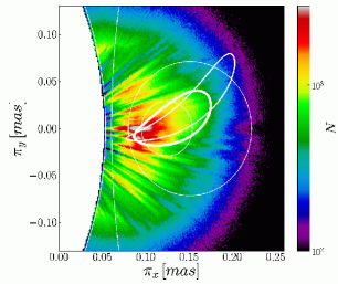
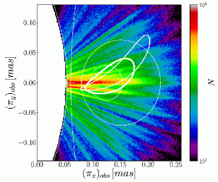
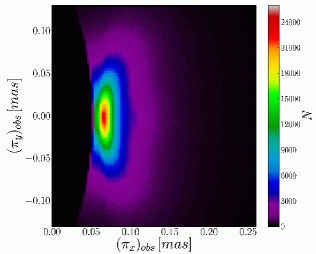
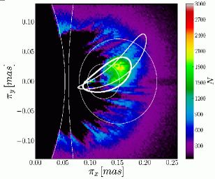
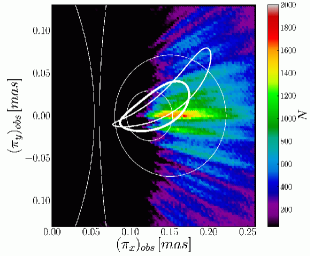
Figure 14: Mapping the RC-G20 sample in the parallax observable space. Top panels: RC-G20 sample, i.e. parallaxes without errors (left) and RC-G20-O sample, i.e. parallaxes with Gaia errors (right). Middle panels: The “axisymmetrized” distribution for the RC-G20 (left) and the RC-G20-O (right) samples. Bottom panels: the non-axisymmetric components of the samples, as the results of subtracting the “axisymmetrized” distributions (second row) from the original distributions (top row). Note that the colour bar is in log scale (in the top panels) and in linear scale (in the middle and bottom panels) and they are counts, N, per area of size $2.6\mu as^{2}$. Note, also, that they do not have the same scale. We overplot in the top and bottom panels the structure given by the Boxy/bulge ellipsoid (thick white line), the Long ellipsoid (thin white line) and circles of radius $2$, $4$, $8$ and $10$kpc, respectively from inside out, to help the reader guide in the figure. We show only data within $R<10$kpc in all panels.

Finally we have to take into account that the method applied above to model the axixymmetric compoment could cause non-negligible over- and under-substraction when applied to the RC-G20 and RC-G20-O samples. Due to the observational constraints, namely the cut in apparent magnitude (so distance) and the important dust extinction in the galactic plane, these samples present an important irregular surface density around a given galactocentric ring. Large foreground extinction along a given line-of-sight direction would reduce the total number of observed stars, thus, the substraction of a mean axisymmetric component will be overestimated in this position. On the contrary, areas well sampled by Gaia will have an under-substraction of the axisymmetric component as other parts of the ring are not well sampled, so the mean axisymmetric component is lower than the real one. Despite this drawback, this does not prevent from detecting the Galactic bar when using IR photometric distances.

4.2 The angular orientation of the Galactic bar using IR data

Working in the configuration space and using IR distances, we are interested in not only detecting the Galactic bar but also determining its angular orientation. In Fig. 15 we show the spheric volume density, $\rho_{S}$, as a function of the heliocentric distance for the RC-all (top panel) and the RC-G20-IR (bottom panel) samples for several lines-of-sight. We select the stars within $l\pm 2^{\circ}$ and in distance bins of $500$pc, we then divide the number of stars by the difference of volume of the spherical wedges of two consecutive distance bins. This is, $\rho=N_{s}/V$, where $N_{s}$ is the number of stars,

$$V=\frac{\alpha}{360}\frac{4\pi}{3}\left(d_{i+1}^{3}-d_{i}^{3}\right),$$ (1)

$\alpha=4^{\circ}$ is the solid angle of the wedge and $d_{i}$ and $d_{i+1}$ are distances of two consecutive bins in parsecs. Using the RC-all sample, we see that at $l=15^{\circ}$, we can clearly see the bar overdensity at about $6$kpc from the Solar position, while at $l=25^{\circ}$, there is no overdensity. This is also determined using the RC-G20-IR sample with IR errors. Note that the bar overdensity is detected from $l=15^{\circ}$ towards inner lines-of-sight. Even though these plots are useful to detect the bar overdensity, they are not precise or robust enough to determine the angular orientation of the bar.

Figure 15: Volume density as a function of the heliocentric distance at different lines-of-sight (with a solid angle of $4^{\circ}$). Top panel: lines-of-sight ($l=15$ in red and $l=25$ in green) for the RC-all sample. Bottom panel: five lines-of-sight ($l=5$ in cyan, $l=10$ in blue, $l=15$ in red, $l=20$ in black and $l=25$ in green) for the RC-G20-IR sample.

We then develop a method to determine the azimuthal angle of the bar overdensity in our Gaia samples following two steps. First, we subtract the axisymmetric component to enhance the bar structure, and, second, we perform a Gaussian fit to the subtracted stellar overdensity to locate the angular position of the maximum stellar density. The procedure is as follows:

1. Subtraction of the axisymmetric component. We make galactocentric radial bins of $100$pc and we compute the mean surface density inside each ring. We then subtract the mean from the initial surface density map. From that we obtain an image with the non-axisymmetric components clearly enhanced (see top panel of Fig. 16 for the RC-all sample).

2. Gaussian fit to the surface stellar overdenity. We make galactocentric polar bins of $400$pc in radius and $0.72^{\circ}$ of azimuthal width. For each radial ring, we fit a Gaussian function to the data using least squares. This allows us to derive the galactocentric azimuth at which the function has an absolute maximum (the mean of the fitted Gaussian). The error bar assigned to the azimuth of the maximum density is the $1\sigma$ error derived from the least square of the Gaussian fit.

This procedure has been applied to the RC-all and RC-G20-IR samples (Figs. 16 and 17). The RC-all sample allows us to check the performance of the method. In the top panel of Fig. 16, we show the surface density resulting after the subtraction of the axisymmetric part and the black dots are the result of the Gaussian fit. We perform the Gaussian fit to the stars in the first heliocentric quadrant ($0\leq l\leq 90^{\circ}$), which is where the near side of the Galactic bar is located. As expected, we clearly detect the Galactic bar, but we also highlight the inner ring and the response spiral arms due to the presence of the invariant manifolds (Romero-Gómez et al. , 2007). Note that the black dots follow the bar semi-major axis up to $R\sim 4$kpc, which corresponds to a radius intermediate between the one of the boxy/bulge bar and the one of the Long bar. This is more clearly shown in polar coordinates in Fig. 17. The azimuthal angle is defined positively in the counter-clockwise direction from the x-positive axis. Thus, the points line up along the $160^{\circ}$ constant azimuthal angle. The discrepancy at the end of the bar is clearly observed after $R>3.5$kpc associated to the overdensity of the inner ring and the spiral arms. This discrepancy would indicate approximately the length of the bar.

We then apply the same procedure to the RC-G20-IR sample (see bottom panel of Fig. 16). First, note that again, the extinction blurs the contribution of the non-axisymmetric components to the surface density. However, we still can observe the near side of the Galactic bar. If we examine this in polar coordinates (red curve in Fig. 17), we note the good recovery of the bar azimuthal angle. We observe a small bias of $\sim 3-5^{\circ}$, deviated with respect to the nominal value in about $2-3\sigma$. Several factors account for this bias. First, the RC-G20-IR sample has the effects of the extinction model. Given a certain line-of-sight, the number of stars observed will decrease with the heliocentric distance. This fact can translate into a change of the bar maximum observed density towards higher values of $\theta$. Second, the fact that the RC-G20-IR sample is magnitude-limited makes that intrinsically brighter stars are over-represented, this is the Malmquist bias. This can also lead to biased values of the azimuthal angle, which are not trivial to correct (Arenou & Luri, 2002). Third, there is also a geometric bias due to the fact that even having a symmetric error in photometric distance along the line of sight, it translates into a non-symmetric $\Delta\theta$ from the Galactic Centre. Only stars in a line-of-sight perpendicular to the semi-major axis of the bar will not suffer from this bias. In any case, even taking into account the possible biases, the Gaussian fit method recovers well the azimuthal angle of the Galactic bar.

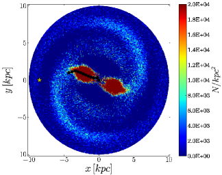
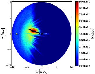
Figure 16: Determination of the bar azimuthal angle. Top panel: RC-all sample with the axisymmetric component subtracted. Bottom panel: RC-G20-IR sample also with the axisymmetric component subtracted. The back dots show the result of the Gaussian fit in the determination of the bar azimuth. Note that the scale of the colour bar is different in both panels.

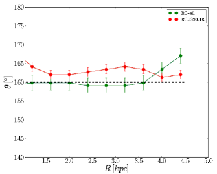
Figure 17: Determination of the bar azimuthal angle. We show in polar coordinates the result of the Gaussian fit to the RC-all sample (green curve) and RC-G20-IR sample (red curve). The horizontal thick black line corresponds to the imposed azimuthal angle in the model. The azimuth is defined positive counter-clockwise and from the x-positive axis. The bar, therefore, is located at $160^{\circ}$.

5 Conclusions

In this first paper of a series, we present two Red Clump Gaia mock catalogues. They are obtained as the integration of a set of test particles using a 3D barred galaxy model. We set the particles to mimic the characteristics of the disc RC giant stars and we use the Drimmel, Cabrera-Lavers & López-Corredoira (2003) extinction model with rescaling factors to obtain the apparent Gaia magnitudes $G$ and $G_{RVS}$ of the particles. Adding the Gaia error model available before commissioning for astrometry, photometry and spectroscopy, we obtain the corresponding observed catalogues, RC-G20-O and RC-RVS-O. The first catalogue, RC-G20-O, contains all particles observed by Gaia, i.e. we only apply a cut in magnitude ($G<20$), which reduces the number of particles by a factor of 2 with respect to the particles initially generated. Thus, Gaia will observe about $2.6\times 10^{7}$ RC disc stars. The second catalogue, RC-RVS-O, includes a second cut by requiring that the errors in radial velocity are small, $\sigma_{V_{r}}\leq 10$km s^-1in the nominal performances. The number of particles of this sample is $8.5\times 10^{6}$. This second mock catalogue contains all the 6 coordinates of phase space with good precision, since at an heliocentric distance of $4$kpc, the mean errors in tangential and radial velocity are, respectively, $\sim 20$km s^-1close to the Galactic plane and $\sim 10$km s^-1above $|z|>300$pc and $\sim 6$km s^-1close to the Galactic plane and $\sim 4$km s^-1, again above $|z|>300$pc.

We present a first attempt to describe the Galactic bar in the Gaia observable space, this is the cartesian projection of the $(\pi,l)$ coordinates $(\pi_{x},\pi_{y})=(\pi\cos l,\pi\sin l)$. We first analyse how the Galactic bar is projected in this space and then we apply this transformation to the RC-G20-O sample. We conclude that the Gaia relative errors in parallax and the high interstellar extinction in the inner parts of the Galactic disc prevent us to model the bar overdensity. This space is the natural space to directly see the effect of the extinction and we confirm the difficulties of Gaia, which works in the optical, to trace the bar structure without a robust statistical treatment.

This result points towards the need to combine Gaia and IR data to undertake the study of the internal disc structures. Since RC stars photometric distance has a better precision using IR surveys, we convolve the Gaia RC-G20 catalogue with a constant relative error in distance (we assume $10\%$ as in APOGEE (Bovy et al. , 2014)), obtaining the RC-G20-IR sample. In this case, the quality of the distances is good enough to clearly detect the bar overdensity, as seen in Figs. 16 and 17, and to allow an estimation of the bar angular orientation with an accuracy of $\sim 5^{\circ}$. In this work we quantify how the combination of surveys opens new avenues for the studies of the Galactic disc, in particular of the signatures of the Galactic bar.

The tool presented here can be adapted to any type of star. The study of the Galactic bar considering only the RC stars population has proven to be complex. However, Gaia will detect intrinsically brighter and redder late type giant stars, such as $M$ giant stars, with better accuracy than the RC stars at the same position. Assuming $M_{V}=-0.4$ and $(V-I_{c}=1.78)$ as in (2014), it gives for a star at about $4$kpc from the Sun, a $\sigma_{\pi}\sim 20\mu$as, and a relative error in parallax of about $5\%$, using the before commissioning error model. This good precision could help improving and complementing this work in detecting the Galactic bar overdensity.

The signature of the bar is present not only in density but it also shows imprints on the kinematic space, i.e. forming moving groups (e.g. Dehnen, 2000; Fux, 2001; Gardner & Flynn, 2010; Minchev et al. , 2010; Antoja et al. , 2011). Therefore, with Gaia, we are not limited to the study of the bar overdensity, but we can use all the 6D phase space. We are currently working on the analysis of the moments of the velocity distribution function in the Gaia sphere, about $4-5$kpc from the Sun, to try to obtain information on the potential of the Galaxy (Romero-Gómez et al, in preparation).

In this work, we have made the first attempts in evaluating the future Gaia data of RC stars and the capabilities of simple tools to recover the characteristics of the Galactic bar overdensity. Future work has to be done in developing appropriate tools, such as the application of statistically robust image reconstruction techniques in the space of the Gaia observables, where the contribution of the error can be easily accounted for.

Appendix A The generation of the Initial Conditions

The initial conditions follow the density distribution of the Miyamoto & Nagai (1975) disc, because this is the density distribution chosen in Allen & Santillán (1991) to characterise the disc of the Galaxy. The fact that the parameters of the disc defining the initial conditions are the same as the disc of the axisymmetric component used in the integration facilitates the relaxation of the particles. Particles generated using a mass distribution similar to the mass distribution imposed in the integration reach statistical equilibrium faster. The initial conditions are generated using the Hernquist method (, 1993). Here we summarize the steps:

A.1 Radial distribution

We first compute the normalized cumulative distribution function

$$\S^{*}(R)=\frac{1}{\Sigma_{0}}\int_{0}^{R}\Sigma^{*}(R^{\prime})dR^{\prime},$$ (2)

where $\Sigma^{*}(R)=R\int_{-\infty}^{+\infty}\rho(R,z)dz$ is the probability distribution function in cylindrical coordinates for the radial component, $\Sigma_{0}$ is the normalization constant, taken as $\Sigma_{0}=\int_{0}^{+\infty}\Sigma^{*}(R^{\prime})dR^{\prime}$, and $\rho(R,z)$ is the density of the Miyamoto-Nagai disc.

Once we have the normalized cumulative distribution function for a discrete set of radii, we use its inverse to generate the radial positions. Once we have the galactocentric distance of the star, R, we can obtain the cartesian coordinates $(x,y)$ by generating a random number in $[0,2\pi)$ and applying the polar coordinate transformation.

A.2 Vertical distribution

The generation of the vertical coordinate $z$ is performed in a similar way as in § A.1. The distribution function in z is derived from the integration of the vertical Jeans equation, for the particular case when $\sigma_{z}^{2}=\sigma_{z}^{2}(R)$, i.e. the vertical velocity dispersion only depends on $R$. For a given radius, $R$, the probability distribution function for the coordinate $z$ is

$$\nu(R,z)=e^{\Delta\Phi(z)/\sigma_{z}^{2}(R)},$$ (3)

where $\Delta\Phi(z)=\Phi(R,0)-\Phi(R,z)$ and $\Phi(R,z)$ is the Miyamoto- Nagai potential, and $\sigma_{z}^{2}(R)$ is the vertical velocity dispersion taken as, $\sigma_{z}^{2}(R)=\pi Gz_{0}\Sigma(R)$, where $z_{0}$ is the scale-length in z, considered constant here (as a first approximation of the solution) and $\Sigma(R)$ is the Miyamoto-Nagai surface density, computed numerically.

To randomly obtain the coordinate $z$, we use the Von Neumann Rejection Technique using this probability distribution function (Press et al. , 1992).

A.3 Generating the velocities

Now we need to generate the velocities associated to the positions generated above. First we define the radial, tangential and vertical dispersions.

As for the radial velocity dispersion, it consists of setting the square of the velocity dispersion proportional to the surface density and normalizing to a given value. We fix the value of $\sigma_{U}$ at a the Solar radius. This gives:

$$\sigma_{U}(R)=\sigma_{U}(R_{\odot})\left(\frac{\Sigma(R)}{\Sigma(R_{\odot})}\right)^{1/2}.$$ (4)

Note that we are assuming that the radial scale-length is double that of the density distribution.

The tangential velocity dispersion, $\sigma_{V}$, is determined by assuming the epicyclic approximation, that is:

$$\frac{\sigma_{V}^{2}(R)}{\sigma_{U}^{2}(R)}=\frac{\kappa^{2}}{4\Omega^{2}},$$ (5)

where $\kappa$ is the epicyclic frequency, and $\Omega$ is the angular frequency, computed from the rotation curve of the Allen & Santillán (1991) potential.

Finally, the vertical velocity dispersion, $\sigma_{W}$, is also set to proportional to the square root of the surface density. This expression comes from the Jeans and Poisson equations, together with the Eddington approximation (no coupling between $R$ and $z$) and isothermality in the vertical direction, that is $\sigma_{W}$ is independent of $z$.

$$\sigma_{W}(R)=\left(\pi Gz_{0}\Sigma(R)\right)^{1/2},$$ (6)

where $z_{0}$ is the scale-height of the disc, here considered constant, and $\Sigma(R)$ is the surface density of the Miyamoto-Nagai disk.

We now generate residual velocity components of each particle at position $(R,z)$ with respect to the Regional Standard of Rest, $(U,V,W)$, using a Gaussian with the respective velocity dispersions. There is though one final step to consider. We need to add the circular velocity, according the Allen & Santillán (1991) potential, and subtract the asymmetric drift to the tangential component. The asymmetric drift is approximated as (Binney & Tremaine, 2008)

$$V_{a}=\frac{1}{2V_{c}}\left[\left(\frac{\kappa^{2}}{4\Omega^{2}}-1-\frac{R}{\Sigma}\frac{\partial\Sigma^{\prime}}{\partial R}\right)\sigma_{U}^{2}-R\frac{\partial\sigma_{U}^{2}}{\partial R}\right],$$ (7)

where $\Sigma^{\prime}$ is the Miyamoto-Nagai density cut at $z=0$ and $V_{c}$ is the circular velocity both at the given radius $R$.

References

- Abedi et al. (2014) Abedi, H., Mateu, C., Aguilar, L., Figueras, F., Romero-Gomez, M. 2014, MNRAS,
- Allen & Santillán (1991) Allen, C., Santillán, A. 1991, Revista Mexicana de Astronomia y Astrofisica, 22, 255
- Arenou & Luri (2002) Arenou, F., Luri, X. 2002, proceedings of the JD13: HIPPARCOS and the luminosity calibration of nearer stars, XXIVth General Assembly of the IAU, T. LLoyd Evans & J.-C. Mermilliod (eds.) ASP Conference Series, Vol. 12
- Alves (2000) Alves, D.R. 2000, ApJ, 539, 732
- Antoja et al. (2011) Antoja, T., Figueras, F., Romero-Gomez, M., Pichardo, B., Valenzuela, O., Moreno, E. 2011, MNRAS, 418, 1423
- Benjamin et al. (2005) Benjamin, R.A., Churchwell, E., Babler, B.L., Indebetouw, R., Meade, M.R., Whitney, B.A., Watson, C., Wolfire, M.G., Wolff, M.J., Ignace, R., Bania, T.M., Bracker, S., Clemens, D.P., Chomiuk, L., Cohen, M., Dickey, J.M., Jackson, J.M., Kobulnicky, H.A., Mercer, E.P., Mathis, J.S., Stolovy, S.R., Uzpen, B. 2005, ApJ, 630L, 149
- Binney & Tremaine (2008) Binney, J., Tremaine, S. 2008, Galactic Dynamics, Second Edition, Princeton Univ. Press, Princeton
- Bovy et al. (2014) Bovy, J., Nidever D.L., Rix, H.-W., et al. 2014, arXiv:1405.1032
- Brown, Arenou, van Leeuwen et al. (1997) Brown, A.G.A, Arenou, F., van Leeuwen, F., Lindegren. L., Luri, X. 1997, ESA SP-402, 63
- Cabrera-Lavers et al. (2007) Cabrera-Lavers, A., Hammersley, P.L., González-Fernández, C., López-Corredoira, M., Garzón, F., Mahoney, T. J. 2008, A& A, 465, 825
- Cardelli, Clayton & Mathis (1989) Cardelli, J.A., Clayton, G.C., Mathis, J.S. 1989, ApJ, 345, 245
- Czekaj et al. (2014) Czekaj, M., Robin, A.C., Figueras, F., Luri, X., Haywood, M. 2014, A& A,
- Dehnen & Binney (1998) Dehnen, W., Binney, J. 1998, MNRAS,298, 387
- Dehnen (2000) Dehnen, W., 2000, AJ, 119, 800
- Drimmel, Cabrera-Lavers & López-Corredoira (2003) Drimmel, R., Cabrera-Lavers, A., López-Corredoira, M., 2003, A& A, 409, 205
- Eisenstein et al. (2011) Eisenstein, D., Weinberg, D.H., Agol, E. et al. 2011, AJ, 142, 72
- Ferrers (1877) Ferrers N. M. 1877, Q.J. Pure Appl. Math., 14, 1
- Fux (2001) Fux, R., 2001, A& A, 373, 511
- Gardner & Flynn (2010) Gardner, E., Flynn, C. 2010, MNRAS, 405, 545
- Gerhard (2011) Gerhard, O. 2011, in Tumbling, twisting, and winding galaxies: Pattern speeds along the Hubble sequence, E. M. Corsini and V. P. Debattista (eds), Memorie della Societa‘Astronomica Italiana Supplement, v.18, p.185
- Gilmore et al. (2012) Gilmore, G., Randich, S., Asplund, M. et al. 2012, The Messenger, 147, 25
- Hammersley et al. (2000) Hammersley, P.L., Garzón, F., Mahoney, T.J., López-Corredoira, M., Torres, M.A.P. 2000, MNRAS, 317, L45
- (23) Hernquist, L., 1993, ApJS, 86, 389
- (24) Hunt,J.A.S., Kawata, D., 2014, MNRAS, 443, 2112
- (25) Jordi, C., Gebran, M., Carrasco, J. M., de Bruijne, J., Voss, H., Fabricius, C., Knude, J., Vallenari, A., Kohley, R., Mora, A., 2010, A&A, 523, A48
- Kunder et al. (2012) Kunder, A., Koch, A., Rich, R.M., de Propis, R. et al. 2012, AJ, 143, 57
- López-Corredoira et al. (2007) López-Corredoira, M., Cabrera-Lavers, A., Mahoney, T.J., Hammersley, P.L., Garzón, F., González-Fernández, C. 2007, AJ, 133, 154
- López-Corredoira et al. (2014) López-Corredoira, M., Abedi, H., Garzón, F., Figueras, F. 2014, A& A, in press (arXiv:1409.6222)
- Martinez-Valpuesta & Gerhard (2011) Martinez-Valpuesta, I.; Gerhard, O. 2011, ApJ, 734, L20
- Minchev et al. (2010) Minchev, I., Boily, C., Siebert, A., Bienaymé, O. 2010, MNRAS, 407, 2122
- Miyamoto & Nagai (1975) Miyamoto, M., Nagai, R. 1975, PASJ, 27, 533
- Monari et al. (2014) Monari, G., Helmi, A., Antoja, T., Steinmetz, M. 2014, MNRAS, 569, A69
- Paczynski & Stanek (1998) Paczynski, B., Stanek, K.Z. 1998, ApJL, 494, 219L
- Peacock (1983) Peacock, J.A. 1983, MNRAS, 202, 615
- Press et al. (1992) Press, W.H., Teukolsky, S.A., Vetterling, W.T., Flannery, B.P. 1992, Numerical Recipes, Second Edition, Volume 1, Cambridge Univ. Press, Cambridge
- Rich et al. (2007) Rich, R.M., Reitzel, D.B., Howard, C.D., Zhao, H., 2007, ApJ, 658L, 29R
- Robin & Creze (1986) Robin, A., Creze, M. 1986, A& A, 157, 71
- Roca-Fabrega et al. (2014) Roca-Fabrega, S., Antoja, T., Figueras, F., Valenzuela, O. Romero-Gomez, M. 2014, MNRAS, accepted
- Romero-Gómez et al. (2007) Romero-Gómez, M., Athanassoula, E., Masdemont, J.J., García-Gómez, C. 2007, A& A, 472, 63
- Romero-Gómez et al. (2011) Romero-Gómez, M., Athanassoula, E., Antoja, T., Figueras, F. 2012, MNRAS, 418, 1176
- Stanek & Garnavich (1998) Stanek, K. Z., Garnavich, P.M. 1998, ApJL, 503, 131L
- Steinmetz et al. (2006) Steinmetz, M., Zwitter, T., Siebert, A. et al. 2006, AJ, 132, 1645
- Udalski et al. (1998) Udalski, A., Pietrzyński, G., Woźniak, P. et al. 1998, ApJL, 509, 25L
- Williams et al. (2013) Williams, M.E.K., Steinmetz, M., Binney, J. et al. 2013, MNRAS, 436, 101
- Zasowski et al. (2013) Zasowski, G., Johnson, J.A., Frinchaboy, P.M. et al. 2013, AJ, 146, 81