Seesaw Models with Minimal Flavor Violation

Abstract

We explore realizations of minimal flavor violation (MFV) for leptons in the simplest seesaw models where the neutrino mass generation mechanism is driven by new fermion singlets (type I) or triplets (type III) and by a scalar triplet (type II). We also discuss similarities and differences of the MFV implementation among the three scenarios. To study the phenomenological implications, we consider a number of effective dimension-six operators that are purely leptonic or couple leptons to the standard-model gauge and Higgs bosons and evaluate constraints on the scale of MFV associated with these operators from the latest experimental information. Specifically, we employ the most recent measurements of neutrino mixing parameters as well as the currently available data on flavor-violating radiative and three-body decays of charged leptons,  $\mu\to e$  conversion in nuclei, the anomalous magnetic moments of charged leptons, and their electric dipole moments. The most stringent lower-limit on the MFV scale comes from the present experimental bound on  $\mu\to e\gamma$  and can reach 500 TeV or higher, depending on the details of the seesaw scheme. With our numerical results, we illustrate some important differences among the seesaw types. In particular, we show that in types I and III there are features which can bring about potentially remarkable effects which do not occur in type II. In addition, we comment on how one of the new effective operators can induce flavor-changing dilepton decays of the Higgs boson, which may be probed in upcoming searches at the LHC.

I Introduction

The standard model (SM) of particle physics has been immensely successful in describing a vast amount of experimental data at energies up to $\cal O$(100) GeV pdg . One of the major implications is that in the quark sector flavor-dependent new interactions beyond the SM can readily be ruled out if they give rise to substantial flavor-changing neutral currents (FCNC). This motivates the formulation of the principle of so-called minimal flavor violation (MFV), which postulates that the sources of all FCNC and $CP$ violation reside in SM renormalizable Yukawa couplings defined at tree level mfv1 ; D'Ambrosio:2002ex . The MFV framework offers a predictive and systematic way to explore new physics which does not conserve quark flavor and $CP$ symmetries.

The implementation of the MFV principle for quarks is straightforward, but for leptons there are ambiguities, as the SM by itself does not predict lepton-flavor violation. Since there is now compelling empirical evidence for neutrino masses and mixing pdg , it is of interest to formulate MFV in the lepton sector by incorporating ingredients beyond the SM that can account for this observation Cirigliano:2005ck . However, we lack knowledge regarding not only the origin of neutrino mass, but also the precise nature of massive neutrinos. They could be Dirac fermions, like the electron and quarks, as far as their spin properties are concerned. Alternatively, neutrinos being electrically neutral, there is also the possibility that they are Majorana particles. The mass-generation mechanisms and Yukawa couplings for the neutrinos in the two cases differ significantly. Since the MFV hypothesis is closely associated with Yukawa couplings, one expects that the resulting phenomenologies in the two scenarios are also different.

In the Majorana neutrino case, there have been studies in the literature on some aspects of MFV realizations in various seesaw scenarios Cirigliano:2005ck ; Cirigliano:2006su ; Branco:2006hz ; Davidson:2006bd ; Gavela:2009cd , especially in the well-known simplest models of types I, II, and  III  seesaw1 ; seesaw12 ; seesaw2 ; seesaw3 . In this work, we take another look at these three seesaw schemes to investigate the contributions of new interactions organized according to the MFV principle. We adopt a model-independent approach, where such contributions consist of an infinite number of terms which are built up from leptonic Yukawa couplings and their products. It turns out that the infinite series can be resummed into only 17 terms Colangelo:2008qp . This formulation allows one to have a much more compact understanding of the terms that pertain to a given process. We find that for the specific processes to be considered only a few of them are relevant. We apply this to extract lower limits on the scale of MFV in the three seesaw scenarios using the latest experimental data, including the existing bounds on flavor-violating leptonic processes and the most recent measurements of neutrino mixing parameters. Also, we will examine the similarities and differences among the three seesaw types in relation to their MFV phenomenologies. We demonstrate especially that in types I and III there are features which can bring about potentially remarkable effects which do not happen in type II.

The plan of this paper is as follows. In the next section, we describe the MFV framework for leptons in the case that neutrinos are Dirac fermions. In Section III, we discuss the implementation of the MFV principle in scenarios involving Majorana neutrinos with masses generated via the seesaw mechanism of types I, II, and III. This is applied in Section IV, where we explore some of the phenomenology with effective dipole operators involving leptons and the photon. We evaluate constraints on the MFV scale associated with these operators from currently available data on flavor-violating radiative decays of charged leptons,  $\mu\to e$  conversion in nuclei, flavor-violating three-body decays of charged leptons, and their anomalous magnetic moments and electric dipole moments. With our numerical results, we illustrate some striking differences among the three seesaw types. In Section V, we look at several other leptonic operators satisfying the MFV principle. One of them can cause flavor-violating decay of the Higgs boson, which is testable at the LHC. We make our conclusions in Section VI.

II Leptonic MFV with Dirac neutrinos

Let us begin by describing how to arrange interactions under the MFV framework for leptons assuming that neutrinos are of Dirac nature. Following the MFV hypothesis that renormalizable Yukawa couplings defined at tree level are the only sources of FCNC and $CP$ violation, we need to start with such couplings for the neutrinos and charged leptons. We slightly extend the SM by including three right-handed neutrinos which transform as $(1,1,0)$ under the SM gauge group  ${\cal G}_{\scriptscriptstyle\rm SM}={\rm SU}(3)_{C}\times$SU(2)${}_{L}\times$U(1)_Y.  The Lagrangian responsible for the lepton masses can then be written as

$${\cal L}_{\rm m}\,\,=\,\,-(Y_{\nu})_{kl}\,\overline{L}_{k,L\,}\nu_{l,R\,}\tilde{H}\,-\,(Y_{e})_{kl}\,\overline{L}_{k,L\,}E_{l,R\,}H\;+\;{\rm H.c.}\,,$$ (1)

where summation over  $k,l=1,2,3$  is implicit, $Y_{\nu,e}$ are Yukawa coupling matrices, $L_{k,L}$ represents left-handed lepton doublets, $\nu_{k,R}$ and $E_{k,R}$ denote right-handed neutrinos and charged leptons, $H$ is the Higgs boson doublet, and  $\tilde{H}=i\tau_{2}H^{*}$  involving the second Pauli matrix $\tau_{2}$. Under the SM gauge group, $L_{k,L}$, $E_{k,R}$, and $H$ transform as  $(1,2,-1/2)$,  $(1,1,-1)$,  and  $(1,2,1/2)$,  respectively.

The MFV hypothesis  D'Ambrosio:2002ex ; Cirigliano:2005ck implies that ${\cal L}_{\rm m}$ is formally invariant under the global group  U(3)${}_{L}\times$U(3)${}_{\nu}\times$U(3)${}_{E}=G_{\ell}\times$U(1)${}_{L}\times$U(1)${}_{\nu}\times$U(1)_E  with  $G_{\ell}=\rm SU$(3)${}_{L}\times$SU(3)${}_{\nu}\times$SU(3)_E.  This entails that $L_{k,L}$, $\nu_{k,R}$, and $E_{k,R}$ belong to the fundamental representations of the SU(3)_L,ν,E, respectively,

$$L_{L}\,\to\,V_{L}L_{L}\,,~{}~{}~{}~{}~{}~{}~{}\nu_{R}\,\to\,V_{\nu}\nu_{R}\,,~{}~{}~{}~{}~{}~{}~{}E_{R}\,\to\,V_{E}E_{R}\,,~{}~{}~{}~{}~{}~{}~{}V_{L,\nu,E}\,\in\,{\rm SU}(3)_{L,\nu,E}\,,$$ (2)

and under $G_{\ell}$ the Yukawa couplings transform in the spurion sense according to

$$Y_{\nu}\,\to\,V_{L}Y_{\nu}V^{\dagger}_{\nu}\,\,\sim\,\,(3,\bar{3},1)\,,~{}~{}~{}~{}~{}~{}~{}Y_{e}\,\to\,V_{L}Y_{e}V^{\dagger}_{E}\,\,\sim\,\,(3,1,\bar{3})\,.$$ (3)

Taking advantage of the requirement that the final effective Lagrangian be invariant under $G_{\ell}$, without loss of generality one can always work in the basis where $Y_{e}$ is diagonal,

$$Y_{e}\,\,=\,\,\frac{\sqrt{2}}{v}\,{\rm diag}\bigl{(}m_{e},m_{\mu},m_{\tau}\bigr{)}$$ (4)

with  $v\simeq 246$ GeV  being the Higgs’s vacuum expectation value (VEV), and $\nu_{k,L}$, $\nu_{k,R}$, $E_{k,L}$, and $E_{k,R}$ refer to the mass eigenstates. Consequently, one can express $L_{k,L}$ and $Y_{\nu}$ in terms of the Pontecorvo-Maki-Nakagawa-Sakata neutrino mixing matrix $U_{\scriptscriptstyle\rm PMNS}$ as

$$L_{k,L}\,=\left(\!\begin{array}[]{c}(U_{\scriptscriptstyle\rm PMNS})_{kl\,}\nu_{l,L}\vspace{2pt}\\ E_{k,L}\end{array}\!\right),~{}~{}~{}~{}~{}~{}~{}Y_{\nu}\,=\,\frac{\sqrt{2}}{v}\,U_{\scriptscriptstyle\rm PMNS}\,\hat{m}_{\nu}\,,~{}~{}~{}~{}\hat{m}_{\nu}\,=\,{\rm diag}\bigl{(}m_{1},m_{2},m_{3}\bigr{)}\,,$$ (7)

where $m_{1,2,3}$ are the light neutrino eigenmasses and in the standard parametrization pdg

$$U_{\scriptscriptstyle\rm PMNS}\,=\left(\!\begin{array}[]{ccc}c_{12\,}c_{13}&s_{12\,}c_{13}&s_{13}\,e^{-i\delta}\vspace{1pt}\\ -s_{12\,}c_{23}-c_{12\,}s_{23\,}s_{13}\,e^{i\delta}&~{}~{}c_{12\,}c_{23}-s_{12\,}s_{23\,}s_{13}\,e^{i\delta}{}{}&s_{23\,}c_{13}\vspace{1pt}\\ s_{12\,}s_{23}-c_{12\,}c_{23\,}s_{13}\,e^{i\delta}&-c_{12\,}s_{23}-s_{12\,}c_{23\,}s_{13}\,e^{i\delta}&c_{23\,}c_{13}\end{array}\right),$$ (11)

with $\delta$ being the Dirac $CP$-violation phase,  $c_{kl}=\cos\theta_{kl}$,  and  $s_{kl}=\sin\theta_{kl}$.

Based on the transformation properties of the fields and Yukawa spurions, one then uses an arbitrary number of Yukawa coupling matrices to put together $G_{\ell}$-invariant objects which can induce the desired FCNC and $CP$-violating interactions. Thus, for operators involving two lepton fields, the pertinent building blocks are

$$\overline{L}_{L}\gamma_{\alpha}\Delta_{l}L_{L}\;,~{}~{}~{}~{}\overline{\nu}_{R}\gamma_{\alpha}\Delta_{\nu 8}\nu_{R}\;,~{}~{}~{}~{}\overline{E}_{R}\gamma_{\alpha}\Delta_{e8}E_{R}\;,~{}~{}~{}~{}\overline{\nu}_{R}\bigl{(}1,\sigma_{\alpha\beta}\bigr{)}\Delta_{\nu}L_{L}\;,~{}~{}~{}~{}\overline{E}_{R}\bigl{(}1,\sigma_{\alpha\beta}\bigr{)}\Delta_{e}L_{L}\;.$$ (12)

For these to be $G_{\ell}$ invariant, the $\Delta$’s should transform according to

$$\Delta_{l} \sim (1\oplus 8,1,1)\;,~{}~{}~{}~{}\Delta_{\nu 8}\,\sim\,(1,1\oplus 8,1)\;,~{}~{}~{}~{}\Delta_{e8}\,\sim\,(1,1,1\oplus 8)\;,$$

$$\Delta_{\nu} \sim (\bar{3},3,1)\;,\hskip 34.44434pt\Delta_{e}\,\sim\,(\bar{3},1,3)\;.$$ (13)

Since  $\overline{L}_{L}\gamma_{\alpha}\Delta_{l}L_{L}$,  $\overline{\nu}_{R}\gamma_{\alpha}\Delta_{\nu 8}\nu_{R}$,  and  $\overline{E}_{R}\gamma_{\alpha}\Delta_{e8}E_{R}$  must be Hermitian, $\Delta_{l,\nu 8,e8}$ must be Hermitian as well. To be acceptable terms in the Lagrangian, the above objects should be combined with appropriate numbers of other SM fields into singlets under the SM gauge group, with all the Lorentz indices contracted.

The MFV principle dictates that these $\Delta$’s are built up from the Yukawa coupling matrices $Y_{\nu,e}$ and $Y_{\nu,e}^{\dagger}$. Let us first discuss a nontrivial $\Delta$ which transforms as $(1\oplus 8,1,1)$ under $G_{\ell}$ and consists of terms in powers of

$${\sf A}\,\,=\,\,Y_{\nu}Y^{\dagger}_{\nu}\,\,=\,\,\frac{2}{v^{2}}\,U_{\scriptscriptstyle\rm PMNS\,}\hat{m}_{\nu}^{2}U_{\scriptscriptstyle\rm PMNS}^{\dagger}\;,~{}~{}~{}~{}~{}~{}~{}{\sf B}\,\,=\,\,Y_{e}Y_{e}^{\dagger}\,\,=\,\,\frac{2}{v^{2}}\,{\rm diag}\bigl{(}m_{e}^{2},m_{\mu}^{2},m_{\tau}^{2}\bigr{)}\,,$$ (14)

both of which also transform as $(1\oplus 8,1,1)$. Formally, $\Delta$ is a sum of infinitely many terms,  $\Delta=\sum\xi_{jkl\cdots\,}{\sf A}^{j}{\sf B}^{k}{\sf A}^{l}\cdots$  with coefficients $\xi_{jkl\cdots}$ expected to be at most of ${\cal O}$(1). Under the MFV framework, these coefficients must be real because otherwise they would introduce new sources of $CP$ violation beyond those in the Yukawa couplings. With the Cayley-Hamilton identity  $X^{3}=X^{2}\,{\rm Tr}X+\mbox{$\frac{1}{2}$}_{\,}X\bigl{[}{\rm Tr}X^{2}-({\rm Tr}X)^{2}\bigr{]}+\openone{\rm Det}X$  for an invertible 3$\times$3 matrix $X$, one can resum the infinite series into a limited number of terms Colangelo:2008qp ,

$$\Delta \,=\, \xi_{1}\openone+\xi_{2\,}{\sf A}+\xi_{3\,}{\sf B}+\xi_{4\,}{\sf A}^{2}+\xi_{5\,}{\sf B}^{2}+\xi_{6\,}{\sf AB}+\xi_{7\,}{\sf BA}+\xi_{8\,}{\sf ABA}+\xi_{9\,}{\sf BA}^{2}+\xi_{10\,}{\sf BAB}$$ (15)

$$\!+~{}\xi_{11\,}{\sf AB}^{2}+\xi_{12\,}{\sf ABA}^{2}+\xi_{13\,}{\sf A}^{2}{\sf B}^{2}+\xi_{14\,}{\sf B}^{2}{\sf A}^{2}+\xi_{15\,}{\sf B}^{2}{\sf AB}+\xi_{16\,}{\sf AB}^{2}{\sf A}^{2}+\xi_{17\,}{\sf B}^{2}{\sf A}^{2}{\sf B}~{},~{}~{}~{}$$

where $\openone$ stands for the 3$\times$3 unit matrix. Though one starts with all $\xi_{jkl\cdots\,}$ being real, the resummation process generally renders the coefficients $\xi_{r}$ in Eq. (15) complex due to imaginary parts created among the traces of the matrix products  ${\sf A}^{j}{\sf B}^{k}{\sf A}^{l}\cdots$  with  $j+k+l+\cdots\geq 6$  after the application of the Cayley-Hamilton identity. The imaginary contributions turn out to be reducible to factors proportional to a Jarlskog invariant quantity,  ${\rm Im\,Tr}\bigl{(}{\sf A}^{2}{\sf BAB}^{2}\bigr{)}=(i/2)\,{\rm Det}[{\sf A,B}]$,  which is much smaller than unity Colangelo:2008qp .

With Eq. (15), one can devise the objects in Eq. (II). Thus, the first of the Hermitian combinations can be  $\Delta_{l}=\Delta+\Delta^{\dagger}$.  To obtain nontrivial $\Delta_{\nu,e}$, one can take  $\Delta_{\nu}=Y_{\nu}^{\dagger}\Delta$  and  $\Delta_{e}=Y_{e}^{\dagger}\Delta$.  The construction of $\Delta_{\nu 8,e8}$ can be carried out in a similar way, except $\sf A$ and $\sf B$ are replaced by  $\tilde{A}=Y_{\nu}^{\dagger}Y_{\nu}$  and  $\tilde{B}=Y_{e}^{\dagger}Y_{e}$.  Since $\tilde{A}$ and $\tilde{B}$ are diagonal, so are any powers of them. Therefore, $\Delta_{\nu 8,e8}$ do not produce any FCNC and $CP$-violation effects.

We end this section by mentioning that the above discussion can be easily applied to the quark sector with the renormalizable Yukawa Lagrangian given by

$${\cal L}_{\rm m} \,=\, -(Y_{u})_{kl}\,\overline{Q}_{k,L\,}U_{l,R\,}\tilde{H}-(Y_{d})_{kl}\,\overline{Q}_{k,L\,}D_{l,R\,}H\;+\;{\rm H.c.}\,,$$ (16)

where $Y_{u,d}$ are Yukawa coupling matrices, $Q_{k,L}$ represents left-handed quark doublets, and $U_{k,R}$ $(D_{k,R})$ denote right-handed up-type (down-type) quarks. These fields transform as  $(3,2,1/6)$,  $(3,1,2/3)$,  and  $(3,1,-1/3)$,  respectively, under the SM gauge group ${\cal G}_{\scriptscriptstyle\rm SM}$. In the basis where $Y_{d}$ is diagonalized,

$$Y_{d}\,\,=\,\,\frac{\sqrt{2}}{v}\,{\rm diag}\bigl{(}m_{d},m_{s},m_{b}\bigr{)}\,,~{}~{}~{}~{}~{}~{}~{}Y_{u}\,\,=\,\,\frac{\sqrt{2}}{v}\,V^{\dagger}_{\scriptscriptstyle\rm{CKM}}\,\hat{m}_{u}\,,~{}~{}~{}~{}\hat{m}_{u}\,\,=\,\,{\rm diag}\bigl{(}m_{u},m_{c},m_{t}\bigr{)}\,,$$ (17)

where $V_{\scriptscriptstyle\rm CKM}$ is the Cabibbo-Kobayashi-Maskawa matrix which has the same standard parametrization as in Eq. (11). For MFV interactions, employing $Y_{u,d}$ along with  ${\sf A}=Y_{u}Y^{\dagger}_{u}$  and  ${\sf B}=Y_{d}Y^{\dagger}_{d}$  as building blocks, one can construct objects such as $\Delta_{q}$, $\Delta_{u}$, and $\Delta_{d}$, which are the quark counterparts of $\Delta_{l}$, $\Delta_{\nu}$, and $\Delta_{e}$, respectively He:2014fva .

III Seesaw models with MFV

If neutrinos are Majorana particles, the Yukawa couplings that take part in generating their masses differ from those in the Dirac neutrino case and depend on the model details. In this section we discuss how to realize the MFV hypothesis in the well-motivated seesaw models. The seesaw mechanism endows neutrinos with Majorana mass and provides a natural explanation for why they are much lighter than their charged partners. If just one kind of new particle is added to the minimal SM, there are three different scenarios seesaw1 ; seesaw12 ; seesaw2 ; seesaw3 : the famous seesaw models of type I, type II, and type III. A crucial step in the implementation of MFV in a given model is to identify the quantities $\sf A$ and $\sf B$ in terms of the relevant Yukawa couplings. This will be the emphasis of the section.

III.1 MFV in type-I seesaw model

In the type-I seesaw model, the SM is slightly expanded with the inclusion of three gauge-singlet right-handed neutrinos, $\nu_{k,R}$, which each carry a lepton number of 1 and are allowed to possess Majorana masses seesaw1 . The renormalizable Lagrangian for the lepton masses is

$${\cal L}_{\rm m}^{\rm I}\,\,=\,\,-(Y_{\nu})_{kl}\,\overline{L}_{k,L\,}\nu_{l,R\,}\tilde{H}-(Y_{e})_{kl}\,\overline{L}_{k,L\,}E_{l,R\,}H-\mbox{$\frac{1}{2}$}\,(M_{\nu})_{kl}\,\overline{\nu^{\rm c}_{k,R}}\,\nu_{l,R}\;+\;{\rm H.c.}\,,$$ (18)

where  $M_{\nu}={\rm diag}(M_{1},M_{2},M_{3})$  contains the right-handed neutrinos’ Majorana masses, breaking lepton-number symmetry, and  $\nu^{\rm c}_{k,R}\equiv(\nu_{k,R})^{\rm c}$,  the superscript c referring to charge conjugation. Accordingly, the masses of the neutral fermions make up the 6$\times$6 matrix

$${\sf M}\,\,=\,\,\left(\begin{array}[]{cc}0&M_{\rm D}\vspace{2pt}\\ M_{\rm D}^{\rm T}&M_{\nu}\end{array}\right)$$ (21)

in the $\bigl{(}U_{\scriptscriptstyle\rm PMNS}^{*}(\nu_{L})^{\rm c},\nu_{R}\bigr{)}{}^{\rm T}$ basis, where  $M_{\rm D}=vY_{\nu}/\sqrt{2}$.  If the nonzero elements of $M_{\nu}$ are much greater than those of $M_{\rm D}$, the seesaw mechanism becomes operational seesaw1 , resulting in the light neutrinos’ mass matrix

$$m_{\nu}\,\,=\,\,-\frac{v^{2}}{2}\,Y_{\nu}M_{\nu}^{-1}Y_{\nu}^{\rm T}\,\,=\,\,U_{\scriptscriptstyle\rm PMNS\,}\hat{m}_{\nu\,}U_{\scriptscriptstyle\rm PMNS}^{\rm T}\;,$$ (22)

where now $U_{\scriptscriptstyle\rm PMNS}$ contains the diagonal matrix  $P={\rm diag}(e^{i\alpha_{1}/2},e^{i\alpha_{2}/2},1)$  multiplied from the right, with $\alpha_{1,2}$ being the $CP$-violating Majorana phases. It follows that $Y_{\nu}$ in Eq. (7) is no longer valid, and one can instead pick $Y_{\nu}$ to be Casas:2001sr

$$Y_{\nu}\,\,=\,\,\frac{i\sqrt{2}}{v}\,U_{\scriptscriptstyle\rm PMNS\,}\hat{m}^{1/2}_{\nu}OM_{\nu}^{1/2}\,,$$ (23)

where $O$ is a matrix satisfying  $OO^{\rm T}=\openone$.  Since $O$ can be complex, it is a potentially important new source of $CP$ violation besides $U_{\scriptscriptstyle\rm PMNS}$.

Another implication of the presence of $M_{\nu}$ is that it will introduce an additional source of flavor violation if the masses $M_{1,2,3}$ of the right-handed neutrinos, $\nu_{k,R}$, are unequal  Davidson:2006bd . In that case, the extra flavor spurions should generally be taken into account by adding their contributions to $\Delta$ in  Eq. (15). However, if $\nu_{k,R}$ have the same mass,  $M_{1,2,3}={\cal M}$,  no new terms will need to be included in Eq. (15). In our treatment of the type-I seesaw with MFV, we restrict ourselves to this least complicated possibility that the right-handed neutrinos are degenerate. It follows that in this instance the flavor symmetry is  Cirigliano:2005ck  $G_{\ell}=\rm SU$(3)${}_{L}\times$O(3)${}_{\nu}\times$SU(3)_E,  under which  $\nu_{R}\to{\cal O}_{\nu}\nu_{R}$  and  $Y_{\nu}\to V_{L}Y_{\nu}{\cal O}_{\nu}^{\rm T}$,  where ${\cal O}_{\nu}$ is an orthogonal real matrix.

Moreover, from Eq. (23) with  $M_{\nu}={\cal M}\openone$  and $O$ being real or complex  Cirigliano:2005ck ; Branco:2006hz

$${\sf A}\,\,=\,\,Y_{\nu}Y^{\dagger}_{\nu}\,\,=\,\,\frac{2\cal M}{v^{2}}\,U_{\scriptscriptstyle\rm PMNS\,}\hat{m}^{1/2}_{\nu}OO^{\dagger}\hat{m}^{1/2}_{\nu}U_{\scriptscriptstyle\rm PMNS}^{\dagger}\;,$$ (24)

whereas  ${\sf B}=Y_{e}Y_{e}^{\dagger}$  in Eq. (14) is unchanged. These matrices are to be incorporated into the MFV objects mentioned earlier, such as $\Delta_{l,\nu,e}$. We note that, since  $\tilde{A}=Y^{\dagger}_{\nu}Y_{\nu}=(2{\cal M}/v^{2})O^{\dagger}\hat{m}_{\nu}O$,  here $\Delta_{\nu 8}$ is no longer diagonal, but it pertains only to $\nu_{R}$ interactions.

Now, in the Dirac neutrino case, $\sf A$ is given by Eq. (14) and therefore has tiny elements. In contrast, if $\cal M$ is sufficiently large, the eigenvalues of $\sf A$ in Eq. (24) can be sizable. Nevertheless, since as an infinite series $\Delta$ has to converge, $\cal M$ cannot be arbitrarily large Colangelo:2008qp ; He:2014fva . Accordingly, in numerical work we require the biggest eigenvalue of $\sf A$ to be unity, which implies that the elements of $\sf B$  are comparatively much smaller.

III.2 MFV in type-II seesaw model

The type-II seesaw model extends the SM with the addition of only one scalar SU(2)_L triplet given by seesaw12 ; seesaw2

$$T\,\,=\,\,\left(\begin{array}[]{cc}T^{+}/\sqrt{2}&T^{++}\vspace{1pt}\\ T^{0}&-T^{+}/\sqrt{2}\end{array}\right)$$ (27)

which transforms as $(1,3,1)$ under the SM gauge group ${\cal G}_{\scriptscriptstyle\rm SM}$. Accordingly, the Lagrangian describing the Yukawa couplings of leptons is

$${\cal L}_{\rm m}^{\rm II}\,\,=\,\,-(Y_{e})_{kl}\,\overline{L}_{k,L\,}E_{l,R\,}H\,-\,\mbox{$\frac{1}{2}$}\,(Y_{T})_{kl}\,\overline{L}_{k,L\,}\tilde{T}\,\big{(}L_{l,L}\big{)}^{\rm c}\;+\;{\rm H.c.}\,,$$ (28)

with  $\tilde{T}=i\tau_{2}T^{*}$.  It respects lepton-number conservation if $T$ is assigned a lepton number of $-2$. After the VEV of the neutral component of $T$ becomes nonzero,  $\bigl{\langle}T^{0}\bigr{\rangle}=v_{T}/\sqrt{2}$,  one obtains in ${\cal L}_{\rm m}^{\rm II}$ the neutrino mass matrix

$$m_{\nu}\,\,=\,\,\mbox{$\frac{1}{\sqrt{2}}$}\,v_{T\,}Y_{T}\,\,=\,\,U_{\scriptscriptstyle\rm PMNS\,}\hat{m}_{\nu\,}U_{\scriptscriptstyle\rm PMNS}^{\rm T}$$ (29)

in the basis where the charged lepton’s Yukawa coupling matrix, $Y_{e}$, has been diagonalized. If the nonzero elements of $Y_{T}$ are of $\cal O$(1), the tiny size of neutrino masses then comes from the suppression of $v_{T}$ due to certain choices of the parameters in the scalar potential $\cal V$. One can express it as Gelmini:1980re

$${\cal V} \,=\, -M_{H\,}^{2}H^{\dagger}H+M_{T\,}^{2}{\rm Tr}(T^{\dagger}T)+\mbox{$\frac{1}{2}$}\lambda_{1\,}(H^{\dagger}H)^{2}+\mbox{$\frac{1}{2}$}\lambda_{2\,}[{\rm Tr}(T^{\dagger}T)]^{2}+\lambda_{3\,}H^{\dagger}H\,{\rm Tr}(T^{\dagger}T)$$ (30)

$$\!+\;\lambda_{4\,}{\rm Det}(T^{\dagger}T)+\lambda_{5\,}H^{\dagger}T^{\dagger}TH\,-\,\mbox{$\frac{1}{\sqrt{2}}$}\bigl{(}\mu_{T}\,\tilde{H}^{\dagger}T^{\dagger}H\,+\,\mu_{T}^{*}\,H^{\dagger}T\tilde{H}\bigr{)}\,,$$

where  $M_{H}^{2}>0$  and  $M_{T}^{2}>0$.  The $\mu_{T}$ part explicitly breaks lepton-number symmetry and causes $T^{0}$ to develop a nonzero VEV. From the minimization of $\cal V$, one gets

$$\lambda_{1}v^{2}\,\,=\,\,2M_{H}^{2}+2|\mu_{T}|v_{T}-\lambda_{3}v_{T}^{2}\;,~{}~{}~{}~{}~{}~{}~{}|\mu_{T}|v^{2}\,\,=\,\,2M_{T\,}^{2}v_{T}+\lambda_{3}v^{2}v_{T}+\lambda_{2\,}v_{T}^{3}\;.$$ (31)

For  $|\mu_{T}|v_{T}\ll M_{H}^{2}$  and  $v_{T}\ll v$,  the first equality simplifies to  $\lambda_{1}v^{2}\simeq 2M_{H}^{2}$  like in the SM, and with the additional conditions  $v\ll M_{T}/|\lambda_{3}|^{1/2}$ and  $v_{T}\ll|\mu_{T}|$  the second relation in Eq. (31) translates into

$$v_{T}\,\,\simeq\,\,\frac{|\mu_{T}|v^{2}}{2M_{T}^{2}}\;,$$ (32)

which is small if  $|\mu_{T}|v\ll M_{T}^{2}$.  This turns into the seesaw form  $v_{T}\sim v^{2}/M_{T}$  if  $|\mu_{T}|\sim M_{T}\gg v$,  but the prerequisites just mentioned do not preclude a scenario with a relatively lighter triplet, in which $M_{T}$ can be as low as the TeV level Gavela:2009cd , provided that  $|\mu_{T}|\ll v$.

Since the triplet couples to SM gauge bosons, a nonzero $v_{T}$ will make the $\rho_{0}$ parameter deviate from unity Gelmini:1980re ,

$$\rho_{0}\,\,=\,\,\frac{m_{W}^{2}}{m_{Z\,}^{2}\cos^{2\!}\theta_{\rm W}}\,\,=\,\,\frac{v^{2}+2v_{T}^{2}}{v^{2}+4v_{T}^{2}}\,\,\simeq\,\,1\,-\,\frac{2v_{T}^{2}}{v^{2}}\;.$$ (33)

Its empirical value  $\rho_{0}=1.00040\pm 0.00024$ pdg then implies, at the 2$\sigma$ level, that  $v_{T}<1.6$ GeV.  This is much weaker than the requirement for the $v_{T}$ range that can produce neutrino masses of $\cal O$(0.1 eV) if the elements of $Y_{T}$ are of $\cal O$(1).

To implement the MFV hypothesis in this seesaw scheme, one observes that the Lagrangian in Eq. (28) possesses formal invariance under the global group  U(3)${}_{L}\times$U(3)${}_{E}=G_{\ell}^{\prime}\times$U(1)${}_{L}\times$U(1)_E,  with  $G_{\ell}^{\prime}=\rm SU$(3)${}_{L}\times$SU(3)_E,  if $L_{L}$ and $E_{R}$ belong to the fundamental representation of $SU(3)_{L,E}$, respectively,

$$L_{L}\,\to\,V_{L}L_{L}\,,~{}~{}~{}~{}~{}~{}~{}E_{R}\,\to\,V_{E}E_{R}\,,~{}~{}~{}~{}~{}~{}~{}V_{L,E}\,\in\,{\rm SU}(3)_{L,E}\,,$$ (34)

and the Yukawa couplings are spurions transforming according to

$$Y_{e}\,\to\,V_{L}Y_{e}V^{\dagger}_{E}\,,~{}~{}~{}~{}~{}~{}~{}Y_{T}\,\to\,V_{L}Y_{T}V_{L}^{\rm T}\,.$$ (35)

Here the building block $\Delta$ still has the expression in Eq. (15), with  ${\sf B}=Y_{e}Y_{e}^{\dagger}$  being the same as in Eq. (14), but unlike before

$${\sf A}\,\,=\,\,Y_{T}Y_{T}^{\dagger}\,\,=\,\,\frac{2}{v_{T}^{2}}\,U_{\scriptscriptstyle\rm PMNS\,}\hat{m}_{\nu\,}^{2}U_{\scriptscriptstyle\rm PMNS}^{\dagger}\,,$$ (36)

where from Eq. (29)

$$Y_{T}\,\,=\,\,\frac{\sqrt{2}}{v_{T}}\,U_{\scriptscriptstyle\rm PMNS\,}\hat{m}_{\nu\,}U_{\scriptscriptstyle\rm PMNS}^{\rm T}\,.$$ (37)

It is interesting to notice that $\sf A$ in Eq. (36) is the same as its Dirac-neutrino counterpart in Eq. (14), up to an overall factor. Due to this difference, whereas the elements of the latter are tiny, those in Eq. (36) can be of ${\cal O}(1)$ if $v_{T}$ is similar in order of magnitude to the neutrino masses. This will in fact be realized in our numerical analysis, as we will again choose the largest eigenvalue of $\sf A$ to be unity, which amounts to imposing  $v_{T}=\sqrt{2}\;{\rm max}\bigl{(}m_{1},m_{2},m_{3}\bigr{)}$.

Compared to Eq. (24) in the type-I case, $\sf A$ in Eq. (36) is in general much simpler. In particular, it no longer depends on the Majorana phases in $U_{\scriptscriptstyle\rm PMNS}$ which have canceled out due to $\hat{m}_{\nu}$ being diagonal and does not involve the $O$ matrix which can supply potentially major extra effects including $CP$-violating ones He:2014fva .

III.3 MFV in type-III seesaw model

In the type-III seesaw model, the new particles consist only of three fermionic SU(2)_L triplets seesaw3

$$\Sigma_{k}\,\,=\,\left(\!\begin{array}[]{cc}\Sigma_{k}^{0}/\sqrt{2}&\Sigma_{k}^{+}\vspace{2pt}\\ \Sigma_{k}^{-}&-\Sigma_{k}^{0}/\sqrt{2}\end{array}\!\right),~{}~{}~{}~{}~{}~{}~{}k\,\,=\,\,1,2,3\,,$$ (40)

which transform as $(1,3,0)$ under the SM gauge group ${\cal G}_{\scriptscriptstyle\rm SM}$. The Lagrangian responsible for the lepton masses is then

$${\cal L}_{\rm m}^{\rm III}\,\,=\,\,-(Y_{e})_{kl}\,\overline{L}_{k,L\,}E_{l,R\,}H\,-\,\sqrt{2}\;(Y_{\Sigma})_{kl}\,\overline{L}_{k,L\,}\Sigma_{l\,}\tilde{H}\,-\,\mbox{$\frac{1}{2}$}\,(M_{\Sigma})_{kl}\,{\rm Tr}\bigl{(}\overline{\Sigma_{k}^{\rm c}}\,\Sigma_{l}\bigr{)}\;+\;{\rm H.c.}$$ (41)

where $\Sigma_{k}^{\rm c}$ is the charge conjugate of $\Sigma_{k}$. For convenience, we define the right-handed fields  ${\cal E}_{k,R}=\Sigma_{k}^{-}$  and  ${\cal N}_{k,R}=\Sigma_{k}^{0}$  and left-handed fields  ${\cal E}_{k,L}=\bigl{(}\Sigma_{k}^{+}\bigr{)}\raisebox{1.0pt}{${}^{\rm c}$}$  and  ${\cal N}_{k,L}=\bigl{(}\Sigma_{k}^{0}\bigr{)}\raisebox{1.0pt}{${}^{\rm c}$}$.  In terms of matrices containing them and SM leptons, one can express the mass terms in ${\cal L}_{\rm m}^{\rm III}$ after electroweak symmetry breaking as

$${\cal L}_{\rm m}^{\rm III}\,\,\supset\,\,-\bigl{(}\overline{E}_{L}~{}~{}~{}\overline{\cal E}_{L}\bigr{)}\left(\!\begin{array}[]{cc}M_{\ell}&\sqrt{2}\,M_{\rm D}\vspace{2pt}\\ 0&M_{\Sigma}\end{array}\!\right)\left(\!\begin{array}[]{c}E_{R}\vspace{2pt}\\ {\cal E}_{R}\end{array}\!\right)-\,\mbox{$\frac{1}{2}$}\,\bigl{(}\overline{\nu}_{L}^{\,\prime}~{}~{}~{}\overline{\cal N}_{L}\bigr{)}\left(\!\begin{array}[]{cc}0&M_{\rm D}\vspace{2pt}\\ M_{\rm D}^{\rm T}&M_{\Sigma}\end{array}\!\right)\left(\!\begin{array}[]{c}(\nu_{L}^{\prime})\mbox{${}^{\rm c}$}\vspace{2pt}\\ {\cal N}_{R}\end{array}\!\right)\,+\;{\rm H.c.}\,,~{}~{}$$ (50)

where  $M_{\ell}=vY_{e}/\sqrt{2}$  and  $M_{\rm D}=vY_{\Sigma}/\sqrt{2}$  are 3$\times$3 matrices and  $\nu_{L}^{\prime}=U_{\scriptscriptstyle\rm PMNS\,}\nu_{L}$.  For  $M_{\Sigma}\gg M_{\rm D}$  in their nonzero elements, a seesaw mechanism like that in type I becomes operational to generate the light neutrinos’ mass matrix

$$m_{\nu}\,\,=\,\,-\frac{v^{2}}{2}\,Y_{\Sigma}M_{\Sigma}^{-1}Y_{\Sigma}^{T}\,.$$ (51)

Hence it is tempting simply to write $Y_{\Sigma}$ in a similar way to $Y_{\nu}$ in type I,

$$Y_{\Sigma}\,\,=\,\,\frac{i\sqrt{2}}{v}\,U_{\scriptscriptstyle\rm PMNS\,}\hat{m}^{1/2}_{\nu}OM_{\Sigma}^{1/2}\,,$$ (52)

and use $Y_{e}$ in Eq. (4) like before.

One, however, needs to justify this approximation because the light charged leptons, $E_{k}$, mix with the heavy ones, ${\cal E}_{k}$, as can be deduced from Eq. (50). They are related to the mass eigenstates $E_{k}^{\prime}$ and ${\cal E}_{k}^{\prime}$ by

$$\left(\begin{array}[]{c}E_{\sf C}\vspace{2pt}\\ {\cal E}_{\sf C}\end{array}\right)=\left(\begin{array}[]{ccc}(U_{EE})_{\sf C}&&(U_{E\cal E})_{\sf C}\vspace{2pt}\\ (U_{{\cal E}E})_{\sf C}&&(U_{\cal EE})_{\sf C}\end{array}\right)\left(\begin{array}[]{c}E_{\sf C}^{\prime}\vspace{2pt}\\ {\cal E}_{\sf C}^{\prime}\end{array}\right),~{}~{}~{}~{}~{}~{}~{}{\sf C}\,\,=\,\,L,R\;.$$ (59)

This alters $U_{\scriptscriptstyle\rm PMNS}$ in Eq. (52) to  $(U_{EE})_{L}^{\dagger}U_{\scriptscriptstyle\rm PMNS}$  as well as $Y_{e}$ to  $(U_{EE})_{L}^{\dagger}Y_{e\,}(U_{EE})_{R}$.  At leading order Abada:2008ea ,  $(U_{EE})_{L}=\openone-M_{D}M^{-2}_{\Sigma}M_{D}^{\dagger}$  and  $(U_{EE})_{R}=\openone$  for  $M_{D}\ll M_{\Sigma}$.  Thus, the deviations of $(U_{EE})_{L,R}$ from the unit matrix are negligible, and the approximation of $Y_{\Sigma}$ in Eq. (52) is justified.

Since $M_{\Sigma}$ in Eq. (41) would introduce an additional source of flavor violation if the fermion triplets had unequal masses, in our treatment of type III with MFV, like in type  I, we restrict ourselves to the less complicated possibility that these fermions are degenerate,  $M_{\Sigma}={\cal M}\openone$.  Accordingly, here we only need to work with

$${\sf A}\,\,=\,\,Y_{\Sigma}Y^{\dagger}_{\Sigma}\,\,=\,\,\frac{2\cal M}{v^{2}}\,U_{\scriptscriptstyle\rm PMNS\,}\hat{m}^{1/2}_{\nu}OO^{\dagger}\hat{m}^{1/2}_{\nu}U_{\scriptscriptstyle\rm PMNS}^{\dagger}$$ (60)

and, as in the previous scenarios, $\sf B$ in Eq. (14), which are no different from those in type I, where $O$ may be real or complex  Cirigliano:2005ck ; Branco:2006hz . Also, we fix the biggest eigenvalue of $\sf A$ to one.

IV Leptonic dipole operators in seesaw models with MFV

Having set up the basics of the MFV realizations in the minimal seesaw models of types I, II, and III, we now study some of the phenomenological implications and point out possible differences among them. It is clear from the last section that as far as MFV phenomenology is concerned type I and type III will be virtually alike because, with the new fermion masses being far above the TeV level, the building blocks for the quantity $\Delta$ are the same in both cases. However, within the MFV context we expect that marked differences can materialize between these two models and type II.

To explore the phenomenological consequences of MFV, one can adopt an effective theory approach D'Ambrosio:2002ex ; Cirigliano:2005ck , assuming that the heavy degrees of freedom in the full theory have been integrated out. This is especially suitable for the seesaw scenarios under consideration, where the masses of the new particles are much greater than the energies of the processes which we examine in this paper. A number of higher-dimensional effective operators involving leptons have been listed in the leptonic MFV literature Cirigliano:2005ck ; Cirigliano:2006su . Here we focus on dimension-six operators which generate dipole interactions between the SM leptons and electroweak gauge bosons. We deal with several other leptonic operators in the next section.

The dipole operators of interest are Cirigliano:2005ck

$$O^{(e1)}_{RL}\,=\,g^{\prime}\overline{E}_{R}Y^{\dagger}_{e}\Delta_{\ell 1}\sigma_{\kappa\omega}H^{\dagger}L_{L}B^{\kappa\omega}~{}, O^{(e2)}_{RL}\,=\,g_{\,}\overline{E}_{R}Y^{\dagger}_{e}\Delta_{\ell 2\,}\sigma_{\kappa\omega}H^{\dagger}\tau_{a}L_{L}W_{a}^{\kappa\omega}~{},$$ (61)

where $W$ and $B$ stand for the usual SU(2)_L$\times$U(1)_Y gauge fields with coupling constants $g$ and $g^{\prime}$, respectively, $\tau_{a}$ are Pauli matrices, summation over  $a=1,2,3$  is implicit, and $\Delta_{\ell 1,\ell 2}$ have the same form as $\Delta$ in Eq. (15), but with generally different $\xi_{r}$. One can write the effective Lagrangian for $O^{(e1,e2)}_{RL}$ as

$${\cal L}_{\rm eff}\,\,=\,\,\frac{1}{\Lambda^{2}}\Bigl{[}O^{(e1)}_{RL}+O^{(e2)}_{RL}\Bigr{]}\;+\;{\rm H.c}.~{},$$ (62)

where $\Lambda$ is the scale of MFV and their own coefficients in this Lagrangian have been absorbed by the $\xi_{r}$ in their respective $\Delta$’s.

The terms in Eq. (62) with the photon have the general form

$${\cal L}_{E_{k}E_{l}\gamma}\,\,=\,\,\frac{\sqrt{\alpha\pi}}{\Lambda^{2}}\,\overline{E}_{k\,}\sigma_{\kappa\omega}\Bigl{\{}m_{E_{k}}(\Delta_{\ell})_{kl}+m_{E_{l}}(\Delta_{\ell})_{lk}^{*}-\Bigl{[}m_{E_{k}}(\Delta_{\ell})_{kl}-m_{E_{l}}(\Delta_{\ell})_{lk}^{*}\Bigr{]}\gamma_{5}\Bigr{\}}E_{l\,}F^{\kappa\omega}~{},$$ (63)

where  $\alpha\simeq 1/137$  is the fine-structure constant, $F^{\kappa\omega}$ denotes the electromagnetic field-strength tensor,  $(E_{1},E_{2},E_{3})=(e,\mu,\tau)$,  and hereafter  $\Delta_{\ell}=\Delta_{\ell 1}-\Delta_{\ell 2}$.  These interactions contribute to the flavor-changing decays  $E_{l}\to E_{k}\gamma,E_{k}E_{j}^{-}E_{j}^{+}$  and nuclear  $\mu\to e$  conversion, as well as to the anomalous magnetic moments ($g-2$) and electric dipole moments (EDMs) of charged leptons. We ignore the contributions from ${\cal L}_{\rm eff}$ to  $\mu\to e$  conversion and  $E_{l}\to E_{k}E_{j}^{-}E_{j}^{+}$  that are mediated by the $Z$ boson due to the suppression by its mass. The flavor-changing transitions and lepton EDMs have been searched for over the years, but with null results so far, leading to increasingly severe bounds on their rates. For the electron and muon $g-2$, the predictions and measurements have reached high precision which continues to improve, implying that the inferred room for new physics is small and progressively decreasing. Thus the experimental information on these processes can offer very stringent restrictions on the scale $\Lambda$ in Eq. (62). We address this in the rest of the section.

IV.1 Flavor-changing transitions and anomalous magnetic moments

We treat first observables that are not sensitive to $CP$-violating effects. In this case, we can retain no more than 3 of the 17 terms of $\Delta$ in Eq. (15), as the others are suppressed by comparison. Since we pick the largest eigenvalue of the $\sf A$ matrix to be one in order to enhance the impact of new physics, the elements of $\sf A$ are much greater than those of the $\sf B$ matrix, whose biggest eigenvalue is  $2m_{\tau}^{2}/v^{2}\simeq 1.0\times 10^{-4}$.  As a consequence, the matrix elements of the terms in Eq. (15) with at least one power of $\sf B$ are in general significantly smaller due to this suppression factor than the terms without any $\sf B$. Thus, in dealing with such observables, we can make the approximation  $\Delta=\xi_{1}\openone+\xi_{2\,}{\sf A}+\xi_{4\,}{\sf A}^{2}$,  leading to  $\Delta^{\dagger}=\Delta$  after the small ${\rm Im}_{\,}\xi_{1,2,4}$ have been ignored.

Among the flavor-changing decays  $E_{l}\to E_{k}\gamma$,  one can expect the most severe constraint from  $\mu\to e\gamma$  which has the strictest measured limit pdg . With its amplitude derived from Eq. (63), one determines its branching ratio to be

$${\cal B}(\mu\to e\gamma)\,\,=\,\,\frac{\alpha\tau_{\mu}m_{\mu}^{5}}{\Lambda^{4}}\bigl{|}(\Delta_{\ell})_{21}\bigr{|}\raisebox{1.0pt}{${}^{2}$}\,,$$ (64)

where $\tau_{\mu}$ is the muon lifetime, the electron mass has been neglected, and

$$(\Delta_{\ell})_{jk}\,\,=\,\,\xi_{2\,}^{\ell}{\sf A}_{jk}\,+\,\xi_{4\,}^{\ell}({\sf A}\raisebox{-0.7pt}{${}^{2}$})_{jk}\,.$$ (65)

From Eq. (64), one can easily obtain the corresponding formulas for  $\tau\to e\gamma$  and  $\tau\to\mu\gamma$  by appropriately changing the flavor indices. These tau decays can place complementary restraints on the dipole couplings.

Searches for  $\mu\to e$  conversion in nuclei can offer constraints on new physics competitive to those from  $\mu\to e\gamma$  measurements deGouvea:2013zba . Assuming that the flavor-changing transition is again due to the dipole operators alone, one can write the conversion rate in nucleus ${\cal N}$ as Kitano:2002mt

$${\cal B}(\mu{\cal N}\to e{\cal N})\,\,=\,\,\frac{\alpha\pi_{\,}m_{\mu\,}^{5}\bigl{|}(\Delta_{\ell})_{21}^{~{}~{}}D_{\cal N}\bigr{|}\raisebox{1.0pt}{${}^{2}$}}{\Lambda^{4\,}\omega_{\rm capt}^{\cal N}}\;,$$ (66)

where $D_{\cal N}$ is the dimensionless overlap integral for $\cal N$ and $\omega_{\rm capt}^{\cal N}$ the rate of $\mu$ capture in ${\cal N}$. Based on the existing experimental limits on  $\mu\to e$  transition in various nuclei pdg and the corresponding $D_{\cal N}$ and $\omega_{\rm capt}^{\cal N}$ values Kitano:2002mt , one expects that the data on  $\mu{\rm Ti}\to e{\rm Ti}$  and  $\mu{\rm Au}\to e{\rm Au}$  may supply important restrictions. To calculate their rates, we will employ  $D_{\rm Ti}=0.087$,  $D_{\rm Au}=0.189$,  $\omega_{\rm capt}^{\rm Ti}=2.59\times 10^{6}/\rm s$,  and  $\omega_{\rm capt}^{\rm Au}=13.07\times 10^{6}/\rm s$  Kitano:2002mt .

Another kind of flavor-changing process which receives contributions from the interactions in Eq. (63) is the three-body decay  $E_{l}\to E_{k}E_{j}^{-}E_{j}^{+}$.  If there are no other contributions, one can express its rate as

$$\Gamma_{E_{l}\to E_{k}E_{j}\bar{E}_{j}}\,\,=\,\,\frac{\alpha^{2}m_{E_{l}}^{5~{}}\bigl{|}(\Delta_{\ell})_{lk}\bigr{|}\raisebox{1.0pt}{${}^{2}$}}{4\pi_{\,}\Lambda^{4}}\;{\cal I}_{E_{l}\to E_{k}E_{j}\bar{E}_{j}}\,,$$ (67)

where the $m_{E_{k}}$ terms in Eq. (63) have been neglected and the factor ${\cal I}_{E_{l}\to E_{k}E_{j}\bar{E}_{j}}$, from the phase-space integration, can be calculated using formulas available in the literature Cirigliano:2006su . The factors relevant to the processes we will examine are  ${\cal I}_{\mu\to ee\bar{e}}=9.885$,  ${\cal I}_{\tau\to\mu\mu\bar{\mu}}=3.264$,  ${\cal I}_{\tau\to\mu e\bar{e}}=16.97$,   ${\cal I}_{\tau\to ee\bar{e}}=17.41$,  and ${\cal I}_{\tau\to e\mu\bar{\mu}}=3.01$.

For numerical analysis, we need in addition the values of the various neutrino parameters, especially their masses and the elements of the mixing matrix $U_{\scriptscriptstyle\rm PMNS}$. For these, we adopt the numbers quoted in Table  1 from a recent fit to global neutrino data Capozzi:2013csa . Most of them depend on whether neutrino masses fall into a normal hierarchy (NH) or an inverted one (IH). Since empirical information on the absolute scale of $m_{1,2,3}$ is still far from precise pdg , for definiteness we set  $m_{1}=0$ $(m_{3}=0)$  in the NH (IH) case. As for the Majorana phases $\alpha_{1,2}$, there are still no data available on their values.

Parameter	NH	IH
$\sin^{2}\theta_{12}$	$0.308\pm 0.017$	$0.308\pm 0.017\vphantom{\frac{1}{2}_{|}^{|}}$
$\sin^{2}\theta_{23}$	$0.437^{+0.033}_{-0.023}$	$0.455^{+0.139}_{-0.031}\vphantom{\frac{1}{2}_{|}^{|}}$
$\sin^{2}\theta_{13}$	$0.0234^{+0.0020}_{-0.0019}$	$0.0240^{+0.0019}_{-0.0022}\vphantom{\frac{1}{2}_{|}^{|}}$
$\delta/\pi$	$1.39^{+0.38}_{-0.27}$	$1.31^{+0.29}_{-0.33}\vphantom{\frac{1}{2}_{|}^{|}}$
$\delta m^{2}=m_{2}^{2}-m_{1}^{2}$	$\left(7.54^{+0.26}_{-0.22}\right)_{\vphantom{\int}}^{\vphantom{\int}}\times 10^{-5}\;\rm eV^{2}$	$\left(7.54_{-0.22}^{+0.26}\right)\times 10^{-5}\;\rm eV^{2}$
$\Delta m^{2}=\bigl{|}m_{3}^{2}-\bigl{(}m_{1}^{2}+m_{2}^{2}\bigr{)}/2\bigr{|}\vphantom{\int_{|_{|}}^{|^{|}}}$	$(2.43\pm 0.06)\times 10^{-3}\;\rm eV^{2}$	$(2.38\pm 0.06)\times 10^{-3}\;\rm eV^{2}$

Table 1: Results of a recent analysis of global three-neutrino oscillation data Capozzi:2013csa , in terms of best-fit values and allowed 1$\sigma$ ranges of the mass-mixing parameters. The neutrino mass hierarchy may be normal $\bigl{(}m_{1}<m_{2}<m_{3}\bigr{)}$ or inverted $\bigl{(}m_{3}<m_{1}<m_{2}\bigr{)}$.

To proceed, we also need to specify the $\sf A$ matrix, which is model dependent, as seen in the preceding section. For the type-I or -III seesaw scenario, $\sf A$ in Eq. (24) [or (60)] can have many different realizations, depending on $M_{\nu}$ and $O$. We consider first the least complicated possibility that the right-handed neutrinos $\nu_{k,R}$ are degenerate, with  $M_{\nu}={\cal M}\openone$,  and $O$ is a real orthogonal matrix, in which case

$${\sf A}\,\,=\,\,\frac{2\cal M}{v^{2}}\,U_{\scriptscriptstyle\rm PMNS\,}\hat{m}_{\nu\,}U_{\scriptscriptstyle\rm PMNS}^{\dagger}$$ (68)

with eigenvalues  $\hat{\sf A}_{1,2,3}=2{\cal M}m_{1,2,3}/v^{2}$.  Explicitly, including this in Eq. (65) yields

$$(\Delta_{\ell})_{21} \,=\, -c_{12\,}c_{13\,}\Bigl{(}s_{12\,}c_{23}+e^{i\delta\,}c_{12\,}s_{23\,}s_{13}\Bigr{)}\Bigl{(}\xi_{2\,}^{\ell}\hat{\sf A}_{1}+\xi_{4\,}^{\ell}\hat{\sf A}_{1}^{2}\Bigr{)}$$ (69)

$$\!+\;s_{12\,}c_{13\,}\Bigl{(}c_{12\,}c_{23}-e^{i\delta\,}s_{12\,}s_{23\,}s_{13}\Bigr{)}\Bigl{(}\xi_{2\,}^{\ell}\hat{\sf A}_{2}+\xi_{4\,}^{\ell}\hat{\sf A}_{2}^{2}\Bigr{)}$$

$$\!+\;e^{i\delta\,}s_{23\,}c_{13\,}s_{13}\,\Bigl{(}\xi_{2\,}^{\ell}\hat{\sf A}_{3}+\xi_{4\,}^{\ell}\hat{\sf A}_{3}^{2}\Bigr{)}_{\vphantom{\int}}\,,$$

$$(\Delta_{\ell})_{31} \,=\, c_{12\,}c_{13\,}\Bigl{(}s_{12\,}s_{23}-e^{i\delta\,}c_{12\,}c_{23\,}s_{13}\Bigr{)}\Bigl{(}\xi_{2\,}^{\ell}\hat{\sf A}_{1}+\xi_{4\,}^{\ell}\hat{\sf A}_{1}^{2}\Bigr{)}$$ (70)

$$\!-\;s_{12\,}c_{13\,}\Bigl{(}c_{12\,}s_{23}+e^{i\delta\,}s_{12\,}c_{23\,}s_{13}\Bigr{)}\Bigl{(}\xi_{2\,}^{\ell}\hat{\sf A}_{2}+\xi_{4\,}^{\ell}\hat{\sf A}_{2}^{2}\Bigr{)}$$

$$\!+\;e^{i\delta\,}c_{23\,}c_{13\,}s_{13}\,\Bigl{(}\xi_{2\,}^{\ell}\hat{\sf A}_{3}+\xi_{4\,}^{\ell}\hat{\sf A}_{3}^{2}\Bigr{)}_{\vphantom{\int}}\,,$$

$$(\Delta_{\ell})_{32} \,=\, -\Bigl{(}s_{12\,}c_{23}+e^{-i\delta\,}c_{12\,}s_{23\,}s_{13}\Bigr{)}\Bigl{(}s_{12\,}s_{23}-e^{i\delta\,}c_{12\,}c_{23\,}s_{13}\Bigr{)}\Bigl{(}\xi_{2\,}^{\ell}\hat{\sf A}_{1}+\xi_{4\,}^{\ell}\hat{\sf A}_{1}^{2}\Bigr{)}$$ (71)

$$\!-\;\Bigl{(}c_{12\,}c_{23}-e^{-i\delta\,}s_{12\,}s_{23\,}s_{13}\Bigr{)}\Bigl{(}c_{12\,}s_{23}+e^{i\delta\,}s_{12\,}c_{23\,}s_{13}\Bigr{)}\Bigl{(}\xi_{2\,}^{\ell}\hat{\sf A}_{2}+\xi_{4\,}^{\ell}\hat{\sf A}_{2}^{2}\Bigr{)}$$

$$\!+\;c_{23\,}s_{23\,}c_{13}^{2}\,\Bigl{(}\xi_{2\,}^{\ell}\hat{\sf A}_{3}+\xi_{4\,}^{\ell}\hat{\sf A}_{3}^{2}\Bigr{)}\,.$$

Later on we will also provide examples for a case in which $O$ is complex.

With $(\Delta_{\ell})_{kl}$ specified, we can determine lower limits on the MFV scale $\Lambda$ from the experimental information on the observables described above. The particular data we use are listed in the first two columns of Table 2. Since in our model-independent approach $\xi_{2,4}$ are free constants, for simplicity we assume that only one of them is nonzero at a time. For  $\xi_{4}=0$,  we scan the ranges of the neutrino mass and mixing parameters quoted in Table 1 in order to maximize $(\Delta_{\ell})_{21,32,31}$ separately, while ensuring that the values of $\cal M$ make  ${\rm max}\bigl{(}\hat{\sf A}_{1},\hat{\sf A}_{2},\hat{\sf A}_{3}\bigr{)}=1$.  This allows us extract the maximal lower-limits on  $\hat{\Lambda}=\Lambda/\bigl{|}\xi_{2}^{\ell}\bigr{|}{}^{1/2}$  from the measured bounds on ${\cal B}(\mu\to e\gamma)$, ${\cal B}(\tau\to\mu\gamma)$, and ${\cal B}(\tau\to e\gamma)$ listed in Table 2, which are the strictest ones to date in their respective groups of processes with the same flavor changes. Subsequently, we apply the acquired values of $(\Delta_{\ell})_{21,32,31}$ to obtain limits from the other experimental bounds in this table. We collect the $\hat{\Lambda}$ numbers in the third column which correspond to the NH (IH) of neutrino masses. For comparison, employing the central values in Table 1 would give us results which are smaller by up to 30%. It is worth mentioning that in all this computation the right-handed neutrino mass is  ${\cal M}\simeq\mbox{(6.0-6.3)}\times 10^{14}\;$GeV.

Observable	$\stackrel{{\scriptstyle\displaystyle\rm Experimental}}{{\rm upper~{}bound\vphantom{|^{|}}}}$	$\vphantom{|_{|}^{\int_{|}}}\hat{\Lambda}_{\rm min}/$TeV
		Types I and III	Type II
${\cal B}(\mu\to e\gamma)\vphantom{\frac{1}{2}_{|}^{|}}$	$5.7\times 10^{-13}$ pdg	338 (307)	294 (312)
${\cal B}(\mu{\rm Ti}\to e{\rm Ti})\vphantom{\frac{1}{2}_{|}^{|}}$	$6.1\times 10^{-13}$ Papoulias:2013gha	85 (77)	73 (78)
${\cal B}(\mu{\rm Au}\to e{\rm Au})\vphantom{\frac{1}{2}_{|}^{|}}$	$7.0\times 10^{-13}$ pdg	80 (73)	70 (74)
${\cal B}(\mu^{-}\to e^{-}e^{-}e^{+})\vphantom{\frac{1}{2}_{|}^{|}}$	$1.0\times 10^{-12}$ pdg	81 (74)	70 (75)
${\cal B}(\tau\to\mu\gamma)\vphantom{\frac{1}{2}_{|}^{|}}$	$4.4\times 10^{-8}$ pdg	22 (24)	23 (23)
${\cal B}(\tau^{-}\to\mu^{-}\mu^{-}\mu^{+})\vphantom{\frac{1}{2}_{|}^{|}}$	$2.1\times 10^{-8}$ pdg	5.6 (5.9)	5.9 (5.9)
${\cal B}(\tau^{-}\to\mu^{-}e^{-}e^{+})\vphantom{\frac{1}{2}_{|}^{|}}$	$1.8\times 10^{-8}$ pdg	8.7 (9.3)	9.2 (9.3)
${\cal B}(\tau\to e\gamma)\vphantom{\frac{1}{2}_{|}^{|}}$	$3.3\times 10^{-8}$ pdg	15 (13)	13 (13)
${\cal B}(\tau^{-}\to e^{-}e^{-}e^{+})\vphantom{\frac{1}{2}_{|}^{|}}$	$2.7\times 10^{-8}$ pdg	4.9 (4.2)	4.3 (4.2)
${\cal B}(\tau^{-}\to e^{-}\mu^{-}\mu^{+})\vphantom{\frac{1}{2}_{|}^{|}}$	$2.7\times 10^{-8}$ pdg	3.2 (2.7)	2.8 (2.7)

Table 2: Lower limits on  $\hat{\Lambda}=\Lambda/\bigl{|}\xi_{2}^{\ell}\bigr{|}{}^{1/2}$  associated with dipole operators $O_{RL}^{(e1,e2)}$ inferred from experimental upper-bounds on the branching ratios of flavor-violating leptonic transitions, as explained in the text. In this and the remaining tables, the unbracketed (bracketed) results correspond to the normal (inverted) hierarchy of light neutrino masses with  $m_{1(3)}=0$.

For the type-II scheme, $\sf A$ is given only in Eq. (36), which has eigenvalues  $\hat{\cal A}_{1,2,3}=2m_{1,2,3}^{2}/v_{T}^{2}$  and leads to

$$(\Delta_{\ell})_{21} \,=\, -c_{12\,}c_{13\,}\Bigl{(}s_{12\,}c_{23}+e^{i\delta\,}c_{12\,}s_{23\,}s_{13}\Bigr{)}\Bigl{(}\xi_{2\,}^{\ell}\hat{\cal A}_{1}+\xi_{4\,}^{\ell}\hat{\cal A}_{1}^{2}\Bigr{)}$$ (72)

$$\!+\;s_{12\,}c_{13\,}\Bigl{(}c_{12\,}c_{23}-e^{i\delta\,}s_{12\,}s_{23\,}s_{13}\Bigr{)}\Bigl{(}\xi_{2\,}^{\ell}\hat{\cal A}_{2}+\xi_{4\,}^{\ell}\hat{\cal A}_{2}^{2}\Bigr{)}$$

$$\!+\;e^{i\delta\,}s_{23\,}c_{13\,}s_{13}\,\Bigl{(}\xi_{2\,}^{\ell}\hat{\cal A}_{3}+\xi_{4\,}^{\ell}\hat{\cal A}_{3}^{2}\Bigr{)}$$

and its $(\Delta_{\ell})_{31,32}$ counterparts, which are analogous to those in Eqs. (70) and (71), respectively. Utilising these matrix elements, we take steps similar to those elaborated in the previous paragraph, while adjusting $v_{T}$ such that  ${\rm max}\bigl{(}\hat{\cal A}_{1},\hat{\cal A}_{2},\hat{\cal A}_{3}\bigr{)}=1$,  in order to extract from data the lower limits on $\hat{\Lambda}$ for  $\xi_{4}^{\ell}=0$.  We collect the results in the fourth column of Table 2, which correspond to  $v_{T}\sim 0.07$ eV.  With  $\xi_{2}^{\ell}=0$  instead, we obtain comparable numbers for  $\Lambda_{\rm min}/|\xi_{4}^{\ell}|^{1/2}$,  specifically  285 (320) TeV  from the ${\cal B}(\mu\to e\gamma)$ data. Now, since  $2\hat{\cal A}_{k}{\cal M}^{2}v_{T}^{2}=\hat{\sf A}_{k}^{2}v^{4}$,  one realizes that the numbers in the fourth column of Table 2 are also the limits on  $\Lambda/|\xi_{4}^{\ell}|^{1/2}$  in the type-I case of the last paragraph with  $\xi_{2}^{\ell}=0$.

It is clear from Table 2 that to date the most stringent constraint on the dipole operators in Eq. (62) comes from the measured bound on  $\mu\to e\gamma$  among processes that change lepton flavor. It is instructive to entertain the consequence of this for the calculated branching ratios of the other transitions if other operators are absent or have only minor impact. Thus, employing the $\hat{\Lambda}_{\rm min}$ numbers belonging to ${\cal B}(\mu\to e\gamma)$ in Table 2 and the corresponding neutrino parameter values, we compute the results listed in Table 3. The ratios of any two of them and the relative size of any one of them with respect to ${\cal B}(\mu\to e\gamma)$ are, therefore, predictions of the particular scenario considered. They can be checked experimentally if two or more of these processes are detected in the future, as the presence of other operators with nonnegligible effects would likely lead to a different set of predictions. Since the numbers in Table 3 are at least two orders of magnitude below their current experimental bounds, it is of interest to make comparison with the projected sensitivities of future experiments on lepton flavor violation.

Observable	Prediction
	Types I and III	Type II
${\cal B}(\mu{\rm Ti}\to e{\rm Ti})\vphantom{\frac{1}{2}_{|}^{|}}$	$2.4\;(2.4)\times 10^{-15}$	$2.4\;(2.4)\times 10^{-15}$
${\cal B}(\mu{\rm Au}\to e{\rm Au})\vphantom{\frac{1}{2}_{|}^{|}}$	$2.2\;(2.2)\times 10^{-15}$	$2.2\;(2.2)\times 10^{-15}$
${\cal B}(\mu^{-}\to e^{-}e^{-}e^{+})\vphantom{\frac{1}{2}_{|}^{|}}$	$3.3\;(3.3)\times 10^{-15}$	$3.3\;(3.3)\times 10^{-15}$
${\cal B}(\tau\to\mu\gamma)\vphantom{\frac{1}{2}_{|}^{|}}$	$7.9\;(14)\times 10^{-13}$	$1.7\;(1.4)\times 10^{-12}$
${\cal B}(\tau^{-}\to\mu^{-}\mu^{-}\mu^{+})\vphantom{\frac{1}{2}_{|}^{|}}$	$1.5\;(2.7)\times 10^{-15}$	$3.3\;(2.6)\times 10^{-15}$
${\cal B}(\tau^{-}\to\mu^{-}e^{-}e^{+})\vphantom{\frac{1}{2}_{|}^{|}}$	$7.8\;(14)\times 10^{-15}$	$1.7\;(1.3)\times 10^{-14}$
${\cal B}(\tau\to e\gamma)\vphantom{\frac{1}{2}_{|}^{|}}$	$2.5\;(5.7)\times 10^{-14}$	$8.6\;(4.6)\times 10^{-14}$
${\cal B}(\tau^{-}\to e^{-}e^{-}e^{+})\vphantom{\frac{1}{2}_{|}^{|}}$	$2.5\;(5.7)\times 10^{-16}$	$8.7\;(4.7)\times 10^{-16}$
${\cal B}(\tau^{-}\to e^{-}\mu^{-}\mu^{+})\vphantom{\frac{1}{2}_{|}^{|}}$	$4.3\;(9.9)\times 10^{-17}$	$15\;(8.0)\times 10^{-17}$

Table 3: Predictions calculated from the contributions of the dipole operators alone, with the $\hat{\Lambda}_{\rm min}$ numbers from the experimental bound on ${\cal B}(\mu\to e\gamma)$ in Table 2 and the neutrino parameter values used to determine them.

There are planned searches for  $\mu\to e\gamma$  with projected sensitivity reaching a few times $10^{-14}$ within the next five years Cavoto:2014qoa . If they come up empty, the predictions in Table 3 will decrease somewhat, probably by up to an order of magnitude. Nevertheless, the prediction for  $\mu\to 3e$  in Table 3 will likely still be testable with new experiments looking for it which will start running in a couple of years and may be able to probe a branching ratio as low as $10^{-16}$ after several years CeiA:2014wea ; Mori:2014aqa . Complementary checks may be available from upcoming searches for flavor-violating tau decays which can improve their current empirical limits by two orders of magnitude CeiA:2014wea . Potentially severe restrictions will be supplied by future measurements on  $\mu\to e$  conversion in nuclei which will begin in a few years and are expected to achieve sensitivity at the level of $10^{-17}$ or better eventually CeiA:2014wea ; Mori:2014aqa .

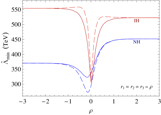
Figure 1: Variation of the lower limit on  $\hat{\Lambda}=\Lambda/|\xi_{2}^{\ell}|^{1/2}$,  subject to ${\cal B}(\mu\to e\gamma)$ data, versus complex-$O$ parameter  $\rho=r_{1}=r_{2}=r_{3}$  in the absence of the Majorana phases,  $\alpha_{1,2}=0$,  for  $\xi_{4}^{\ell}=0$  and degenerate $\nu_{k,R}$ (solid curves), as explained in the text. The dashed curves depict the corresponding variation of the lower limit on  $\Lambda/|\xi_{4}^{\ell}|^{1/2}$  for  $\xi_{2}^{\ell}=0$.

As another significant observation from Table 2, it indicates that no remarkable differences in the bounds on $\Lambda$ appear among the three types of seesaw models if in type I or III the right-handed neutrinos are degenerate and the $O$ matrix is real, with $\sf A$ in Eq. (68). If $O$ is complex and/or the right-handed neutrinos are nondegenerate, $\sf A$ is less simple which may give rise to more pronounced deviations from the type-II results. To illustrate this, we next explore the possibility that $O$ is complex.

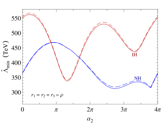
Figure 2: Variation of the lower limit on  $\hat{\Lambda}=\Lambda/|\xi_{2}^{\ell}|^{1/2}$,  subject to ${\cal B}(\mu\to e\gamma)$ data, versus $\alpha_{2}$ for  $\alpha_{1}=0$,  degenerate $\nu_{k,R}$, and complex-$O$ parameter  $\rho=r_{1}=r_{2}=r_{3}=-1$  (solid curves), as explained in the text. The dashed curves depict the corresponding variation of the lower limit on  $\Lambda/|\xi_{4}^{\ell}|^{1/2}$  for  $\xi_{2}^{\ell}=0$.

With $\nu_{k,R}$ still degenerate,  $M_{\nu}={\cal M}\openone$,  but $O$ complex, $\sf A$ is more complicated,

$${\sf A}\,\,=\,\,\frac{2}{v^{2}}\,{\cal M}_{\,}U_{\scriptscriptstyle\rm PMNS\,}\hat{m}^{1/2}_{\nu}OO^{\dagger}\hat{m}^{1/2}_{\nu}U_{\scriptscriptstyle\rm PMNS}^{\dagger}\;.$$ (73)

One can always write  $OO^{\dagger}=e^{2i\sf R}$  with a real antisymmetric matrix

$${\sf R}\,\,=\,\left(\begin{array}[]{ccc}0&r_{1}&r_{2}\vspace{1pt}\\ -r_{1}&0&r_{3}\vspace{1pt}\\ -r_{2}&~{}\mbox{$-r_{3}$}{}&0\end{array}\right).$$ (77)

Since $OO^{\dagger}$ is not diagonal, $\sf A$ generally has dependence on the Majorana phases in $U_{\scriptscriptstyle\rm PMNS}$ if they are not zero. To concentrate first on demonstrating how $O$ can bring about significant new effects, we switch off the Majorana phases,  $\alpha_{1,2}=0$.  Subsequently, for illustration, we pick  $r_{1}=r_{2}=r_{3}=\rho$  and again scan the parameter ranges in Table 1 in order to get the highest  $\Lambda/|\xi_{2,4}^{\ell}|^{1/2}$  from the experimental bound on ${\cal B}(\mu\to e\gamma)$, with the condition that the largest eigenvalue of $\sf A$ in Eq. (73) is unity. We exhibit the resulting dependence on $\rho$ in Figure 1. It reveals that, in this example, the contribution of $O$ can boost $\Lambda_{\rm min}$ by up to 80% with respect to its value when $O$ is real, which implies that the predicted branching ratio is enhanced by an order of magnitude.

Turning our attention now to the impact of the Majorana phases, we make the same choice of  $r_{1,2,3}=\rho$  as in the preceding paragraph, select  $\alpha_{1}=0$  and  $\rho=-1$,  and let $\hat{\Lambda}_{\rm min}$ vary as a function of $\alpha_{2}$, in similar steps to those in the last example. We display the variation in Figure 2, which shows that although the Majorana phases in this instance can increase the lower limits on $\Lambda$ only moderately, they can induce sizable reduction of it. Hence the associated decay rate is affected in roughly the same way. All these examples demonstrate that the $O$ matrix and Majorana phases in types I and III can produce striking effects which do not occur in type II.

Before finishing this subsection, we examine limitations from the anomalous magnetic moments, $a_{\ell}$, of charged leptons. The Lagrangian for $a_{\ell}$ is  ${\cal L}_{a_{\ell}}=\sqrt{\alpha\pi}\,a_{\ell}\,\overline{\ell}\sigma^{\kappa\omega}\ell F_{\kappa\omega}/\bigl{(}2m_{\ell}\bigr{)}$,  which gets contributions from the flavor-diagonal couplings in Eq. (63). Accordingly

$$a_{E_{k}}\,\,=\,\,\frac{4_{\,}m_{E_{k}}^{2}}{\Lambda^{2}}\,\bigl{[}\xi_{1\,}^{\ell}\delta_{kk}+\xi_{2\,}^{\ell}{\sf A}_{kk}+\xi_{4\,}^{\ell}({\sf A}\raisebox{-0.7pt}{${}^{2}$})_{kk}\bigr{]}\,,$$ (78)

where as earlier we have ignored the tiny ${\rm Im}_{\,}\xi_{1,2,4}^{\ell}$. Since $a_{e}$ is much suppressed by the electron mass, and since the measurement of $a_{\tau}$ is not yet precise pdg , the strongest restrictions from anomalous magnetic moments can be expected from $a_{\mu}$. Currently its experimental and SM values differ by  $a_{\mu}^{\rm exp}-a_{\mu}^{\scriptscriptstyle\rm SM}=(249\pm 87)\times 10^{-11}$ Aoyama:2012wk , which suggests that we can require the new contributions to satisfy  $\bigl{|}a_{\mu}\bigr{|}<3.4\times 10^{-9}$.  Assuming again that the right-handed neutrinos are degenerate and the $O$ matrix is real, if only one of $\xi_{1,2,4}^{\ell}$ is nonzero at a time, from this $a_{\mu}$ bound we infer  $\Lambda/|\xi_{1,2,4}^{\ell}|^{1/2}>3.6,2.7,2.5$ TeV.  Upon comparing these numbers with those in Table 2, we conclude that the muon $g\!-\!2$ cannot at present compete with the flavor-violating leptonic transitions in restraining $\Lambda$.

IV.2 Lepton EDMs

The interactions in Eq. (63) also contribute to a charged lepton’s electric dipole moment, denoted by $d_{\ell}$, which is a sensitive probe for the existence of new sources of $CP$ violation, as the SM prediction is very small He:1989xj . The Lagrangian for $d_{\ell}$ is  ${\cal L}_{d_{\ell}}=-(id_{\ell}/2)\overline{\ell}\sigma^{\kappa\omega}\gamma_{5}\ell F_{\kappa\omega}$,  and so

$$d_{E_{k}}\,\,=\,\,\frac{\sqrt{2}\,e_{\,}v}{\Lambda^{2}}\;{\rm Im}\bigl{(}Y^{\dagger}_{e}\Delta_{\ell}\bigr{)}_{kk}\;.$$ (79)

Unlike the observables treated in the previous subsection which are dominated by a few of the terms in $\Delta_{\ell}$ with lowest orders in the $\sf A$ and $\sf B$ matrices, the contributions pertinent to lepton EDMs are those from higher orders. Thus, for the electron we have He:2014fva

$$d_{e}\,\,=\,\,\frac{\sqrt{2}\,e_{\,}v}{\Lambda^{2}}\Bigl{[}\xi^{\ell}_{12}\,{\rm Im}\bigl{(}Y^{\dagger}_{e}{\sf ABA}{}^{2}\bigr{)}_{11}+\xi^{\ell}_{16}\,{\rm Im}\bigl{(}Y^{\dagger}_{e}{\sf AB}{}^{2}{\sf A}{}^{2}\bigr{)}_{11}\Bigr{]}\,,$$ (80)

where we have again neglected ${\rm Im}_{\,}\xi^{\ell}_{r}$. Hereafter we drop the $\xi^{\ell}_{16}$ part which is suppressed by one factor of $\sf B$ relative to the $\xi^{\ell}_{12}$ term. The very small number of them serves to illustrate the benefit of the resummation of the infinite series in $\Delta_{\ell}$ into the 17 terms, as in  Eq. (15).

The latest analysis on $d_{e}$ under the MFV framework has been performed in Ref. He:2014fva for the Dirac neutrino case as well as the type-I (and, hence, also type-III) seesaw model. If neutrinos are Dirac particles, $d_{e}$ has the form

$$d_{e}^{\rm D}\,\,=\,\,\frac{32e_{\,}m_{e}}{\Lambda^{2}v^{8}}\bigl{(}m_{\mu}^{2}-m_{\tau}^{2}\bigr{)}\bigl{(}m^{2}_{1}-m_{2}^{2}\bigr{)}\bigl{(}m_{2}^{2}-m_{3}^{2}\bigr{)}\bigl{(}m_{3}^{2}-m_{1}^{2}\bigr{)}\,\xi_{12\,}^{\ell}J_{\ell}\;,$$ (81)

where  $J_{\ell}={\rm Im}\bigl{(}U_{e2}U_{\mu 3}U_{e3}^{*}U^{*}_{\mu 2}\bigr{)}$  is a Jarlskog invariant for $U_{\scriptscriptstyle\rm PMNS}$. This turns out to be independent of the $m_{1,2,3}$ individually because the neutrino squared-mass differences defined in Table  1 imply that  $\bigl{(}m^{2}_{1}-m_{2}^{2}\bigr{)}\bigl{(}m_{2}^{2}-m_{3}^{2}\bigr{)}\bigl{(}m_{3}^{2}-m_{1}^{2}\bigr{)}=\delta m^{2}\bigl{(}\Delta m^{2}\bigr{)}\raisebox{1.0pt}{${}^{2}$}-\frac{1}{4}\bigl{(}\delta m^{2}\bigr{)}\raisebox{1.0pt}{${}^{3}$}$.  On the other hand, in types I and III with degenerate $\nu_{k,R}$ and a real $O$ matrix, in which case $\sf A$ is given by Eq. (68),

$$d_{e}^{\rm I,III}\,\,=\,\,\frac{32e_{\,}m_{e\,}{\cal M}^{3}}{\Lambda^{2}v^{8}}\bigl{(}m_{\mu}^{2}-m_{\tau}^{2}\bigr{)}\bigl{(}m_{1}-m_{2}\bigr{)}\bigl{(}m_{2}-m_{3}\bigr{)}\bigl{(}m_{3}-m_{1}\bigr{)}\,\xi_{12\,}^{\ell}J_{\ell}\;,$$ (82)

Since  $m_{k}\ll\cal M$,  one can see that $d_{e}^{\rm D}$ is considerably suppressed relative to $d_{e}^{\rm M}$. In contrast, for type II one derives

$$d_{e}^{\rm II}\,\,=\,\,\frac{32e_{\,}m_{e}}{\Lambda^{2}v^{2}v_{T}^{6}}\bigl{(}m_{\mu}^{2}-m_{\tau}^{2}\bigr{)}\bigl{(}m_{1}^{2}-m_{2}^{2}\bigr{)}\bigl{(}m_{2}^{2}-m_{3}^{2}\bigr{)}\bigl{(}m_{3}^{2}-m_{1}^{2}\bigr{)}\,\xi_{12\,}^{\ell}J_{\ell}\,\,=\,\,\biggl{(}\frac{v}{v_{T}}\biggr{)}^{\!\!6}d_{e}^{\rm D}\,,$$ (83)

which is far above $d_{e}^{\rm D}$ due to  $v_{T}\ll v$.  From these formulas, one can readily find those for $d_{\mu,\tau}$ by cyclically changing the mass subscripts.

Numerically,  $d_{e}^{\rm D}=1.3\times 10^{-99\;}e\,{\rm cm\,(GeV}/\hat{\Lambda})^{2}$  He:2014fva , which is too minuscule to yield any useful restraint on $\hat{\Lambda}$ from the newest data  $|d_{e}|_{\rm exp}<8.7\times 10^{-29\;}e$ cm  from the ACME experiment acme . In the Majorana neutrino case, the type-I (or -III) prediction in Eq. (82) has been evaluated in Ref. He:2014fva to yield the limit  $\hat{\Lambda}>0.36\,(0.12)\;{\rm TeV}$  corresponding to  ${\cal M}=6.16\,(6.22)\times 10^{14}$ GeV  for the NH (IH) of neutrino masses.

In type II, from Eq. (83) we arrive at

$$\frac{d_{e}^{\rm II}}{e\,\rm cm}\,\,=\,\,2.7\;(2.6)\times 10^{-31}\biggl{(}\frac{\rm eV}{v_{T}}\biggr{)}^{\!\!6}\biggl{(}\frac{\rm GeV}{\hat{\Lambda}}\biggr{)}^{\!\!2}$$ (84)

for the NH (IH) case. Then  $|d_{e}|_{\rm exp}<8.7\times 10^{-29\;}e$ cm  translates into

$$\hat{\Lambda}\,\,>\,\,0.055\;(0.054)\;{\rm GeV}\biggl{(}\frac{\rm eV}{v_{T}}\biggr{)}^{\!\!3}.$$ (85)

With  $v_{T}\simeq 0.069$ eV  from the requirement that the largest eigenvalue of ${\sf A}$ in Eq. (36) be unity, it follows that

$$\hat{\Lambda}\,\,>\,\,0.17\;\rm TeV\,,$$ (86)

which is roughly comparable to its counterparts in type I (or III) quoted above.

In the preceding discussion, $d_{e}$ is caused by the $CP$-violating Dirac phase $\delta$ in $U_{\scriptscriptstyle\rm PMNS}$, and the Majorana phases $\alpha_{1,2}$ therein do not take part. However, if $O$ is complex, the phases in it may give rise to an extra contribution to $d_{e}$ and the Majorana phases can modify it further. As investigated in detail in Ref. He:2014fva , these new $CP$-violating contributions to $d_{e}$ can be more important than those of $\delta$. Such effects do not occur in type II, as $d_{e}^{\rm II}$ does not have dependence on $O$ or $\alpha_{1,2}$.

V Additional leptonic operators

Besides the dipole operators, under the MFV framework there are other dimension-six operators, listed in Ref. Cirigliano:2006su , that can arise in the three simplest seesaw scenarios. Focusing on operators that are purely leptonic or couple leptons to the SM gauge and Higgs bosons, one can write

$${\cal L}_{\rm eff}^{\prime}\,\,=\,\,\frac{1}{\Lambda^{2}}\sum_{m=1}^{3}O_{4L}^{(m)}+\frac{1}{\Lambda^{2}}\Bigl{[}O_{RL}^{(e3)}\,+\,{\rm H.c.}\Bigr{]}+\frac{1}{\Lambda^{2}}\sum_{n=1}^{2}O_{LL}^{(n)}\,,$$ (87)

where

$$O^{(1)}_{4L} \,=\, \overline{L}_{L}\gamma^{\mu}\Delta_{\scriptscriptstyle 4L}^{\scriptscriptstyle(1)}L_{L}\,\overline{L}_{L}\gamma_{\mu}^{\;\;}\Delta_{\scriptscriptstyle 4L^{\prime}}^{\scriptscriptstyle(1)}L_{L}\,,\hskip 50.00008ptO^{(2)}_{4L}\,\,=\,\,\overline{L}_{L}\gamma^{\mu}\Delta_{\scriptscriptstyle 4L\,}^{(\scriptscriptstyle 2)}\tau_{a}L_{L}\,\overline{L}_{L}\gamma_{\mu}^{\;\;}\Delta_{\scriptscriptstyle 4L^{\prime}\,}^{\scriptscriptstyle(2)}\tau_{a}L_{L}\,,~{}~{}~{}~{}$$

$$O^{(3)}_{4L} \,=\, \overline{L}_{L}\gamma^{\mu}\Delta_{\scriptscriptstyle 4L}^{\scriptscriptstyle(3)}L_{L}\,\overline{E}_{R}^{~{}~{}}\gamma_{\mu}E_{R}\,,\hskip 60.00009pt\,O_{RL}^{(e3)}\,\,=\,\,({\cal D}_{\mu}H)^{\dagger\,}\overline{E}_{R}Y_{e}^{\dagger}\Delta_{\scriptscriptstyle RL\,}{\cal D}^{\mu}L_{L}\,,$$

$$O^{(1)}_{LL} \,=\, \mbox{$\frac{i}{2}$}\bigl{[}H^{\dagger}({\cal D}_{\mu}H)-({\cal D}_{\mu}H)^{\dagger}H\bigr{]}\overline{L}_{L}\gamma^{\mu}\Delta_{\scriptscriptstyle LL}^{\scriptscriptstyle(1)}L_{L}\,,$$

$$O^{(2)}_{LL} \,=\, \mbox{$\frac{i}{2}$}\bigl{[}H^{\dagger}\tau_{a}^{\;\,}({\cal D}_{\mu}H)-({\cal D}_{\mu}H)^{\dagger}\tau_{a}^{\,\;}H\bigr{]}\overline{L}_{L}\gamma^{\mu}\tau_{a}^{\;\;}\Delta_{\scriptscriptstyle LL}^{\scriptscriptstyle(2)}L_{L}\,,$$ (88)

with ${\cal D}_{\mu}$ being the usual covariant derivative involving the electroweak gauge bosons. One could also include  $\overline{E}_{R}Y_{e}^{\dagger}\Delta L_{L}\,\overline{E}_{R}Y_{e}^{\dagger}\Delta^{\prime}L_{L}$,  but this is suppressed by $Y_{e}^{2}$ relative to $O^{(1,2,3)}_{4L}$. Since in this section we are not concerned with observables that are sensitive to $CP$ violation, the $\Delta$’s in Eq. (V) each have the approximate form  $\Delta=\xi_{1}\openone+\xi_{2\,}{\sf A}+\xi_{4\,}{\sf A}^{2}=\Delta^{\dagger}$  like earlier, with generally different coefficients $\xi_{1,2,4}$ of their own and ${\rm Im}_{\,}\xi_{1,2,4}$ having been dropped. We will use the above set of operators for analysis.

The first three of the operators in Eq. (V) contribute directly to  $E_{k}^{-}\to E_{l}^{-}E_{l}^{-}E_{l}^{+}$  and  $E_{k}^{-}\to E_{l}^{-}E_{j}^{-}E_{j}^{+}$  with  $l\neq j$,  whereas the last three contribute mainly via diagrams mediated by the $Z$ boson. Here we assume that the dipole operators $O_{RL}^{(1,2)}$ treated in the last subsection are absent. To see what constraints can be derived from the experimental information on these decays,  for simplicity we select  $\Delta_{4L^{\prime}\,}^{(1,2)}=\openone$.  We then find their branching ratios to be Cirigliano:2006su , respectively,

$${\cal B}\bigl{(}E_{k}\to E_{l}E_{l}\bar{E}_{l}\bigr{)} \,=\, \frac{\tau_{E_{k}}m_{E_{k}}^{5}}{1536_{\,}\pi^{3}\Lambda^{4}}\Big{[}\bigl{|}(A_{+})_{lk}\bigr{|}^{2}+2\bigl{|}(A_{-})_{lk}\bigr{|}^{2}\Bigr{]}\,,$$

$${\cal B}\bigl{(}E_{k}\to E_{l}E_{j}\bar{E}_{j}\bigr{)} \,=\, \frac{\tau_{E_{k}}m_{E_{k}}^{5}}{1536_{\,}\pi^{3}\Lambda^{4}}\Big{[}\bigl{|}(A_{+})_{lk}\bigr{|}^{2}+\bigl{|}(A_{-})_{lk}\bigr{|}^{2}\Bigr{]}\,,$$ (89)

where the final masses have been neglected relative to the initial one, $\tau_{E_{k}}$ is the lifetime of $E_{k}$, and the matrices $A_{\pm}$ are combinations of the $\Delta$’s,

$$A_{+} \,=\, \bigl{[}\Delta^{\scriptscriptstyle(1)}_{\scriptscriptstyle LL}+\Delta^{\scriptscriptstyle(2)}_{\scriptscriptstyle LL}\bigr{]}\sin^{2\!}\theta_{\rm W}\,+\,\Delta^{\scriptscriptstyle(3)}_{\scriptscriptstyle 4L}\;,$$

$$A_{-} \,=\, \bigl{[}\Delta^{\scriptscriptstyle(1)}_{\scriptscriptstyle LL}+\Delta^{\scriptscriptstyle(2)}_{\scriptscriptstyle LL}\bigr{]}\Bigl{(}\sin^{2\!}\theta_{\rm W}-\mbox{$\frac{1}{2}$}\Bigr{)}\,+\,\Delta^{\scriptscriptstyle(1)}_{\scriptscriptstyle 4L}+\Delta^{\scriptscriptstyle(2)}_{\scriptscriptstyle 4L}\;,$$ (90)

with  $\sin^{2\!}\theta_{\rm W}=0.23$.  We have neglected the contributions to $A_{\pm}$ from $O_{RL}^{(e3)}$ due to suppression by $m_{E}^{2}/v^{2}$.

To illustrate the lower limits on $\Lambda$ obtainable from the data on these decays, already quoted in Table 2, for definiteness we further assume that either only $O_{4L}^{(1,2,3)}$ with  $\Delta^{\scriptscriptstyle(1)}_{\scriptscriptstyle 4L}=\Delta^{\scriptscriptstyle(2)}_{\scriptscriptstyle 4L}=\Delta^{\scriptscriptstyle(3)}_{\scriptscriptstyle 4L}$  or $O_{LL}^{(1,2)}$ with  $\Delta^{\scriptscriptstyle(1)}_{\scriptscriptstyle LL}=\Delta^{\scriptscriptstyle(2)}_{\scriptscriptstyle LL}$  are contributing at a time, with  $\xi_{4}=0$  in the $\Delta$’s, and that in type I (or III) the $\sf A$ matrix is given by Eq. (68). Using the maximal ${\sf A}_{kl}$ determined earlier, we infer the lower bounds on $\hat{\Lambda}$ presented in Table 4.

Obviously, for these operators the measured limit on ${\cal B}(\mu^{-}\to e^{-}e^{-}e^{+})$ provides the strictest constraint among the flavor-violating processes. To see the implication of this for the predictions on the tau three-body modes, we calculate their branching ratios with the $\hat{\Lambda}_{\rm min}$ numbers belonging to  $\mu^{-}\to e^{-}e^{-}e^{+}$  in Table 4 and the neutrino parameter values employed to extract them. We display the results in Table 5, which are larger than their counterparts in Table 3 by roughly two orders of magnitude. This considerable variation in predictions will help make it easier to identify the underlying physics if one or more of the flavor-violating transitions we study are observed in the future.

Process	$\vphantom{|_{\int}^{\int_{|}}}\hat{\Lambda}_{\rm min}/$TeV
	Types I and III		Type II
	$O_{4L}^{(1,2,3)}$	$O_{LL}^{(1,2)}\vphantom{|_{\int_{o}}^{\int_{|}^{0}}}$	$O_{4L}^{(1,2,3)}$	$O_{LL}^{(1,2)}$
$\mu^{-}\to e^{-}e^{-}e^{+}\vphantom{\frac{1}{2}_{|}^{|}}$	118 (107)	64 (58)	102 (109)	56 (59)
$\tau^{-}\to\mu^{-}\mu^{-}\mu^{+}\vphantom{\frac{1}{2}_{|}^{|}}$	11 (11)	5.8 (6.2)	11 (11)	6.1 (6.2)
$\tau^{-}\to\mu^{-}e^{-}e^{+}\vphantom{\frac{1}{2}_{|}^{|}}$	9.6 (10)	5.4 (5.7)	10 (10)	5.7 (5.7)
$\tau^{-}\to e^{-}e^{-}e^{+}\vphantom{\frac{1}{2}_{|}^{|}}$	6.2 (5.3)	3.4 (2.9)	5.5 (5.3)	3.0 (2.9)
$\tau^{-}\to e^{-}\mu^{-}\mu^{+}\vphantom{\frac{1}{2}_{|}^{|}}$	5.4 (4.6)	3.0 (2.6)	4.7 (4.6)	2.7 (2.6)

Table 4: Lower limits on  $\hat{\Lambda}=\Lambda/|\xi_{2}|^{1/2}$  associated with operators $O_{4L}^{(1,2,3)}$ and $O_{LL}^{(1,2)}$ inferred from data on flavor-violating decays of charged leptons, as explained in the text. Only $O_{4L}^{(1,2,3)}$ or $O_{LL}^{(1,2)}$ are assumed to be present at a time.

Observable	Prediction
	Types I and III		Type II
	$O_{4L}^{(1,2,3)}$	$O_{LL}^{(1,2)}\vphantom{|_{\int_{o}}^{\int_{|}^{0}}}$	$O_{4L}^{(1,2,3)}$	$O_{LL}^{(1,2)}$
${\cal B}(\tau^{-}\to\mu^{-}\mu^{-}\mu^{+})\vphantom{\frac{1}{2}_{|}^{|}}$	$1.4\;(2.5)\times 10^{-12}$	$1.4\;(2.5)\times 10^{-12}$	$3.0\;(2.4)\times 10^{-12}$	$3.0\;(2.4)\times 10^{-12}$
${\cal B}(\tau^{-}\to\mu^{-}e^{-}e^{+})\vphantom{\frac{1}{2}_{|}^{|}}$	$7.7\;(14)\times 10^{-13}$	$8.8\;(16)\times 10^{-13}$	$1.7\;(1.3)\times 10^{-12}$	$1.9\;(1.5)\times 10^{-12}$
${\cal B}(\tau^{-}\to e^{-}e^{-}e^{+})\vphantom{\frac{1}{2}_{|}^{|}}$	$4.3\;(9.9)\times 10^{-14}$	$4.3\;(9.9)\times 10^{-14}$	$15\;(8.1)\times 10^{-14}$	$15\;(8.1)\times 10^{-14}$
${\cal B}(\tau^{-}\to e^{-}\mu^{-}\mu^{+})\vphantom{\frac{1}{2}_{|}^{|}}$	$2.4\;(5.5)\times 10^{-14}$	$2.7\;(6.3)\times 10^{-14}$	$8.4\;(4.5)\times 10^{-14}$	$9.5\;(5.1)\times 10^{-14}$

Table 5: Predictions calculated from the contributions of either $O_{4L}^{(1,2,3)}$ or $O_{LL}^{(1,2)}$ alone, with the $\hat{\Lambda}_{\rm min}$ numbers from the experimental bound on ${\cal B}(\mu^{-}\to e^{-}e^{-}e^{+})$ in Table 4 and the neutrino parameter values used to determine them.

The first two of the operators in Eq. (87) also contribute to  $E_{k}^{-}\to E_{l}^{-}E_{l}^{-}E_{j}^{+}$  with  $l\neq j$.  Its branching ratio is

$${\cal B}\bigl{(}E_{k}\to E_{l}E_{l}\bar{E}_{j}\bigr{)}\,\,=\,\,\frac{\tau_{E_{k}}m_{E_{k}}^{5}}{768_{\,}\pi^{3}\Lambda^{4}}\bigl{|}D_{E_{k}\to E_{l}E_{l}\bar{E}_{j}}\bigr{|}^{2}\,,$$ (91)

where

$$D_{E_{k}\to E_{l}E_{l}\bar{E}_{j}}\,\,=\,\,\bigl{[}\Delta_{\scriptscriptstyle 4L}^{\scriptscriptstyle(1)}\bigr{]}_{lk}\bigl{[}\Delta_{\scriptscriptstyle 4L^{\prime}}^{\scriptscriptstyle(1)}\bigr{]}_{lj}+\bigl{[}\Delta_{\scriptscriptstyle 4L}^{\scriptscriptstyle(1)}\bigr{]}_{lj}\bigl{[}\Delta_{\scriptscriptstyle 4L^{\prime}}^{\scriptscriptstyle(1)}\bigr{]}_{lk}+\bigl{[}\Delta_{\scriptscriptstyle 4L}^{\scriptscriptstyle(2)}\bigr{]}_{lk}\bigl{[}\Delta_{\scriptscriptstyle 4L^{\prime}}^{\scriptscriptstyle(2)}\bigr{]}_{lj}+\bigl{[}\Delta_{\scriptscriptstyle 4L}^{\scriptscriptstyle(2)}\bigr{]}_{lj}\bigl{[}\Delta_{\scriptscriptstyle 4L^{\prime}}^{\scriptscriptstyle(2)}\bigr{]}_{lk}\;.$$ (92)

For simplicity, we choose  $\bigl{[}\Delta_{\scriptscriptstyle 4L}^{\scriptscriptstyle(1)}\bigr{]}_{lk}\bigl{[}\Delta_{\scriptscriptstyle 4L^{\prime}}^{\scriptscriptstyle(1)}\bigr{]}_{lj}=\bigl{[}\Delta_{\scriptscriptstyle 4L}^{\scriptscriptstyle(2)}\bigr{]}_{lk}\bigl{[}\Delta_{\scriptscriptstyle 4L^{\prime}}^{\scriptscriptstyle(2)}\bigr{]}_{lj}=\xi_{2}^{\;\;}{\sf A}_{lk}{\sf A}_{lj}$.  Subsequently, we scan the parameter ranges in Table 1 to maximize  ${\sf A}_{lk\,}{\sf A}_{lj}$,  while setting the largest eigenvalue of $\sf A$ to unity. With the results, we extract from the experimental bounds  ${\cal B}(\tau^{-}\to e^{-}e^{-}\mu^{+})<1.5\times 10^{-8}$  and  ${\cal B}(\tau^{-}\to\mu^{-}\mu^{-}e^{+})<1.7\times 10^{-8}$  pdg , respectively, the limits  $\hat{\Lambda}_{\rm min}>2.9\;(2.7)$ and  6.0 (5.8) TeV  in type I or III for the normal (inverted) hierarchy of neutrino masses. The corresponding results for type II are  $\hat{\Lambda}_{\rm min}=2.7\;(2.7)$ and  5.5 (5.8) TeV,  respectively. If the above choice for these operators is to satisfy the measured limit on ${\cal B}(\mu^{-}\to e^{-}e^{-}e^{+})$ as well, we arrive at $\hat{\Lambda}_{\rm min}$ in the (27-146) TeV range instead and the branching ratios of  $\tau^{-}\to e^{-}e^{-}\mu^{+},\mu^{-}\mu^{-}e^{+}$  below $10^{-10}$, like those in Table 5.

We note that the renormalizable couplings of the scalar triplet to leptons as described by Eq. (28) induce at tree level $T$-mediated diagrams that correspond to extra operators such as  $(Y_{T})_{km}(Y_{T})_{ln\,}^{*}\overline{L}_{k,L}\gamma^{\mu}L_{l,L\,}\bar{L}_{m,L}\gamma_{\mu}^{\;\;}L_{n,L}/M_{T}^{2}$  Cirigliano:2005ck ; Gavela:2009cd , which we do not analyze explicitly in this work. They also contribute to the three-body charged-lepton decays, and so for  $(Y_{T})_{kl}=\cal O$(1) the lower bounds on $M_{T}$ are comparable in order of magnitude to those on $\hat{\Lambda}_{\rm min}$ in Table 4, although $M_{T}$ in general is not the same as $\Lambda$. Thus our requirement in type II that the biggest eigenvalue of  ${\sf A}=Y_{T}Y_{T}^{\dagger}$  be unity translates into the limitation  $M_{T}>\cal O$(100 TeV)  according to the table. With such a mass, the triplet scalars would be undetectable at the LHC. If we relax the condition on $\sf A$, the minimum of $M_{T}$ can be lowered, but at the same time $\hat{\Lambda}_{\rm min}$ also becomes weakened. Specifically, for $M_{T}$ at the TeV level, which may be within LHC reach, $Y_{T}$ needs to be two orders of magnitude smaller.

Finally, we address the potential impact of one of the operators in Eq. (87) on the leptonic decay of the recently discovered Higgs boson. As data from the LHC will continue to accumulate with increasing precision, they may uncover clues of new physics in the couplings of the particle. In general operators beyond the SM involving the Higgs boson can bring about modifications to its standard decay modes and/or cause it to undergo exotic decays Curtin:2013fra . Therefore, here we investigate to what extent this may occur due to $O_{RL}^{(e3)}$. Although $O_{LL}^{(1,2)}$ also contain $H$, they each have no tree-level contributions to the Higgs decay into a pair of leptons.

The latest LHC measurements have begun to reveal the Higgs couplings to charged leptons. The ATLAS and CMS Collaborations have observed  $h\to\tau^{+}\tau^{-}$  and measured its signal strength to be  $\sigma/\sigma_{\scriptscriptstyle\rm SM}=1.42^{+0.44}_{-0.38}$ and $0.91\pm 0.27$,  respectively CMS:2014ega ; atlas:h2tt . In contrast, the only experimental information available on  $h\to\mu^{-}\mu^{+}$  to date are the bounds  ${\cal B}(h\to\mu^{-}\mu^{+})<1.5\times 10^{-3}$ and $1.6\times 10^{-3}$  from ATLAS and CMS, respectively atlas:h2mm ; cms:h2mm . On the other hand, CMS cms:h2mt has intriguingly reported the detection of a slight excess of flavor-violating  $h\to\mu^{\pm}\tau^{\mp}$  events with a  significance of 2.5$\sigma$. If the finding is interpreted as a statistical fluctuation, it translates into the limit  ${\cal B}(h\to\mu\tau)={\cal B}(h\to\mu^{-}\tau^{+})+{\cal B}(h\to\mu^{+}\tau^{-})<1.57$%  at 95% C.L. cms:h2mt . In view of these data, we demand nonstandard contributions to respect

$$0.7\,\,<\,\,\frac{\Gamma_{h\to\tau\bar{\tau}}}{\Gamma_{h\to\tau\bar{\tau}}^{\scriptscriptstyle\rm SM}}\,\,<\,\,1.8~{},~{}~{}~{}~{}~{}~{}~{}\frac{\Gamma_{h\to\mu\bar{\mu}}}{\Gamma_{h\to\mu\bar{\mu}}^{\scriptscriptstyle\rm SM}}\,\,<\,\,6.7~{},~{}~{}~{}~{}~{}~{}~{}\frac{\Gamma_{h\to\mu\tau}}{\Gamma_{h}^{\scriptscriptstyle\rm SM}}\,\,<\,\,1.5\%\,,$$ (93)

where  $\Gamma_{h\to\tau\bar{\tau}}^{\scriptscriptstyle\rm SM}=257$ keV,  $\Gamma_{h\to\mu\bar{\mu}}^{\scriptscriptstyle\rm SM}=894$ eV,  and  $\Gamma_{h}^{\scriptscriptstyle\rm SM}=4.08\;$MeV lhctwiki are the SM widths for a Higgs mass  $m_{h}=125.1$ GeV,  which reflects the average of the newest measurements mhx .

One can write the amplitude for  $h\to E_{k}^{-}E_{l}^{+}$  as

$${\cal M}_{h\to E_{k}\bar{E}_{l}}\,\,=\,\,\bar{u}_{E_{k}}\bigl{(}y_{kl\,}^{L}P_{L}+y_{kl\,}^{R}P_{R}\bigr{)}v_{E_{l}}\;,$$ (94)

where $u$ and $v$ are the leptons’ spinors and in the SM at tree level  $y_{kl}^{L,R}=\delta_{kl\,}m_{E_{k}}/v$.  Its decay rate is then

$$\Gamma_{h\to E_{k}\bar{E}_{l}}\,\,=\,\,\frac{m_{h}}{16\pi}\Bigl{(}\bigl{|}y_{kl}^{L}\bigr{|}^{2}+\bigl{|}y_{kl}^{R}\bigr{|}^{2}\Bigr{)}\,,$$ (95)

where in the kinematic factor the lepton masses have been neglected compared to $m_{h}$. Including the contribution of $O_{RL}^{(e3)}$, we have

$$y_{kl}^{L}\,\,=\,\,\frac{\delta_{kl}\,m_{E_{k}}}{v}\,-\,\frac{m_{E_{k}}m_{h}^{2}}{2\Lambda^{2}v}(\Delta_{\scriptscriptstyle RL})_{kl}\,\,=\,\,\bigl{(}y_{lk}^{R}\bigr{)}^{*}\,.$$ (96)

Upon maximizing the relevant elements of the $\sf A$ matrix, which is in Eq. (68) for type I and Eq. (36) for type  II, we calculate the results collected in Table 6 for  $\xi_{1}=\xi_{4}=0$,  which fullfil the conditions in  Eq. (93). To get the numbers in the table, we treated the flavor-diagonal modes independently of the $\mu^{\pm}\tau^{\mp}$ channels. If the requirements from  $h\to\mu^{-}\mu^{+},\tau^{-}\tau^{+}$  data, which led to the higher $\hat{\Lambda}_{\rm min}$ values in the table, are to be satisfied also by the contributions to   $h\to\mu^{\pm}\tau^{\mp}$,  we find that $\Gamma_{h\to\mu\tau}/\Gamma_{h}^{\scriptscriptstyle\rm SM}$ cannot be more than about $0.11\%$.

Process	$\vphantom{|_{\int}^{\int_{|}}}\hat{\Lambda}_{\rm min}/$GeV
	Types I and III	Type II
$h\to\mu^{-}\mu^{+},\tau^{-}\tau^{+}\vphantom{\frac{1}{2}_{|}^{|}}$	175 (170)	168 (170)
$h\to\mu^{\mp}\tau^{\pm}\vphantom{\frac{1}{2}_{|}^{|}}$	83 (88)	88 (87)

Table 6: Lower limits on  $\hat{\Lambda}=\Lambda/|\xi_{2}|^{1/2}$  associated with operator $O_{RL}^{(e3)}$ inferred from measurements on dilepton Higgs decays, as explained in the text.

VI Conclusions

The application of the MFV hypothesis to the lepton sector provides a framework for systematically analyzing the predictions of different models in which lepton-flavor nonconservation and $CP$ violation arise from the leptonic Yukawa couplings. We have explored this in the simplest seesaw scenarios where neutrino mass generation is mediated by new fermion singlets (type I) or triplets (type III) and by a scalar triplet (type II). Taking a model-independent effective-theory approach, we consider the phenomenological implications by analyzing the contributions of new interactions that are organized according to the MFV hypothesis and consist of only a limited number of terms which have been resummed from an infinite number of them.

More specifically, we evaluate constraints on the MFV scale $\Lambda$ associated with leptonic dipole operators from the latest experimental information on flavor-violating $E_{k}\to E_{l}\gamma$  decays, nuclear  $\mu\to e$  conversion, flavor-violating three-body decays of charged leptons, muon $g-2$, and the electron’s EDM. We find that the existing data, especially the bound on ${\cal B}(\mu\to e\gamma)$, can restrict the lower limit on $\Lambda$ to over 500 TeV or more, depending on the details of the seesaw scheme. In types I and III, this corresponds to the new fermions responsible for the seesaw mechanism being super heavy, with masses roughly of order  $10^{15}$ GeV.  On the other hand, it is interesting to point out that in type II, although the VEV of the scalar triplet needs to be  $v_{T}\sim 0.07$ eV  in our approach, its mass does not have to be  $10^{15}$ GeV  and can be as low as a few hundred  TeV. If $M_{T}$ is to be within LHC reach, in the TeV range, $v_{T}$ has to be of $\cal O$(10 eV) instead. Another major difference between type I (or III) and type II is that in the former the Yukawa couplings of the new fermions contain features which can have substantially enhancing effects, including $CP$-violating ones, and which do not exist in type II.

Beyond the dipole operators, we look at additional dimension-six operators that involve only leptons or couple them to the SM gauge and Higgs bosons. Since these operators contribute to the flavor-changing three-body decays as well, the associated MFV scale must satisfy their experimental bounds. Based on the resulting strongest constraints, we estimate predictions on some of these processes which are markedly distinguishable from the corresponding predictions from the dipole operators.

It is interesting that one of the extra operators can also contribute to the flavor-conserving and flavor-violating leptonic decays of the Higgs boson and is therefore subject to constraints from future Higgs measurements at the LHC which will continue to improve in precision. Upcoming searches for other processes that violate lepton flavor will offer complementary tests on the various operators in the different seesaw scenarios we have studied. The examples we have presented serve to illustrate the great importance of making such experimental efforts.

- (1) K.A. Olive et al. [Particle Data Group Collaboration], Chin. Phys. C 38, 090001 (2014).
- (2) R.S. Chivukula and H. Georgi, Phys. Lett. B 188, 99 (1987); L.J. Hall and L. Randall, Phys. Rev. Lett. 65, 2939 (1990); A.J. Buras, P. Gambino, M. Gorbahn, S. Jager, and L. Silvestrini, Phys. Lett. B 500, 161 (2001) [hep-ph/0007085]; A.J. Buras, Acta Phys. Polon. B 34, 5615 (2003) [hep-ph/0310208]; A.L. Kagan, G. Perez, T. Volansky, and J. Zupan, Phys. Rev. D 80, 076002 (2009) [arXiv:0903.1794 [hep-ph]].
- (3) G. D’Ambrosio, G.F. Giudice, G. Isidori, and A. Strumia, Nucl. Phys. B 645, 155 (2002) [hep-ph/0207036].
- (4) V. Cirigliano, B. Grinstein, G. Isidori, and M.B. Wise, Nucl. Phys. B 728, 121 (2005) [hep-ph/0507001].
- (5) V. Cirigliano and B. Grinstein, Nucl. Phys. B 752, 18 (2006) [hep-ph/0601111].
- (6) G.C. Branco, A.J. Buras, S. Jager, S. Uhlig, and A. Weiler, JHEP 0709, 004 (2007) [hep-ph/0609067].
- (7) S. Davidson and F. Palorini, Phys. Lett. B 642, 72 (2006) [hep-ph/0607329]; A.S. Joshipura, K.M. Patel, and S.K. Vempati, Phys. Lett. B 690, 289 (2010) [arXiv:0911.5618 [hep-ph]]; R. Alonso, G. Isidori, L. Merlo, L.A. Munoz, and E. Nardi, JHEP 1106, 037 (2011) [arXiv:1103.5461 [hep-ph]]; D. Aristizabal Sierra, A. Degee, and J.F. Kamenik, JHEP 1207, 135 (2012) [arXiv:1205.5547 [hep-ph]].
- (8) M.B. Gavela, T. Hambye, D. Hernandez, and P. Hernandez, JHEP 0909, 038 (2009) [arXiv:0906.1461 [hep-ph]].
- (9) P. Minkowski, Phys. Lett. B 67, 421 (1977); T. Yanagida, in Proceedings of the Workshop on the Unified Theory and the Baryon Number in the Universe, edited by O. Sawada and A. Sugamoto (KEK, Tsukuba, 1979), p. 95; Prog. Theor. Phys. 64, 1103 (1980); M. Gell-Mann, P. Ramond, and R. Slansky, in Supergravity, edited by P. van Nieuwenhuizen and D. Freedman (North-Holland, Amsterdam, 1979), p. 315; P. Ramond, arXiv:hep-ph/9809459; S.L. Glashow, in Proceedings of the 1979 Cargese Summer Institute on Quarks and Leptons, edited by M. Levy et al. (Plenum Press, New York, 1980), p. 687; R.N. Mohapatra and G. Senjanovic, Phys. Rev. Lett. 44, 912 (1980); J. Schechter and J.W.F. Valle, Phys. Rev. D 25, 774 (1982).
- (10) J. Schechter and J.W.F. Valle, Phys. Rev. D 22, 2227 (1980).
- (11) M. Magg and C. Wetterich, Phys. Lett. B 94, 61 (1980); T.P. Cheng and L.F. Li, Phys. Rev. D 22, 2860 (1980); R.N. Mohapatra and G. Senjanovic, Phys. Rev. D 23, 165 (1981); G. Lazarides, Q. Shafi, and C. Wetterich, Nucl. Phys. B 181, 287 (1981).
- (12) R. Foot, H. Lew, X.G. He, and G.C. Joshi, Z. Phys. C 44, 441 (1989).
- (13) G. Colangelo, E. Nikolidakis, and C. Smith, Eur. Phys. J. C 59, 75 (2009) [arXiv:0807.0801 [hep-ph]]; L. Mercolli and C. Smith, Nucl. Phys. B 817, 1 (2009) [arXiv:0902.1949 [hep-ph]].
- (14) X.G. He, C.J. Lee, S.F. Li, and J. Tandean, Phys. Rev. D 89, 091901 (2014) [arXiv:1401.2615 [hep-ph]]; JHEP 1408, 019 (2014) [arXiv:1404.4436 [hep-ph]].
- (15) J.A. Casas and A. Ibarra, Nucl. Phys. B 618, 171 (2001) [hep-ph/0103065].
- (16) G.B. Gelmini and M. Roncadelli, Phys. Lett. B 99, 411 (1981); H.M. Georgi, S.L. Glashow, and S. Nussinov, Nucl. Phys. B 193, 297 (1981).
- (17) A. Abada, C. Biggio, F. Bonnet, M.B. Gavela, and T. Hambye, Phys. Rev. D 78, 033007 (2008) [arXiv:0803.0481 [hep-ph]].
- (18) A. de Gouvea and P. Vogel, Prog. Part. Nucl. Phys. 71, 75 (2013) [arXiv:1303.4097 [hep-ph]].
- (19) R. Kitano, M. Koike, and Y. Okada, Phys. Rev. D 66, 096002 (2002) [Erratum-ibid. D 76, 059902 (2007)] [hep-ph/0203110].
- (20) F. Capozzi, G.L. Fogli, E. Lisi, A. Marrone, D. Montanino, and A. Palazzo, Phys. Rev. D 89, 093018 (2014) [arXiv:1312.2878 [hep-ph]].
- (21) D.K. Papoulias and T.S. Kosmas, Phys. Lett. B 728, 482 (2014) [arXiv:1312.2460 [nucl-th]].
- (22) G. Cavoto, arXiv:1407.8327 [hep-ex].
- (23) F. Cei and D. Nicolo, Adv. High Energy Phys. 2014, 282915 (2014).
- (24) T. Mori and W. Ootani, Prog. Part. Nucl. Phys. 79, 57 (2014).
- (25) T. Aoyama, M. Hayakawa, T. Kinoshita, and M. Nio, Phys. Rev. Lett. 109, 111808 (2012) [arXiv:1205.5370 [hep-ph]].
- (26) X.G. He, B.H.J. McKellar, and S. Pakvasa, Int. J. Mod. Phys. A 04, 5011 (1989) [Erratum-ibid. A 06, 1063 (1991)]; W. Bernreuther and M. Suzuki, Rev. Mod. Phys. 63, 313 (1991) [Erratum-ibid. 64, 633 (1992)]; J.S.M. Ginges and V.V. Flambaum, Phys. Rept. 397, 63 (2004) [physics/0309054]; M. Pospelov and A. Ritz, Annals Phys. 318, 119 (2005) [hep-ph/0504231]; T. Fukuyama, Int. J. Mod. Phys. A 27, 1230015 (2012) [arXiv:1201.4252 [hep-ph]]; J. Engel, M.J. Ramsey-Musolf, and U. van Kolck, Prog. Part. Nucl. Phys. 71, 21 (2013) [arXiv:1303.2371 [nucl-th]].
- (27) J. Baron et al. [ACME Collaboration], Science 343, no. 6168, 269 (2014) [arXiv:1310.7534 [physics.atom-ph]].
- (28) B. Grzadkowski, M. Iskrzynski, M. Misiak, and J. Rosiek, JHEP 1010, 085 (2010) [arXiv:1008.4884 [hep-ph]].
- (29) D. Curtin, R. Essig, S. Gori, P. Jaiswal, A. Katz, T. Liu, Z. Liu and D. McKeen et al., Phys. Rev. D 90, 075004 (2014) [arXiv:1312.4992 [hep-ph]].
- (30) CMS Collaboration, Report No. CMS-PAS-HIG-14-009, July 2014.
- (31) ATLAS collaboration, Report No. ATLAS-CONF-2014-061, ATLAS-COM-CONF-2014-080, October 2014.
- (32) G. Aad et al. [ATLAS Collaboration], Phys. Lett. B 738, 68 (2014) [arXiv:1406.7663 [hep-ex]].
- (33) V. Khachatryan et al. [CMS Collaboration], Phys. Lett. B 744, 184 (2015) [arXiv:1410.6679 [hep-ex]].
- (34) CMS Collaboration, Report No. CMS-PAS-HIG-14-005, July 2014.
- (35) S. Heinemeyer et al. [LHC Higgs Cross Section Working Group Collaboration], arXiv:1307.1347 [hep-ph]. Updated values of the SM Higgs total width available at https://twiki.cern.ch/twiki/bin/view/LHCPhysics/CERNYellowReportPageBR3.
- (36) G. Aad et al. [ATLAS Collaboration], Phys. Rev. D 90, 052004 (2014) [arXiv:1406.3827 [hep-ex]]; V. Khachatryan et al. [CMS Collaboration], Eur. Phys. J. C 75, no. 5, 212 (2015) [arXiv:1412.8662 [hep-ex]].