Toward Quantitative Phase-field Modeling of Dendritic Electrodeposition

Abstract

A thin-interface phase-field model of electrochemical interfaces is developed based on Marcus kinetics for concentrated solutions, and used to simulate dendrite growth during electrodeposition of metals. The model is derived in the grand electrochemical potential to permit the interface to be widened to reach experimental length and time scales, and electroneutrality is formulated to eliminate the Debye length. Quantitative agreement is achieved with zinc Faradaic reaction kinetics, fractal growth dimension, tip velocity, and radius of curvature. Reducing the exchange current density is found to suppress the growth of dendrites, and screening electrolytes by their exchange currents is suggested as a strategy for controlling dendrite growth in batteries.

Understanding the cause of dendrite growth during electrodeposition is a challenging problem with important technological relevance for advanced battery technologies Park et al. (2014). Controlling the growth of dendrites would solve a decades-old problem and enable the use of metallic electrodes such as lithium or zinc in rechargeable batteries, leading to significant increases in energy density.

Due to the complexity of observed deposition patterns Grier et al. (1986); Sawada et al. (1986); Kahanda and Tomkiewicz (1989); Trigueros et al. (1991), a complete theoretical understanding of the formation of dendrites from binary electrolytes has not been developed. Modeling of electrodeposition has largely focused on analysis of diffusion equations without consideration of morphology Chazalviel (1990); Elezgaray et al. (1998); Rosso et al. (2006); Monroe and Newman (2003); Akolkar (2013), or variations of diffusion limited aggregation Mayers et al. (2012); Park et al. (2014) which are applicable only at the limit of very small currents, and which do not account for surface energy.

In contrast, the phase-field method Boettinger et al. (2002); Steinbach (2009) has succeeded at quantitatively modeling dendritic solidification at the limit of zero reaction kinetics Karma and Rappel (1998); Karma (2001); Echebarria et al. (2004), but has had only limited application to electrochemical systems with Faradaic reactions at the interface. The advantage of the phase-field method is that boundaries are tracked implicitly, and interfacial energy, interface kinetics, and curvature-driven phase boundary motion are incorporated rigorously.

Phase-field models of electrochemical interfaces have recently been developed Guyer et al. (2004a, b); Pongsaksawad et al. (2007); Shibuta et al. (2007); Okajima et al. (2010); Liang et al. (2012); Ely et al. (2014) and applied to dendritic electrodeposition Shibuta et al. (2007); Okajima et al. (2010); Ely et al. (2014), but these models suffer from significant limitations. Perhaps the most serious oversight in current electrodeposition models is the assumption of linearized or Butler-Volmer kinetics. It has been known for several decades that even seemingly simple metal reduction reactions are in fact multi-step and limited by electron transfer Mattsson and Bockris (1959); Epelboin et al. (1975). As a consequence, curved Tafel plots that deviate from Butler-Volmer have been reported for zinc reduction Matsuda and Tamamushi (1979); Fawcett and Lasia (1990).

Simulating experimental length and time scales is a second challenge. Guyer et al. Guyer et al. (2004a, b) provided a diffuse-interface description of charge separation at an electrochemical interface capable of modeling double layers and Butler-Volmer kinetics, but the model is essentially too complex for practical use. The evolution equations are numerically unstable and require high temporal and spatial resolution, limiting simulations to 1D. Shibuta et al. Shibuta et al. (2007) addressed the length and time scale challenge with a thin-interface electrodeposition model, but did not implement Butler-Volmer reaction kinetics or apply the correct electroneutrality condition. These shortcomings were addressed in a follow-up paper Okajima et al. (2010), although Butler-Volmer kinetics is merely approximated with nonlinear diffusivity.

This paper presents a phase-field model for electrodeposition that addresses both the reaction kinetics and the length and time scale issues. A consistent form of Marcus kinetics for concentrated solutions is incorporated, and the model is derived in the grand canonical ensemble Plapp (2011) with an antitrapping current included Karma (2001); Echebarria et al. (2004) to permit simulation of experimental length and time scales.

Free Energy Formulation – To show the relation to previous electrodeposition models, the phase-field model is presented first in terms of free energy, and then extended to the grand free energy so the interface can be widened for computational efficiency without introducing non-physical jumps in chemical potential Plapp (2011). The free energy functional for an electrochemical interface is Guyer et al. (2004a, b); Garcia et al. (2004):

$$F\left[\xi,c_{i},\phi\right]=\int_{V}\left[f(\xi,c_{i})+\frac{1}{2}\kappa(\vec{\nabla}\xi)^{2}+\rho\phi\right]\,dV$$ (1)

where $\xi$ is an order parameter that distinguishes the electrode ($\xi=1$) from the electrolyte ($\xi=0$), $c_{i}$ are the mole fractions of the chemical species (for a binary system, anions, cations, and a neutral species), $\phi$ is the electric potential, $f(\xi,c_{i})$ is the homogeneous Helmholtz free energy density, $\kappa$ is the gradient energy coefficient, and $\rho=\sum_{i}z_{i}\mathcal{F}c_{i}$ is charge density.

The homogeneous free energy $f(\xi,c_{i})$ is an interpolation between the free energies of the electrode and electrolyte, which are assumed here to be ideal solutions:

$$\begin{split}f(\xi,c_{i})&=f^{s}p(\xi)+f^{l}(1-p(\xi))+Wg(\xi)\\ f^{s,l}&=\sum_{i=1}^{N}c_{i}\mu_{i}^{\circ s,l}+RTc_{i}\ln(c_{i})\end{split}$$ (2)

$\mu_{i}^{\circ s,l}=-RT\ln(c_{i}^{\circ s,l})$ are the chemical potentials of the pure components, $p(\xi)=\xi^{3}(6\xi^{2}-15\xi+10)$ is an interpolation function, $g(\xi)=\xi^{2}(1-\xi)^{2}$ is a double-well function, and $W$ sets the height of the energy barrier between the phases. The physical quantities of surface energy $\gamma$ and interfacial width $\delta$ are related to the model parameters and choice of $g(\xi)$ Cahn and Hilliard (1959) according to $\gamma=\sqrt{\frac{\kappa W}{18}}$ and $\delta=\sqrt{\frac{8\kappa}{W}}$.

Grand Canonical Formulation – A problem now arises if $\delta$ is chosen to be larger than the physical width of the interface, which may only be a few nanometers. If the interfacial points interpolate between two free energies at the same composition, as in Eq. 2, the energy of the interfacial points lie above the common tangent line. As a result, widening the interface for computational necessity adds more non-equilibrium material, creating a non-physical jump in chemical potential and exaggerated solute trapping. This issue has been a recent focus of phase-field modeling, leading to so-called thin interface formulations that eliminate these non-physical effects Kim et al. (1999); Karma (2001); Echebarria et al. (2004); Folch and Plapp (2005).

Plapp recently showed that thin-interface formulations can be unified with a model derived in the grand canonical ensemble Plapp (2011). Following his approach, the grand free energy functional for an electrochemical system is:

$$\begin{split}\Omega\left[\xi,\hat{\mu}_{i},\phi\right]=\int&w^{s}p(\xi)+w^{l}(1-p(\xi))\\ &+Wg(\xi)+\frac{1}{2}\kappa(\nabla\xi)^{2}+\rho\phi\,dV\end{split}$$ (3)

where $w^{s}$ and $w^{l}$ are the homogeneous grand energy densities of the solid electrode and liquid electrolyte, respectively. Compared with the free energy functional, the grand energy functional exchanges concentration $c_{i}$ for chemical potential $\mu_{i}$ as the natural variable. As Plapp noted, equilibrium between phases involves the intensive variable chemical potential, but equations of motion are derived for concentration, the conjugate variable. As a result, alloy phase-field models formulated in terms of a phase variable and concentration do not necessarily establish constant chemical potential at equilibrium.

Treating $\hat{\mu}$ as the natural variable has an additional numerical benefit for simulation at low electrolyte concentrations. As $c_{i}\rightarrow 0$, the slope of the free energy curves becomes steep due to entropy, and very small fluctuations in $c_{i}$ lead to large changes in energy, causing numerical instability. This phenomenon appears to have restricted the range of feasible electrolyte compositions in other phase-field models Shibuta et al. (2007); Okajima et al. (2010). With $\hat{\mu}$ as the natural variable however, energy changes are much less sensitive to fluctuations, and much more robust at low $c_{i}$.

The grand energies are found from a Legendre transform of the free energies, $w=f-\sum_{i=1}^{N}n_{i}\mu_{i}=f-\sum_{i=1}^{N}c_{i}\hat{\mu}_{i}$, where $n_{i}$ is the number of moles of component $i$ and $\mu_{i}=\frac{\partial f}{\partial n_{i}}$ is its chemical potential. For a system with a fixed number of substitutional atomic sites, $c_{i}$ is the mole fraction of component $i$, and $\hat{\mu}_{i}=\frac{\partial f}{\partial c_{i}}$ is its diffusion potential , a difference in chemical potentials Cogswell and Carter (2011). For an ideal solution, the homogeneous grand free energies are thus $w^{s,l}=\mu_{N}^{\circ s,l}+RT\ln(c_{N}^{s,l})$, where $N$ is the neutral component defined by a mole fraction constraint.

Thermodynamic equilibrium between two phases implies that the diffusion potential of each component is the same in both phases: $\hat{\mu}_{i}=\frac{\partial f^{s}}{\partial c_{i}}=\frac{\partial f^{l}}{\partial c_{i}}$. The diffusion potentials for an ideal solution (Eq. 2) are $\hat{\mu}_{i}=\mu_{i}^{\circ s,l}-\mu_{N}^{\circ s,l}+RT\ln\left(\frac{c_{i}^{s,l}}{c_{N}^{s,l}}\right)$, which can be inverted to obtain the equilibrium concentration in each phase:

$$c_{i}^{s,l}(\hat{\mu})=\frac{e^{(\hat{\mu}_{i}-\epsilon_{i}^{s,l})/RT}}{1+\sum_{j=1}^{1-N}e^{(\hat{\mu}_{j}-\epsilon_{j}^{s,l})/RT}}$$ (4)

where $\epsilon_{i}^{s,l}=\mu_{i}^{\circ s,l}-\mu_{N}^{\circ s,l}$. The total concentration is an interpolation between the two equilibrium concentrations: $c_{i}=(1-p(\xi))c_{i}^{l}+p(\xi)c_{i}^{s}$.

Reaction Kinetics – When a voltage is applied across the interface, Faradaic reactions occur and a current is generated. Reaction kinetics are incorporated into the phase evolution equation by matching the velocity of the sharp-interface limit of the phase-field model to the current-overpotential equation:

$$i=i_{0}\left(e^{-\alpha n\mathcal{F}\eta/RT}-e^{(1-\alpha)n\mathcal{F}\eta/RT}\right)$$ (5)

where $i_{0}$ is the exchange current density, $\eta$ is overpotential, and $\alpha$ is the transfer coefficient, defined according to the Marcus theory of electron transfer Henstridge et al. (2012); Bazant (2013) as $\alpha=\frac{1}{2}+\frac{n\mathcal{F}\eta}{2\lambda}$, where $\lambda$ is the reorganization energy. Marcus kinetics, which has been measured for zinc Matsuda and Tamamushi (1979), is an approximation at small overpotentials of Marcus-Hush-Chidsey kinetics Zeng et al. (2014). The exchange current density is assumed to be constant, a reasonable assumption for metals such as zinc where the exchange current is insensitive to electrolyte concentration Guerra et al. (2004), a consequence of a rate-limiting step which does not involve a solvated ion Epelboin et al. (1975).

Overpotential is defined variationally as a local field quantity following other phase-field models of electrokinetics Cogswell and Bazant (2012); Bazant (2013):

$$\frac{n\mathcal{F}}{V_{m}}\eta[\xi,\hat{\mu}_{i}]=\frac{\delta\Omega}{\delta\xi}=Wg^{\prime}(\xi)+p^{\prime}(\xi)(\Delta\omega+\phi\Delta\rho)-\vec{\nabla}\cdot\kappa\vec{\nabla}\xi$$ (6)

where $\Delta\omega=\omega^{s}-\omega^{l}$ and $\Delta\rho=\rho^{s}-\rho^{l}$. The total interfacial overpotential is an integral of this field across an interface, $\eta_{t}=\frac{1}{A\delta}\int\eta[\xi,\hat{\mu}_{i}]\,dV$, where $A$ is the area of the interface and $A\delta$ is the volume of the diffuse interface.

The phase-field evolution equation is then found by matching the velocity of the sharp interface limit of the phase equation to Eq. 5 Liang et al. (2012); Ely et al. (2014). The evolution equation is:

$$\frac{\partial\xi}{\partial t}=\frac{V_{m}\gamma}{n\mathcal{F}\kappa}i_{0}\left(e^{-\alpha n\mathcal{F}\eta[\xi,\hat{\mu}_{i}]/RT}-e^{(1-\alpha)n\mathcal{F}\eta[\xi,\hat{\mu}_{i}]/RT}\right)$$ (7)

Fig. 1 illustrates that this kinetic equation for the diffuse interface accurately reproduces the Tafel behavior of Eq. 5.

Diffusion – Evolution equations for $\hat{\mu}_{i}$ are derived from the conservation law $\frac{\partial c_{i}}{\partial t}=-\vec{\nabla}\cdot\vec{J}_{i}$ by recognizing that $c_{i}$ is a function of $\xi$ and $\hat{\mu}_{i}$ in the grand ensemble:

$$\frac{\partial c_{i}}{\partial t}=-\vec{\nabla}\cdot\vec{J}_{i}=\frac{\partial c_{i}}{\partial\xi}\frac{\partial\xi}{\partial t}+\frac{\partial c_{i}}{\partial\hat{\mu}_{i}}\frac{\partial\hat{\mu}_{i}}{\partial t}$$ (8)

This equation can be rearranged to express the time evolution of $\hat{\mu}_{i}$ as:

$$\frac{\partial\hat{\mu}_{i}}{\partial t}=-\frac{1}{\chi_{i}}\left(\vec{\nabla}\cdot\vec{J}_{i}+p^{\prime}(\xi)\left[c_{i}^{s}-c_{i}^{l}\right]\frac{\partial\xi}{\partial t}\right)$$ (9)

with $\chi_{i}=\frac{\partial c_{i}}{\partial\hat{\mu}_{i}}$ and $\vec{J}_{i}=-M_{i}\left[c_{N}\vec{\nabla}\hat{\mu}_{i}+z_{i}\mathcal{F}\vec{\nabla}\phi\right]+\vec{J}_{at}+\vec{q}$, where where $M_{i}=\frac{D_{i}c_{i}}{RT}$ according to the Nernst-Einstein relation, $\vec{J}_{at}=-\sqrt{\frac{\kappa}{2W}}\left(c_{i}^{l}-c_{i}^{s}\right)\frac{\partial\xi}{\partial t}\frac{\vec{\nabla}\xi}{\left|\vec{\nabla}\xi\right|}$ is an antitrapping current that eliminates excessive solute trapping at the interface Karma (2001); Echebarria et al. (2004), and $\vec{q}$ is a Langevin noise term accounting for thermal fluctuations Karma and Rappel (1998). A derivation of this flux equation is presented in Supplemental Material.

Variable	Description	Value	Source
$n$	electrons transferred	2	Epelboin et al. (1975)
$\gamma$	surface energy energy	$5.\mathrm{J/m^{2}}$	Bilello et al. (1983)
$V_{m}$	molar volume	$9.16\,\mathrm{cm^{3}}$	Singman (1984)
$D$	mutual diffusivity	$3.68\times 10^{-10}\,\mathrm{m^{2}/s}$	Albright and Miller (1975)
$t_{+}$	transference number	.4	Dye et al. (1960)
$i_{0}$	exchange current density	$28\,\mathrm{A/m^{2}}$	Guerra et al. (2004)
$\alpha$	transfer coefficient	.5	Guerra et al. (2004)
$\lambda$	reorganization energy	120 kJ/mol	Matsuda and Tamamushi (1979)

Table 1: Parameters employed to model zinc electrodeposition from a binary ZnSO4 electrolyte.

Electroneutrality – At this point the interface can now be widened without introducing a jump in chemical potential. However, Poisson’s equation still places a severe practical restriction on the width of the interface, since the Debye length is typically on the order of 1 nm. Thus is it necessary to ignore effects of the double-layer structure and to assume electroneutrality. Experimental observations support the assumption that it is not necessary to consider space-charge effects when considering the stability of electrodeposits Elezgaray et al. (1998). An additional benefit of electroneutrality is the simplification of the model so that it is only necessary to explicitly track the movement of cations.

Importantly, electroneutrality does not imply that Laplace’s equation holds in place of Poisson’s equation. Instead, $\phi$ must be found from an expression for current conservation, $\frac{n\mathcal{F}}{V_{m}}\left(\frac{\partial c_{+}}{\partial t}-\frac{\partial c_{-}}{\partial t}\right)=-\vec{\nabla}\cdot i=0$, with the following constraints introduced by electroneutrality $c=c_{+}=c_{-}$, $n=z_{+}=-z_{-}$, and $\hat{\mu}=\hat{\mu}_{+}=\hat{\mu}_{-}$. The electroneutrality condition becomes:

$$\vec{\nabla}\cdot\bigg{(}(D_{+}-D_{-})c\,c_{N}\vec{\nabla}\hat{\mu}\bigg{)}+\vec{\nabla}\cdot\bigg{(}n\mathcal{F}(D_{+}+D_{-})c\vec{\nabla}\phi\bigg{)}=0$$ (10)

where $D_{+}$ and $D_{-}$ are the diffusivities of the cations and anions in the electrolyte . Additionally, the application of electroneutrality to Eq. 6 implies that $\rho^{l}=0$ and $\rho^{s}=-n\mathcal{F}c^{s}$, so that $\Delta\rho$ represents the electrons required to create neutral $c^{s}$ from $c_{+}^{l}$ ions in the electrolyte.

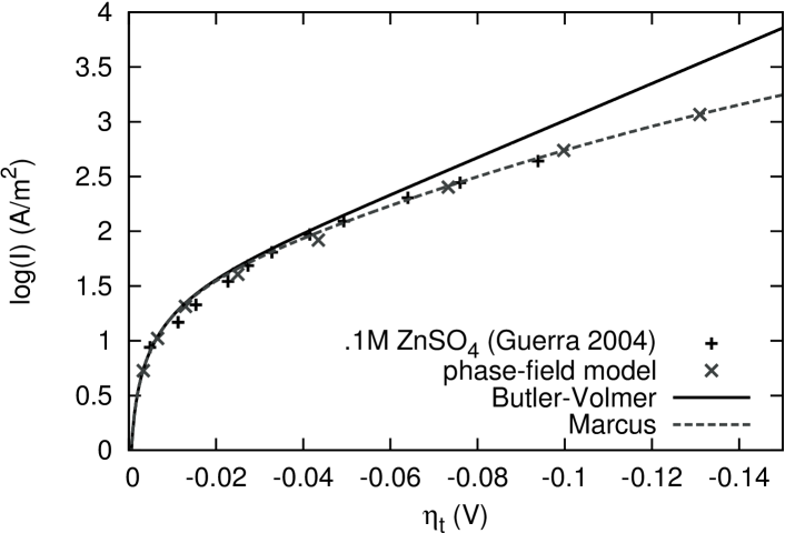
Figure 1: Tafel plot for zinc deposition from a 1.M ZnSO4 solution showing agreement between the phase-field model with an interfacial width of $1\,\mathrm{\mu m}$, the sharp interface limit (Eq. 5, Marcus kinetics), and experimental observation Guerra et al. (2004).

(a) Da=.1

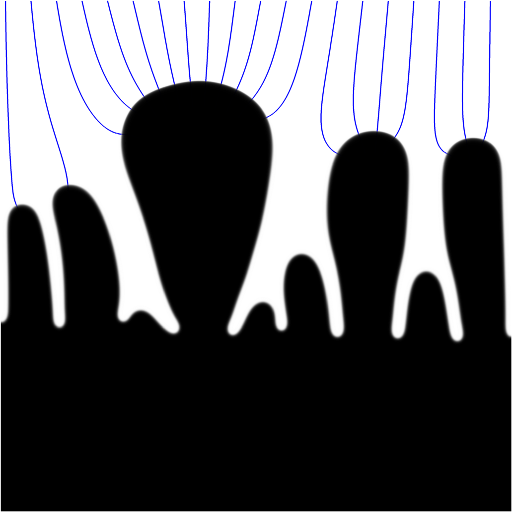
(b) Da=1

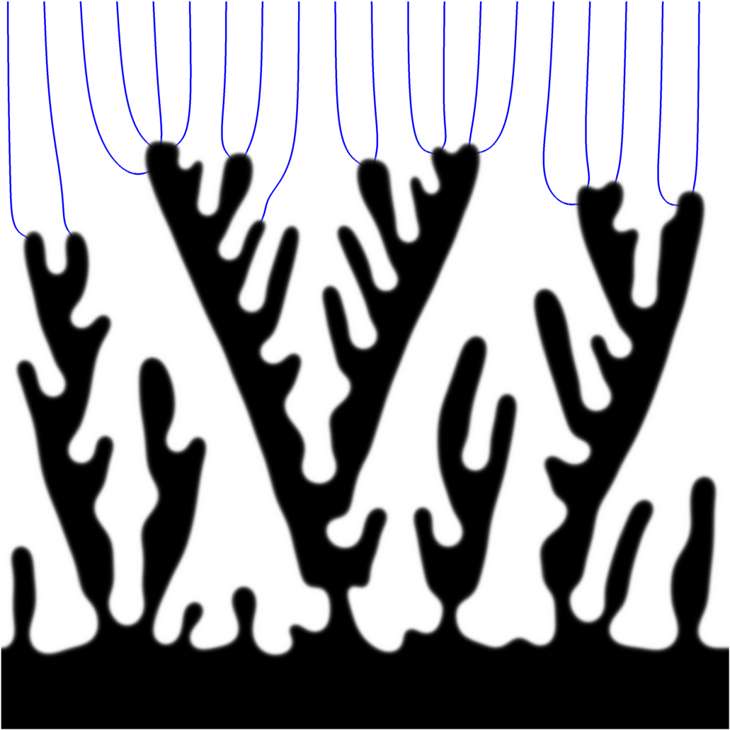
(c) Da=10

Figure 2: Simulated electrodeposition morphologies from a from a 1M ZnSO4 electrolyte at different Damkohler numbers. The width of each simulation is $150\,\mathrm{\mu m}$, and electric field lines are shown in blue.

Computation – The model was made non-variational by changing the interpolating function in Eq. 9 to $p(\xi)=\xi$ for numerical efficiency, and as required for the antitrapping current Karma and Rappel (1998); Karma (2001); Echebarria et al. (2004); Plapp (2011). Because zinc has a hexagonal crystal structure that strongly affects dendrite morphology Grier et al. (1986); Sawada et al. (1986), six-fold anisotropy in the interfacial energy was implemented using the standard approach Kobayashi (1993) with $\gamma(\theta)=\gamma\left[1+\epsilon_{6}\cos(6\theta)\right]$, where $\theta$ is the angle between the surface normal and the crystallographic axes, and $\epsilon_{6}=.01$ sets the strength of the anisotropy. The evolution equations (Eq. 7, 9, and 10) were solved using multigrid techniques detailed in Supplemental Material. Other simulation parameters are presented in Table 1.

The model was parameterized in terms of a dimensionless Damkohler number, which expresses the relative importance of the reaction rate to diffusion, $Da=\frac{i_{0}V_{m}/n\mathcal{F}}{D/L}$, where $i_{0}$ is the exchange current density, $n$ the number of electrons transferred, $D$ the electrolyte diffusivity, and $L$ the distance between the two electrodes. 2D simulations were performed for direct comparison with experimental morphologies obtained from 2D thin-cell geometries.

Results – Fig. 1 shows the success of the phase-field model at reproducing Marcus kinetics while addressing the length scale challenge. The interface was widened by roughly three orders of magnitude to $1\,\mathrm{\mu m}$, yet the underlying nonlinear kinetics occurring at the scale of the electric double layer were accurately reproduced.

Fig. 2 examines the effect of the Damkohler number on dendrite growth morphology, revealing that low Damkohler numbers have a dramatic effect on suppressing the formation of dendrites. Reaching a kinetically limited regime before reaching a transport-limited regime is like imposing a speed limit on the velocity of the interface, lessening the disparate interface velocities that lead to dendrites. Dendrites grow when the electric field concentrates at protrusions, increasing the local overpotential and enhancing growth. As dendrites grow taller they attract more electric field lines and screen their shorter neighbors, whose growth eventually ceases (see video in Supplemental Material).

Surface energy anisotropy plays an important role in growth morphology as well Grier et al. (1986). Zinc has a hexagonal crystal structure and tends to grow branching or fractal dendrites, while lithium, with a cubic crystal structure (less inherent anisotropy), grows needle-like dendrites. Simulation with 4-fold anisotropy indeed produces needles (see Supplemental Material).

In the diffusion limited regime, fractal dimension has proved to be a reliable measure for electrodeposits, with that of zinc consistently measured in the range 1.60-1.75 Grier et al. (1986); Argoul et al. (1988); Kahanda and Tomkiewicz (1989); Trigueros et al. (1991). Using the box counting method Karperien (2013), the fractal dimension of Fig. 2 (c) was found to be 1.67, showing the capability of the phase-field model to capture fractal growth phenomena.

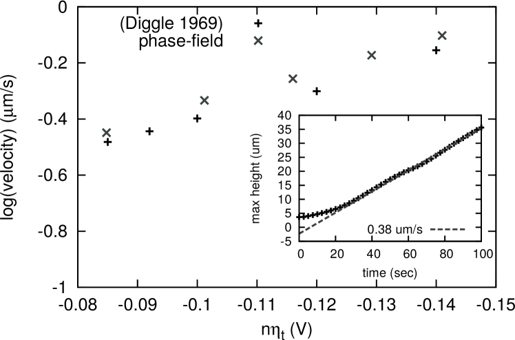
Figure 3: Comparison of simulated and experimental dendrite tip velocity as a function of overpotential for deposition of zinc from a $1.\mathrm{M}$ zincate electrolyte. An exchange current of $i_{0}=1000\,\mathrm{A/m^{2}}$ was used for zincate, following Diggle et al. (1969), and $Da=10$. The inset figure shows the hight of a simulated dendrite tip ($n\eta_{t}=84\,\mathrm{mV}$) with time.

After an initial formation stage, zinc dendrite tips are observed to grow at a constant velocity that depends exponentially on the applied overpotential Diggle et al. (1969). Fig. 3 shows agreement between experimental tip velocity measurements and phase-field simulations of single dendrites grown from a perturbation. The inset figure shows the height of a simulated dendrite vs time, revealing that the dendrite grew at constant velocity. Since the velocity $v$ is proportional to the tip current, a linear relationship between $\log(v)$ and $\eta_{t}$ exists, as shown in Fig. 3, with the expected Tafel slope of $\alpha=.5$.

Zinc dendrite tips are also know to be a parabolic with a characteristic radius of curvature Diggle et al. (1969). The simulations in Fig. 3 produced parabolic tips with curvatures ranging from $85.\mathrm{\mu m}$ to $1.15\,\mathrm{\mu m}$, within the rage measured by Diggle et al. Diggle et al. (1969) (see Table VIII). Details of how the curvature was measured are in Supplemental Material. Importantly, tip curvature cannot be predicted from models such as DLA that do not account for surface energy.

Discussion – Preventing dendrite growth by improving electrolyte transport in batteries (the denominator of the Damkohler number) has been demonstrated recently Park et al. (2014), but little effort has been spent targeting the exchange current, despite the fact that kinetics are known to vary by orders of magnitude with slight changes in electrolyte composition Bard (1973). Surprisingly, reducing the exchange current to smoothen deposits appears to have been reported in a different context for cadmium decades ago Sotnikova and Loshkarev (1950), and may also explain why magnesium, with an exchange current orders of magnitude smaller than lithium or zinc Peled and Straze (1977), is not observed to grow dendrites Matsui (2011). Recently it was observed that a small amount of bismuth at zinc surface inhibits dendrite growth Gallaway et al. (2014), which might also be related to reaction kinetics.

Finally, there appear to be many similarities between electrodeposition and the phenomenon of viscous fingering Homsy (1987). In addition to visually similar morphologies, the growth process of both occur via mechanisms of shielding, spreading, and tip splitting. The exchange current in electrodeposition appears to act as a stabilizing force in an analogous way to gravitational stabilization of viscous fingering.

In conclusion, a phase-field model of electrochemical interfaces was developed to study the growth of dendrites during electrodeposition. The model was derived in the grand canonical ensemble to allow the interface to be widened to simulate experimental length and time scales, and Faradaic reactions were modeled rigorously with Marcus kinetics. Damkohler number, overpotential, and electrolyte concentration were investigated, and the model accurately reproduced the reaction kinetics, fractal dimension, and tip velocity and curvature of zinc dendrites. The results suggest that engineering the electrolyte to decrease the reaction kinetics could be a successful strategy for controlling dendrite growth.