Optimizing The Integrator Step Size for Hamiltonian Monte Carlo

Abstract

Hamiltonian Monte Carlo can provide powerful inference in complex statistical problems, but ultimately its performance is sensitive to various tuning parameters. In this paper we use the underlying geometry of Hamiltonian Monte Carlo to construct a universal optimization criterion for tuning the step size of the symplectic integrator crucial to any implementation of the algorithm as well as diagnostics to monitor for any signs of invalidity. An immediate outcome of this result is that the suggested target average acceptance probability of 0.651 can be relaxed to $0.6\lesssim a\lesssim 0.9$ with larger values more robust in practice.

journalname

, , and

Hamiltonian Monte Carlo (Duane et al., 1987; Neal, 2011; Betancourt et al., 2014) yields efficient inference that scales to high-dimensional problems by building up Markov transitions from a smooth maps known as Hamiltonian flow. In practice this flow must simulated by a numerical integrator and, while any bias can be corrected by applying a Metropolis acceptance procedure, the performance of the resulting algorithm is highly sensitive to the choice of integrator step size.

At present the integrator step size is typically set by applying the analysis in Beskos et al. (2013), which derived a lower bound for the cost of the algorithm as a function of the integrator step size when targeting an independently and identically distributed target distribution and a second-order leapfrog integrator. In this paper we build upon that work, introducing a complementary upper bound that admits a more robust optimization criterion for the integrator step size and leveraging the geometry inherent to the algorithm to extend the criterion to any target distribution and any symplectic integrator.

In order to build such an optimization criterion we first relate the computational cost of a Hamiltonian Monte Carlo transition to various expectations that depend on the integrator and the chosen step size. We next show how to approximate these expectations and then use those results to construct a robust optimization criterion by minimizing the cost. Finally, we discuss how those approximations may fail in practice and how to compensate the optimization procedure to ensure robust application.

1 Bounding The Cost of a Hamiltonian Monte Carlo Transition

Hamiltonian Monte Carlo transitions are generated from a Hamiltonian,

$$H\!\left(q,p\right)=T\!\left(q,p\right)+V\!\left(q\right),$$

where the kinetic energy, $T\!\left(q,p\right)$, is specified by the user subject to certain constraints (Betancourt et al., 2014, Sec. 3.1.3) and the potential energy is defined by a given target distribution, $V\!\left(q\right)=-\log\varpi\!\left(q\right)$. Beginning with an initial position, $q$, each transition generates a joint state by randomly sampling the momenta,

$$p\sim\varpi_{q}\!\left(p|q\right)\propto\exp\!\left(-T\!\left(q,p\right)\right),$$

and then producing a new state by integrating Hamilton’s equations,

$$\frac{dq}{dt} =+\frac{\partial H}{\partial p}=+\frac{\partial T}{\partial p}$$

$$\frac{dp}{dt} =-\frac{\partial H}{\partial q}=-\frac{\partial T}{\partial q}-\frac{\partial V}{\partial q}.$$

for some time $\tau$.

When Hamilton’s equations are integrated exactly the joint state is distributed as

$$\left(q,p\right)\sim\varpi_{H}\!\left(q,p\right)\propto\exp\!\left(-H\!\left(q,p\right)\right)$$

while the position is marginally distributed according to the desired target distribution,

$$q\sim\varpi\!\left(q\right).$$

In practice, however, the Hamiltonian trajectory can be integrated only approximately and the stationary distribution of the position will be biased away from $\varpi$.

If we use a $k$th-order symmetric symplectic integrator with step size $\epsilon$ to simulate the Hamiltonian trajectory, then we can exactly cancel this bias with a straightforward Metropolis scheme. First we compose the approximate Hamiltonian trajectory, $\phi^{\tilde{H}}_{\epsilon,\tau}\!\left(q,p\right)$, with a momentum reversal operator, $R:\left(q,p\right)\mapsto\left(q,-p\right)$, to generate a proposal,

$$\Phi^{\tilde{H}}_{\epsilon,\tau}\!\left(q,p\right)=R\circ\phi^{\tilde{H}}_{\epsilon,\tau}\!\left(q,p\right).$$

This proposal is then accepted only with the probability,

$$a\!\left(q,p\right)=\min\!\left(1,\exp\!\left(\Delta_{\epsilon}\!\left(q,p\right)\right)\right),$$

where $\Delta_{\epsilon}\!\left(q,p\right)$ is the Hamiltonian error,

$$\Delta_{\epsilon}\!\left(q,p\right)=-H\circ\Phi^{\tilde{H}}_{\epsilon,\tau}\!\left(q,p\right)+H\!\left(q,p\right).$$

The number of attempts required to produce an accepted proposal follows a geometric distribution with the probability of success

$$a\!\left(q\right)=\mathbb{E}_{\varpi_{q}}\!\left[a\!\left(q,p\right)\right].$$

With the cost of generating a proposal just the cost of simulating at trajectory,

$$C_{\mathrm{proposal}}=C_{\mathrm{iteration}}\frac{\tau}{\epsilon},$$

the expected cost of generating an accepted proposal is given by averaging the expected number of rejections over the position space,

$$\mathbb{E}_{q}\!\left[C\right]=\mathbb{E}_{\varpi}\!\left[C_{\mathrm{proposal}}\,r\right]\\ =\frac{C_{\mathrm{iteration}}}{\epsilon}\mathbb{E}_{\varpi}\!\left[\tau\,r\right].$$

If $\tau$ is chosen independently of position, then

$$\mathbb{E}_{q}\!\left[C\right] =C_{\mathrm{iteration}}\frac{\tau}{\epsilon}\cdot\mathbb{E}_{\varpi}\left[\frac{1}{a\!\left(q\right)}\right]$$

$$=C_{\mathrm{iteration}}\frac{\tau}{\epsilon}\cdot\mathbb{E}_{\varpi}\left[\frac{1}{\mathbb{E}_{\varpi_{q}}\left[a\!\left(q,p\right)\right]}\right].$$

Following Beskos et al. (2013, Eq. 4.2), we apply Jensen’s inequality to the outer expectation to yield a lower bound on the expected cost. Jensen’s inequality, however, can also be applied on the inner expectation to give a complementary upper bound,

$$\frac{1}{\mathbb{E}_{\varpi_{H}}\left[a\!\left(q,p\right)\right]}\leq\mathbb{E}_{\varpi}\left[\frac{1}{\mathbb{E}_{\varpi_{q}}\left[a\!\left(q,p\right)\right]}\right]\leq\mathbb{E}_{\varpi_{H}}\left[\frac{1}{a\!\left(q,p\right)}\right].$$ (1)

These bounds are particularly advantageous because they reduce to expectations of functions of the error in the Hamiltonian, $\Delta_{\epsilon}\!\left(q,p\right)$, with respect to the joint distribution, $\varpi_{H}$. These expectations admit well-behaved approximations independent of the actual form of the potential and kinetic energies and hence the particular details of the given problem.

2 Approximating Canonical Expectations

More formally, expectations with respect to the joint distribution, $\varpi_{H}$, in Hamiltonian Monte Carlo are canonical expectations and are readily estimated in practice with symplectic integrators. In this section we define canonical expectations and their relationship to Hamiltonian Monte Carlo, show how symplectic integrators approximate these canonical expectations and constrain the accuracy of these approximations in general, and then ultimately construct universal approximations to canonical expectations of certain functions of the Hamiltonian error.

This construction is necessarily technical and requires a strong familiarity with differential geometry and the geometric foundations of Hamiltonian Monte Carlo (Betancourt et al., 2014). We reserve the detailed proofs to Appendix A and suggest that readers interested in only the final result skip ahead to Section 3.

2.1 Canonical Expecations

Hamiltonian systems, $\left(M,\omega,H\right)$, where $M$ is a smooth, $2n$-dimensional manifold, $\omega$ a symplectic form, and $H:M\rightarrow\mathbb{R}$ a smooth function, are particularly rich probabilistic systems. In the following we review how probability measures arise naturally on Hamiltonian systems, the implicit Hamiltonian system and corresponding measures driving Hamiltonian Monte Carlo, and how expectations with respect to such measures can be computed in theory.

2.1.1 Canonical Distributions and Expectations

On a Hamiltonian system the symplectic form, $\omega$, immediately defines a canonical volume form,

$$\Omega=\wedge_{i=1}^{n}\omega,$$

or, in canonical coordinates,

$$\Omega =\mathrm{d}q^{1}\wedge\ldots\wedge\mathrm{d}q^{n}\wedge\mathrm{d}p_{1}\wedge\ldots\wedge\mathrm{d}p_{n}.$$

Provided that $\int_{M}e^{-\beta H}\Omega$ is finite for some $\beta\in\mathbb{R}$, we can also construct canonical probability measures,

$$\varpi_{H}=\frac{e^{-\beta H}\Omega}{\int_{M}e^{-\beta H}\Omega},$$

known as canonical distributions. We refer to expectations of functions with respect to canonical distributions as canonical expectations.

The Hamiltonian foliates the manifold, $M$, into level sets,

$$H^{-1}\!\left(E\right)=\left\{z\in M\,|\,H\!\left(z\right)=E\right\},$$

and $\varpi$ naturally disintegrates into microcanonical distristributions, $\pi_{H^{-1}(E)}$, that concentrate on these submanifolds,

$$\varpi_{H} =H^{*}\varpi_{E}\wedge\varpi_{H^{-1}\left(E\right)}$$

$$=\frac{e^{-\beta E}}{\int_{M}e^{-\beta H}\Omega}d\!\left(E\right)\mathrm{d}E\wedge\frac{\vec{v}\,\lrcorner\,\Omega}{d\!\left(E\right)}.$$

Here $\vec{v}$ is any transverse vector field satisfying $\mathrm{d}H\!\left(\vec{v}\right)=c$, $\iota_{E}:H^{-1}\!\left(E\right)\hookrightarrow M$ is the inclusion of $H^{-1}\!\left(E\right)$ into $M$, and

$$d\!\left(E\right)=\frac{\int_{H^{-1}\left(E\right)}\iota^{*}_{E}\!\left(\vec{v}\,\lrcorner\,\Omega\right)}{\mathrm{d}H\!\left(v\right)}.$$

is the density of states. Without loss of generality we will always rescale $\vec{v}$ such that $\mathrm{d}H\!\left(\vec{v}\right)=1$.

Combined with the symplectic form, the Hamiltonian also generates a Hamiltonian flow,

$$\phi^{H}_{t}:M\rightarrow M,\,t\in\mathbb{R},$$

under which both the symplectic volume form and Hamiltonian, and consequently the canonical and microcanonical distributions, are invariant.

2.1.2 Hamiltonian Monte Carlo and Canonical Expectations

Because it preserves the canonical distribution, Hamiltonian flow can be used to construct an efficient Markov transition. The only problem is that a given probability space, $\left(Q,\mathcal{B}\!\left(Q\right),\varpi\right)$, does not have the symplectic structure necessary be a Hamiltonian system.

Hamiltonian Monte Carlo leverages Hamiltonian flow by considering not the sample space, $Q$, but rather it’s cotangent bundle, $T^{*}Q$. If $Q$ is a smooth and orientable $n$-dimensional manifold then the cotangent bundle is itself a smooth, orientable $2n$-dimensional manifold with a canonical fiber bundle structure, $\pi:T^{*}Q\rightarrow Q$, and a canonical symplectic form, $\omega$.

The target measure on $Q$, given in canonical coordinates by

$$\varpi\propto e^{-V}\mathrm{d}q^{1}\wedge\ldots\wedge\mathrm{d}q^{n},$$

is lifted onto the cotangent bundle with the choice of a disintegration,

$$\varpi_{q}\propto e^{-T}\mathrm{d}p_{1}\wedge\ldots\wedge\mathrm{d}p_{n}+\text{horizontal}\;n\text{-forms},$$

yielding the joint measure

$$\varpi_{H} =\pi^{*}\varpi_{q}\wedge\varpi$$

$$\propto e^{-T-V}\mathrm{d}p_{1}\wedge\ldots\wedge\mathrm{d}p_{n}\wedge\mathrm{d}q^{1}\wedge\ldots\wedge\mathrm{d}q^{n}$$

$$\propto e^{-\left(T+V\right)}\Omega.$$

Taking,

$$H=-\log\frac{\mathrm{d}\varpi_{H}}{\mathrm{d}\Omega}=T+V,$$

this lift defines a Hamiltonian system, $\left(T^{*}Q,\omega,H\right)$, where the joint measure $\varpi_{H}$ is exactly the unit canonical measure with $\beta=1$. In particular, expectations with respect to $\varpi_{H}$ are all canonical expectations.

2.1.3 Computing Canonical Expectations

One of the important benefits of a Hamiltonian system is that the canonical expectation of any smooth function, $f:M\rightarrow\mathbb{R}$, with respect to the canonical distribution

$$\mathbb{E}_{\varpi_{H}}\!\left[f\right]=\int_{M}f\,\varpi_{H}=\frac{\int_{M}fe^{-\beta H}\Omega}{\int_{M}e^{-\beta H}\Omega},$$

can be computed by taking expectations with respect to the microcanonical distributions on the level sets,

$$\mathbb{E}_{\varpi_{H}}\!\left[f\right] =\int_{M}f\,\varpi_{H}$$

$$=\int_{M}\varpi_{H^{-1}\left(E\right)}\wedge\varpi_{E}$$

$$=\frac{1}{\int_{M}e^{-\beta H}\Omega}\int\mathrm{d}E\,d\!\left(E\right)e^{-\beta E}\frac{\int_{H^{-1}\left(E\right)}\iota^{*}_{E}\!\left(f\,\vec{v}\,\lrcorner\,\Omega\right)}{d\!\left(E\right)}.$$

In particular the microcanonical expectations are readily computed using the Hamiltonian flow. Birkhoff’s ergodic theorem (Petersen, 1989) states that given certain ergodicity conditions the expectation of any function with respect to the microcanonical distribution is equal to its expectation along the Hamiltonian flow,

$$\frac{\int_{H^{-1}\left(E\right)}\iota^{*}_{E}\!\left(f\,\vec{v}\,\lrcorner\,\Omega\right)}{d\!\left(E\right)} =\lim_{T\rightarrow\infty}\frac{1}{T}\int_{0}^{T}\mathrm{d}t\,\left(\phi^{H}_{t}\right)^{*}f$$

$$\equiv\left<f\right>_{H^{-1}\left(E\right)}.$$

2.2 Approximating Canonical Expectations with Symplectic Integrators

The only problem with using Hamiltonian flow to compute expectations is that the Hamiltonian flow itself requires the solution to a system of $2n$ first-order ordinary differential equations. For all but the simplest systems, analytical solution are unfeasible and we must instead resort to simulating the flow numerically.

Fortunately, there exist a family of numerical integrators that leverage the underlying symplectic geometry to conserve many of the properties of the exact flow (Hairer, Lubich and Wanner, 2006; Leimkuhler and Reich, 2004). These symplectic integrators exactly preserve the symplectic volume form with only small variations in the Hamiltonian along the simulated flow.

In fact, symplectic integrators simulate some flow exactly, just not the flow corresponding to $H$. Using backwards error analysis one can show that a $k$-th order symmetric symplectic integrator exactly simulates the flow for some modified Hamiltonian, given by an even, asymptotic expansion with respect to the integrator step size, $\epsilon$,

$$\widetilde{H}=H+\sum_{n=k/2}^{N}\epsilon^{2n}H_{\left(n\right)}+\mathcal{O}\!\left(e^{-c/\epsilon}\right).$$

Because it is exponentially small in the step size, the asymptotic error is typically neglected and the leading-order behavior of is given by

$$\widetilde{H}=H+\epsilon^{k}G+\mathcal{O}(\epsilon^{k+2}).$$

As in the exact case, the modified Hamiltonian foliates the manifold and we can define level sets,

$$\widetilde{H}^{-1}\!\left(E\right)=\left\{z\in M\,|\,\widetilde{H}\!\left(z\right)=E\right\},$$

a corresponding inclusion map,

$$\tilde{\iota}_{E}:\widetilde{H}^{-1}\!\left(E\right)\hookrightarrow M,$$

and a corresponding transverse vector field,

$$\mathrm{d}\widetilde{H}\!\left(\vec{u}\right)=1.$$

Provided that the asymptotic error is indeed negligible and the symplectic integrator is topologically stable (McLachlan, Perlmutter and Quispel, 2004), the modified level sets will have the same topology as the exact level sets. In particular, when the exact foliation defines a well-behaved disintegration into microcanonical distributions we can define a corresponding modified density of states,

$$\tilde{d}\!\left(E\right)=\int_{\widetilde{H}^{-1}\left(E\right)}\tilde{\iota}^{*}_{E}\!\left(\vec{u}\,\lrcorner\,\Omega\right),$$

modified microcanonical distribution,

$$\varpi_{\widetilde{H}^{-1}\left(E\right)}=\frac{\vec{u}\,\lrcorner\,\Omega}{\tilde{d}\!\left(E\right)},$$

and modified canonical distribution,

$$\varpi_{\tilde{H}} =\tilde{H}^{*}\widetilde{\varpi}_{E}\wedge\varpi_{\widetilde{H}^{-1}\left(E\right)}$$

$$=\frac{e^{-\beta E}}{\int_{M}e^{-\beta\widetilde{H}}\Omega}\tilde{d}\!\left(E\right)\mathrm{d}E\wedge\frac{\vec{u}\,\lrcorner\,\Omega}{\tilde{d}\!\left(E\right)}.$$

Using the flow from a numerical integrator to compute averages yields expectations with respect to these modified measures,

$$\mathbb{E}_{\varpi_{\widetilde{H}}}\!\left[f\right] =\int_{M}f\,\varpi_{\widetilde{H}}$$

$$=\frac{1}{\int_{M}e^{-\beta\widetilde{H}}\Omega}\int\mathrm{d}E\,\tilde{d}\!\left(E\right)e^{-E}\frac{\int_{\widetilde{H}^{-1}\left(E\right)}\tilde{\iota}^{*}_{E}\!\left(f\,\vec{u}\,\lrcorner\,\Omega\right)}{\tilde{d}\!\left(E\right)},$$

where

$$\frac{\int_{\widetilde{H}^{-1}\left(E\right)}\tilde{\iota}^{*}_{E}\!\left(f\,\vec{u}\,\lrcorner\,\Omega\right)}{\tilde{d}\!\left(E\right)} =\lim_{T\rightarrow\infty}\frac{1}{T}\int_{0}^{T}\mathrm{d}t\,\left(\phi^{\widetilde{H}}_{t}\right)^{*}f$$

$$\equiv\left<f\right>_{\widetilde{H}^{-1}\left(E\right)}.$$

The ultimate utility of a symplectic integrator and its modified Hamiltonian system is in the accuracy of its expectations relative to the true canonical expectations. Fortunately, the geometric structure of symplectic integrators ensures that the approximation error of both microcanonical and canonical expectations computed with a symplectic integrator is well-controlled.

Theorem 1.

Let $\left(M,\omega,H\right)$ be a Hamiltonian system and consider a $k$-th order symmetric symplectic integrator with the corresponding modified Hamiltonian $\widetilde{H}=H+\epsilon^{k}\,G+\mathcal{O}(\epsilon^{k+2})$. If the integrator is topologically stable and the asymptotic error is negligible, then the difference in the microcanonical and modified microcanonical expectations for any smooth function, $f:M\rightarrow\mathbb{R}$, is given by

$$\left<f\right>_{H^{-1}\left(E\right)}-\left<f\right>_{\widetilde{H}^{-1}\left(E\right)}= +\epsilon^{k}\left<f\,\mathrm{d}G\!\left(\vec{v}\right)+G\,\mathrm{d}f\!\left(\vec{v}\right)+f\,G\left(\frac{\partial v^{i}}{\partial q^{i}}+\frac{\partial v_{i}}{\partial p_{i}}\right)\right>_{\widetilde{H}^{-1}\left(E\right)}$$

$$-\epsilon^{k}\Big{<}f\Big{>}_{\widetilde{H}^{-1}\left(E\right)}\left<\mathrm{d}G\!\left(\vec{v}\right)+G\left(\frac{\partial v^{i}}{\partial q^{i}}+\frac{\partial v_{i}}{\partial p_{i}}\right)\right>_{\widetilde{H}^{-1}\left(E\right)}+\mathcal{O}(\epsilon^{k+2}),$$

where $\vec{v}$ is any transverse vector field satisfying $\mathrm{d}H\!\left(\vec{v}\right)=1$.

Note that, when $H^{-1}\!\left(E\right)$ and $\widetilde{H}^{-1}\!\left(E\right)$ intersect at some initial point, this reduces to the calculation in Arizumi and Bond (2012). Moreover, to leading-order we can replace to the expectations over $\widetilde{H}^{-1}\!\left(E\right)$ on the RHS with expectations over $H^{-1}\!\left(E\right)$ to give

$$\left<f\right>_{H^{-1}\left(E\right)}-\left<f\right>_{\widetilde{H}^{-1}\left(E\right)}= +\epsilon^{k}\left<f\,\mathrm{d}G\!\left(\vec{v}\right)+G\,\mathrm{d}f\!\left(\vec{v}\right)+f\,G\left(\frac{\partial v^{i}}{\partial q^{i}}+\frac{\partial v_{i}}{\partial p_{i}}\right)\right>_{H^{-1}\left(E\right)}$$

$$-\epsilon^{k}\left<f\right>_{H^{-1}\left(E\right)}\left<\mathrm{d}G\!\left(\vec{v}\right)+G\left(\frac{\partial v^{i}}{\partial q^{i}}+\frac{\partial v_{i}}{\partial p_{i}}\right)\right>_{H^{-1}\left(E\right)}+\mathcal{O}(\epsilon^{k+2}).$$

This is convenient for numerical experiments when the canonical expectations can be computed analytically.

Given the decomposition of the canonical distributions over level sets, the result for the accuracy of microcanonical expectations immediately carries over to a canonical expectations.

Theorem 2.

Let $\left(M,\omega,H\right)$ be a Hamiltonian system and consider a $k$-th order symmetric symplectic integrator with the corresponding modified Hamiltonian $\widetilde{H}=H+\epsilon^{k}\,G+\mathcal{O}(\epsilon^{k+2})$. If the integrator is topologically stable and the asymptotic error is negligible, then the difference in the canonical and modified canonical expectations for any smooth function, $f:M\rightarrow\mathbb{R}$, is given by

$$\mathbb{E}_{\varpi_{H}}\!\left[f\right]-\mathbb{E}_{\varpi_{\widetilde{H}}}\!\left[f\right]= +\epsilon^{k}\,\mathbb{E}_{\varpi_{H}}\!\left[f\,\mathrm{d}G\!\left(\vec{v}\right)+G\,\mathrm{d}f\!\left(\vec{v}\right)+f\,G\left(\frac{\partial v^{i}}{\partial q^{i}}+\frac{\partial v_{i}}{\partial p_{i}}\right)\right]$$

$$-\epsilon^{k}\,\mathbb{E}_{\varpi_{H}}\!\left[f\right]\,\mathbb{E}_{\varpi_{H}}\!\left[\mathrm{d}G\!\left(\vec{v}\right)+G\left(\frac{\partial v^{i}}{\partial q^{i}}+\frac{\partial v_{i}}{\partial p_{i}}\right)\right]+\mathcal{O}(\epsilon^{k+2}),$$

where $\vec{v}$ is any transverse vector field satisfying $\mathrm{d}H\!\left(\vec{v}\right)=1$.

2.3 Approximating Canonical Expectations of the Hamiltonian Error

The expectations necessary for bounding the cost of a basic Hamiltonian Monte Carlo transition are not just any canonical expectations but canonical expectations of functions of the Hamiltonian error,

$$\Delta_{\epsilon}=H-H\circ\Phi^{\widetilde{H}}_{\epsilon,\tau},$$

where again

$$\Phi^{\widetilde{H}}_{\epsilon,\tau}=R\circ\phi^{\widetilde{H}}_{\epsilon,\tau}$$

is the Metropolis proposal. By constraining how the moments and then the cumulants of the Hamiltonian error scale with the symplectic integrator step size we can construct universal approximations to these particular expectations.

2.3.1 Moments of the Hamiltonian Error

Lemma 3.

Let $\left(M,\omega,H\right)$ be a Hamiltonian system and consider a $k$-th order symmetric symplectic integrator with the corresponding modified Hamiltonian $\widetilde{H}=H+\epsilon^{k}\,G+\mathcal{O}(\epsilon^{k+2})$ and Metropolis proposal $\Phi^{\widetilde{H}}_{\epsilon,\tau}$. If the integrator is topologically stable and the asymptotic error is negligible, then the moments of the Hamiltonian error with respect to the unit canonical distribution scale as

$$\mathbb{E}_{\varpi_{H}}\!\left[\left(\Delta_{\epsilon}\right)^{n}\right]\propto\left\{\begin{array}[]{rr}\epsilon^{k(n+1)},&n\,\mathrm{odd}\\ \epsilon^{kn}\;\,,&n\,\mathrm{even}\end{array}\right..$$

to leading-order in $\epsilon$.

The mean of the Hamiltonian error is particularly interesting because it can be computed analytically (Appendix A.3). In the case of a Gaussian target distribution, a Euclidean kinetic energy, and a second-order leapfrog integrator we have the Hamiltonian,

$$H=\frac{1}{2}p^{2}+\frac{1}{2}q^{2},$$

the sub-leading contribution to the modified Hamiltonian,

$$G=\frac{1}{24}\left(2q^{2}-p^{2}\right),$$

and eventually the average error

$$\mathbb{E}_{\varpi_{H}}\left[\Delta_{\epsilon}\right] =\frac{1}{64}\epsilon^{4}\left(1-\cos 2\tau\right)+\mathcal{O}\!\left(\epsilon^{6}\right),$$

in agreement with numerical experiments (Figure 1).

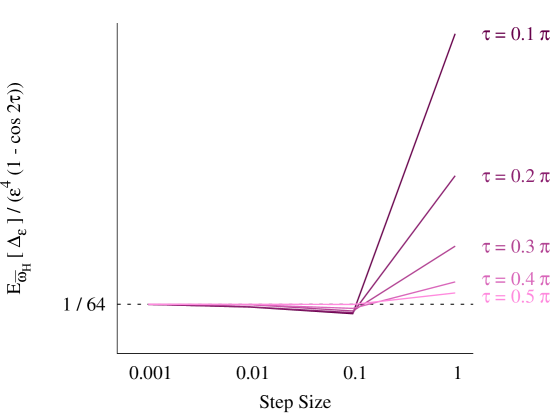
Figure 1: For the Gaussian target distribution, numerical estimates of $\mathbb{E}_{\varpi_{H}}\left[\Delta_{\epsilon}\right]$ are consistent with the geometric results for a wide range of integration times, $\tau$, and step sizes, $\epsilon$, at least until higher-order contributions become significant at large step sizes. The estimates were performed using an analytic form of the error such that discretization of the integration time is not a factor at larger step sizes.

2.3.2 Cumulants of the Hamiltonian Error

Lemma 4.

Let $\left(M,\omega,H\right)$ be a Hamiltonian system and consider a $k$-th order symmetric symplectic integrator with the corresponding modified Hamiltonian $\widetilde{H}=H+\epsilon^{k}\,G+\mathcal{O}(\epsilon^{k+2})$ and Metropolis proposal $\Phi^{\widetilde{H}}_{\epsilon,\tau}$. If the integrator is topologically stable and the asymptotic error is negligible, then the cumulants of the Hamiltonian error with respect to the unit canonical distribution scale as

$$\kappa_{n}\!\left(\Delta_{\epsilon}\right)\propto\left\{\begin{array}[]{rr}\epsilon^{k(n+1)},&n\,\mathrm{odd}\\ \epsilon^{kn}\;\,,&n\,\mathrm{even}\end{array}\right..$$

to leading-order in $\epsilon$.

Lemma 5.

Let $\left(M,\omega,H\right)$ be a Hamiltonian system and consider a $k$-th order symmetric symplectic integrator with the corresponding modified Hamiltonian $\widetilde{H}=H+\epsilon^{k}\,G+\mathcal{O}(\epsilon^{k+2})$ and Metropolis proposal $\Phi^{\widetilde{H}}_{\epsilon,\tau}$. If the integrator is topologically stable and the asymptotic error is negligible, then the cumulant generating function of the Hamiltonian error vanishes

$$\log\mathbb{E}_{\varpi_{H}}\!\left[e^{\Delta_{\epsilon}}\right]=0.$$

for the unit canonical distribution,

$$\varpi_{H}=\frac{e^{-H}\Omega}{\int_{M}e^{-H}\Omega}.$$

When coupled with Jensen’s inequality, Lemma 5 implies that $\mathbb{E}_{\varpi_{H}}\!\left[\Delta_{\epsilon}\right]\leq 0$ with equality holding only for an exact integrator when $\Delta_{\epsilon}$ is identically zero. This shows that a symplectic integrator will always introduce an error in expectation and the average Metropolis acceptance probability will always be smaller than unity.

Corollary 6.

Let $\left(M,\omega,H\right)$ be a Hamiltonian system and consider a $k$-th order symmetric symplectic integrator with the corresponding modified Hamiltonian $\widetilde{H}=H+\epsilon^{k}\,G+\mathcal{O}(\epsilon^{2k})$ and Metropolis proposal $\Phi^{\widetilde{H}}_{\epsilon,\tau}$. If the integrator is topologically stable and the asymptotic error is negligible, then to leading-order in $\epsilon$ the first two cumulants of the unit canonical distribution satisfy

$$\kappa_{1}=-\frac{1}{2}\kappa_{2}.$$

Proof.

The cumulant generating function gives

$$\log\mathbb{E}_{\varpi_{H}}\left[e^{t\Delta_{\epsilon}}\right]=\sum_{n=0}^{\infty}\frac{t^{n}\kappa_{n}}{n!},$$

or taking $t=1$ and appealing to Lemma 5,

$$0=\log\mathbb{E}_{\varpi_{H}}\left[e^{\Delta_{\epsilon}}\right]=\sum_{n=0}^{\infty}\frac{\kappa_{n}}{n!},$$

But from Lemma 4 we know that to leading-order only the first two cumulants contribute,

$$0=\kappa_{1}+\frac{1}{2}\kappa_{2}+\mathcal{O}(\epsilon^{2k}),$$

or

$$\kappa_{1}=-\frac{1}{2}\kappa_{2}+\mathcal{O}(\epsilon^{2k}),$$

as desired.

∎

Explicitly introducing the scaling from Lemma 4 gives

$$\kappa_{2}\approx-2\kappa_{1}=\alpha\,\epsilon^{2k},\,\alpha\in\mathbb{R}.$$

At this point we can note that if the target distribution composes into $d$ independently and identically distributions components then the cumulants scale as

$$\kappa_{n}\!\left(\Delta_{\epsilon}\right)\propto\left\{\begin{array}[]{rr}d\,\epsilon^{k(n+1)},&n\,\mathrm{odd}\\ d\,\epsilon^{kn}\;\,,&n\,\mathrm{even}\end{array}\right..$$

If we scale the step size as $\epsilon^{2k}=\epsilon_{0}^{2k}/d$ then the cumulants scaling becomes

$$\kappa_{n}\!\left(\Delta_{\epsilon}\right)\propto\left\{\begin{array}[]{rr}d^{\frac{1-n}{2}}\,\epsilon_{0}^{k(n+1)},&n\,\mathrm{odd}\\ d^{\frac{2-n}{2}}\,\epsilon_{0}^{kn}\;\,,&n\,\mathrm{even}\end{array}\right..$$

Consequently, in the infinite limit $d\rightarrow\infty$ all of the cumulants beyond second-order vanish, $\varpi_{\Delta_{\epsilon}}$ converges to a $\mathcal{N}\!\left(-\frac{1}{2}\alpha\epsilon^{2k},\alpha\epsilon^{2k}\right)$ in distribution, and the desired expectations simply to Gaussian integrals. Extending this argument to independently but not necessarily identically distributed distributions corresponds to the results in Beskos et al. (2013) generalized to any symplectic integrator.

Fortunately, even outside of the limit of infinite independently distributed distributions the expectations are remarkably well-behaved.

2.3.3 Expectations of the Hamiltonian Error

Together, these Lemmas imply that canonical expectations of any smooth function of the Hamiltonian error, as well as the Metropolis acceptance probability with its single cusp, are well-approximated by straightforward Gaussian integrals.

Theorem 7.

Let $\left(M,\omega,H\right)$ be a Hamiltonian system and consider a $k$-th order symmetric symplectic integrator with the corresponding modified Hamiltonian $\widetilde{H}=H+\epsilon^{k}\,G+\mathcal{O}(\epsilon^{k+2})$ and Metropolis proposal $\Phi^{\widetilde{H}}_{\epsilon,\tau}$. If the integrator is topologically stable and the asymptotic error is negligible, then the expectation of any smooth function of the Hamiltonian error is given by

$$\mathbb{E}_{\varpi_{H}}\!\left[f\!\left(\Delta_{\epsilon}\right)\right] =\int^{\infty}_{-\infty}\mathrm{d}\Delta_{\epsilon}\,\mathcal{N}\!\left(\Delta_{\epsilon}|-\frac{1}{2}\alpha\,\epsilon^{2k},\alpha\,\epsilon^{2k}\right)f\!\left(\Delta_{\epsilon}\right)+\mathcal{O}(\epsilon^{2k+4}),$$

for some $\alpha\in\mathbb{R}$.

Theorem 8.

Let $\left(M,\omega,H\right)$ be a Hamiltonian system and consider a $k$-th order symmetric symplectic integrator with the corresponding modified Hamiltonian $\widetilde{H}=H+\epsilon^{k}\,G+\mathcal{O}(\epsilon^{k+2})$ and Metropolis proposal $\Phi^{\widetilde{H}}_{\epsilon,\tau}$. If the integrator is topologically stable and the asymptotic error is negligible, then the expectation of the Metropolis acceptance probability is given by

$$\mathbb{E}_{\varpi_{H}}\!\left[a\!\left(\Delta_{\epsilon}\right)\right]= \int^{\infty}_{-\infty}\mathrm{d}\Delta_{\epsilon}\,\mathcal{N}\!\left(\Delta_{\epsilon}|-\frac{1}{2}\alpha\,\epsilon^{2k},\alpha\,\epsilon^{2k}\right)a\!\left(\Delta_{\epsilon}\right)+\mathcal{O}(\epsilon^{k}),$$

for some $\alpha\in\mathbb{R}$.

3 Approximating Bounds and the Step Size Optimization Criterion

The approximation expectations in Theorem 7 and 8 immediately admit universal, approximation bounds on the cost of a basic Hamiltonian Monte Carlo transition, and minimizing these bounds provides a correspondingly universal strategy for tuning the integrator step size.

Theorem 9.

Provided that the symmetric symplectic integrator is topologically stable and the asymptotic error is negligible, the cost of a Hamiltonian Monte Carlo implementation with Metropolis proposal $\Phi^{\widetilde{H}}_{\epsilon,\tau}$ is bounded by functions of the average Metropolis acceptance probability, $a=\mathbb{E}_{\varpi_{H}}\left[a\!\left(q,p\right)\right]$,

$$\frac{1}{\epsilon\!\left(a\right)a}+\mathcal{O}(\epsilon^{k})\leq\frac{1}{\tau}\frac{\left<C\right>}{C_{\mathrm{iteration}}}\leq\frac{\frac{a}{2}+\Phi\!\left(-3\Phi^{-1}\!\left(a/2\right)\right)\exp\!\left(4\left(\Phi^{-1}\!\left(a/2\right)\right)^{2}\right)}{\epsilon\!\left(a\right)}+\mathcal{O}(\epsilon^{k}),$$

where

$$\epsilon\!\left(a\right)=\left[\sqrt{\frac{2}{\alpha}}\Phi^{-1}\!\left(1-\frac{a}{2}\right)\right]^{1/k}$$

for some $\alpha\in\mathbb{R}$.

Proof.

Approximations for the both the lower and upper bounds in (1) are given immediately by carrying out the Gaussian integrals analytically (Roberts, Gelman and Gilks, 1997),

$$\mathbb{E}_{\varpi_{H}}\left[a\!\left(q,p\right)\right] =2\,\Phi\!\left(-\sqrt{\frac{\alpha}{2}}\epsilon^{k}\right)+\mathcal{O}(\epsilon^{k})$$

$$\mathbb{E}_{\varpi_{H}}\left[1/a\!\left(q,p\right)\right] =\mathbb{E}_{\varpi_{H}}\left[1+e^{-\Delta_{\epsilon}}\right]-\mathbb{E}_{\varpi_{H}}\left[a\!\left(-\Delta_{\epsilon}\right)\right]$$

$$=\Phi\!\left(-\sqrt{\frac{\alpha}{2}}\epsilon^{k}\right)+\Phi\!\left(3\sqrt{\frac{\alpha}{2}}\epsilon^{k}\right)e^{2\,\alpha\,\epsilon^{2k}}+\mathcal{O}(\epsilon^{k}).$$

Following previous work (Roberts, Gelman and Gilks, 1997; Beskos et al., 2013) we now consider the cost as a function of not the step size but rather the average acceptance probability,

$$a\equiv\mathbb{E}_{\varpi_{H}}\left[a\!\left(q,p\right)\right]=2\,\Phi\!\left(-\sqrt{\frac{\alpha}{2}}\epsilon^{k}\right)+\mathcal{O}(\epsilon^{k}),$$ (2)

Solving for the step size yields

$$\epsilon\!\left(a\right)=\left[\sqrt{\frac{2}{\alpha}}\Phi^{-1}\!\left(1-\frac{a}{2}\right)\right]^{1/k},$$

and subsequently substituting into the bounds gives

$$\frac{1}{a}+\mathcal{O}(\epsilon^{k})\leq\mathbb{E}_{\varpi}\left[\frac{1}{\mathbb{E}_{\varpi_{q}}\left[a\!\left(q,p\right)\right]}\right]\leq\frac{a}{2}+\Phi\!\left(-3\Phi^{-1}\!\left(a/2\right)\right)\exp\!\left(4\left(\Phi^{-1}\!\left(a/2\right)\right)^{2}\right)+\mathcal{O}(\epsilon^{k}),$$

or in terms of the cost,

$$\frac{1}{\epsilon\!\left(a\right)a}+\mathcal{O}(\epsilon^{k})\leq\frac{1}{\tau}\frac{\left<C\right>}{C_{\mathrm{iteration}}}\leq\frac{\frac{a}{2}+\Phi\!\left(-3\Phi^{-1}\!\left(a/2\right)\right)\exp\!\left(4\left(\Phi^{-1}\!\left(a/2\right)\right)^{2}\right)}{\epsilon\!\left(a\right)}+\mathcal{O}(\epsilon^{k}),$$

as desired.

∎

Provided that the approximations hold, we can determine an optimal average acceptance probability, and hence a criterion for tuning the integrator step size, by minimizing these bounds. The dependence on the particular problem is isolated to the $\alpha^{k/2}$ scaling common to both bounds and hence does not effect the resulting optimimum; consequently the optimal average acceptance probability is the same for all choices of the potential and kinetic energies and hence defines a universal tuning strategy.

For example, with a second-order symplectic integrator the lower bound is minimized at $a\!\left(\epsilon\right)=0.651$ while the upper bound is minimized at $a\!\left(\epsilon\right)=0.801$. Because the bounds are relatively flat between these two optima any target acceptance probability between $0.6\lesssim a\!\left(\epsilon\right)\lesssim 0.9$ essentially yields equivalent results (Figure 2).

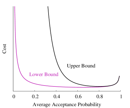
Figure 2: The cost of a Hamiltonian Monte Carlo implementation using the Metropolis proposal $\Phi^{\widetilde{H}}_{\epsilon,\tau}$ and a second-order symplectic integrator is squeezed between two approximate bounds that, up to a common scale, are universal for any target distribution and provide a general criteria for the optimal average acceptance probability or, equivalently, the integrator step size. Maximizing the approximate lower bound yields $a=0.651$ and minimizing the approximate upper bound suggests $a=0.801$; given that the approximate bounds are relatively flat, however, any value in between yields near-optimal results.

4 Limitations of the Step Size Optimization Criterion

When applying this optimization criterion we have to be careful to account for both the fundamental limitations in its construction and the possibility that the underlying assumptions may fail.

For example, although the cost function is applicable to both a constant integration time and an integration time chosen uniformly over some static distribution it is not applicable to an integration time that varies with the initial position, as would be necessary for a dynamically optimized integration time (Betancourt, 2013). Technically this precludes implementations of Hamiltonian Monte Carlo like the No-U-Turn sampler (Hoffman and Gelman, 2014), although in practice it has performed well as the default tuning mechanism for Stan (Stan Development Team, 2014a).

Similarly, the optimization criterion is only as good as the approximate bounds from which is it constructed. One source of error in these bounds are the high-order contributions beyond the Gaussian integral, although empirically these appear to be small for simple models (Figure 3). Because more complex models typically require smaller step sizes to achieve the same average acceptance probability, the higher-order contributions should continue to be negligible.

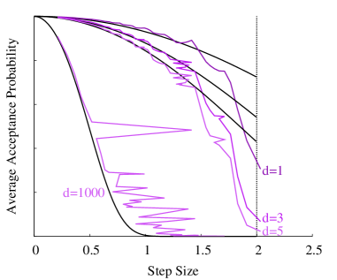
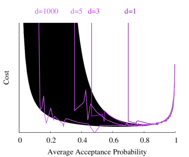
Figure 3: In experiments of Euclidean Hamiltonian Monte Carlo, implemented with a unit metric and second-order leapfrog integrator and targeting a product of independent Gaussian distributions, both (a) the relationship between integrator step size and average acceptance probability and (b) the relationship between the average acceptance probability and the cost are in excellent agreement with the approximations. In this case any higher-order corrections are negligible, at least until the step size approaches $\epsilon=2$ at which point the integrator becomes topologically unstable.

A more serious concern with the approximations is not in the neglected higher-order contributions but rather the assumption of topological stability and vanishing asymptotic error. In complex models the step sizes necessary for these conditions to hold can be much smaller than the step size motivated by the optimization strategy. Fortunately, when these conditions do not hold the integrator becomes unstable, manifesting almost immediately in numerical divergences that pull the state towards infinity and are readily incorporated into user-facing diagnostics. Consequently our initial optimization strategy can be made robust by monitoring these diagnostics and increasing the target average acceptance probability until no divergences occur (Figure 4). This more robust strategy has proven especially effective for hierarchical models that are particularly sensitive to this pathology (Betancourt and Girolami, 2015).

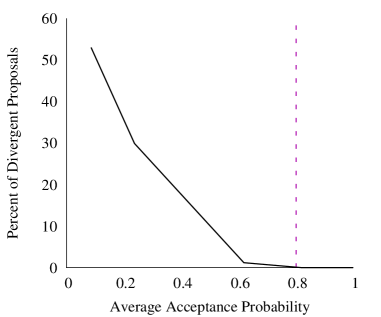
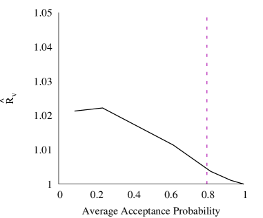
Figure 4: In complex problems careful monitoring of the step size optimization is critical towards ensuring a robust result. For example, in the (50 + 1)-dimensional funnel distribution Neal (2003) (a) numerical divergences begin to appear within the window of nominally-optimal acceptance probabilities which manifest as (c) an increasing potential scale reduction factor (Gelman and Rubin, 1992; Stan Development Team, 2014b), $\hat{R}_{v}$, that incorporates exact samples from the posterior. As the model complexity increases these inconsistencies become more severe and can result in biased Markov chains unless the optimization criterion is relaxed.

5 Conclusions and Future Work

By appealing to the underlying geometry of Hamiltonian Monte Carlo we have constructed a robust, universal scheme for the optimal tuning of the integrator step size, for for simple implementations of Hamiltonian Monte Carlo that use an approximate Hamiltonian flow to construct only a single Metropolis proposal.

The constructing of formal optimization criteria for more elaborate implementations of the algorithm, including windowed samplers (Neal, 1994), such as the No-U-Turn Sampler (Hoffman and Gelman, 2014), that subsample from each approximate trajectory, can also be placed into this geometric framework and utilize the theorems proved in this paper. Similarly, the understanding of canonical expectations we have built in this paper is applicable to Rao-Blackwellization schemes that keep all points along each approximate trajectory, using weights to correct for the error in the symplectic integrator.

6 Acknowledgements

We warmly thank Chris Wendl for illuminating discussions on various aspects of symplectic geometry used in the proofs and Elena Akhmatskaya for helpful comments. Michael Betancourt is supported under EPSRC grant EP/J016934/1, Simon Byrne is a EPSRC Postdoctoral Research Fellow under grant EP/K005723/1, and Mark Girolami is an EPSRC Established Career Research Fellow under grant EP/J016934/1.

A Proofs

Here we present proofs for the Lemmas and Theorems appearing in Sections 2.2 and 2.3, as well as a rigorous calculation of the average Hamiltonian error for the example in Section 2.3.

A.1 The Accuracy of Canonical Expectations

Theorem 1.

Let $\left(M,\omega,H\right)$ be a Hamiltonian system and consider a $k$-th order symmetric symplectic integrator with the corresponding modified Hamiltonian $\widetilde{H}=H+\epsilon^{k}\,G+\mathcal{O}(\epsilon^{k+2})$. If the integrator is topologically stable and the asymptotic error is negligible, then the difference in the microcanonical and modified microcanonical expectations for any smooth function, $f:M\rightarrow\mathbb{R}$, is given by

$$\left<f\right>_{H^{-1}\left(E\right)}-\left<f\right>_{\widetilde{H}^{-1}\left(E\right)}= +\epsilon^{k}\left<f\,\mathrm{d}G\!\left(\vec{v}\right)+G\,\mathrm{d}f\!\left(\vec{v}\right)+f\,G\left(\frac{\partial v^{i}}{\partial q^{i}}+\frac{\partial v_{i}}{\partial p_{i}}\right)\right>_{\widetilde{H}^{-1}\left(E\right)}$$

$$-\epsilon^{k}\Big{<}f\Big{>}_{\widetilde{H}^{-1}\left(E\right)}\left<\mathrm{d}G\!\left(\vec{v}\right)+G\left(\frac{\partial v^{i}}{\partial q^{i}}+\frac{\partial v_{i}}{\partial p_{i}}\right)\right>_{\widetilde{H}^{-1}\left(E\right)}+\mathcal{O}(\epsilon^{k+2}),$$

where $\vec{v}$ is any transverse vector field satisfying $\mathrm{d}H\!\left(\vec{v}\right)=1$.

Figure 5: Geometrically, a level set $H^{-1}\!\left(E\right)$ can be warped into a level set $\widetilde{H}^{-1}\!\left(E\right)$ by dragging it along the flow generated by $G\,\vec{v}$, admitting a comparison of expectations along the two surfaces.

Proof.

Provided that the integrator is stable and at the topologies of the level sets are the same, we can compare the two expectations by perturbing the true level set into the modified one by dragging it along $G\,\vec{v}$ (Figure 5). In particular, dragging the integrand gives

$$\left(f\,\vec{v}\,\lrcorner\,\Omega\right)^{\prime} =\int_{0}^{\epsilon^{k}}\mathrm{d}t\,\mathcal{L}_{G\,\vec{v}}\left(f\,\vec{v}\,\lrcorner\,\Omega\right)$$

$$=f\,\vec{v}\,\lrcorner\,\Omega+\epsilon^{k}\,\mathcal{L}_{G\,\vec{v}}\left(f\,\vec{v}\,\lrcorner\,\Omega\right)+\mathcal{O}(\epsilon^{k+2}).$$

The Lie derivative evaluates to

$$\mathcal{L}_{G\,\vec{v}}\left(f\,\vec{v}\,\lrcorner\,\Omega\right) =\mathcal{L}_{G\,\vec{v}}\left(f\right)\vec{v}\,\lrcorner\,\Omega+f\mathcal{L}_{G\,\vec{v}}\left(\vec{v}\,\lrcorner\,\Omega\right)$$

$$=\mathcal{L}_{G\,\vec{v}}\left(f\right)\vec{v}\,\lrcorner\,\Omega+f\big{[}G\,\vec{v},\vec{v}\big{]}\,\lrcorner\,\Omega+f\,\vec{v}\,\lrcorner\,\mathcal{L}_{G\,\vec{v}}\,\Omega,$$

where

$$\mathcal{L}_{G\,\vec{v}}\left(f\right) =G\,\mathrm{d}f\!\left(\vec{v}\right),$$

$$\big{[}G\,\vec{v},\vec{v}\big{]} =G\big{[}\vec{v},\vec{v}\big{]}-\mathrm{d}G\!\left(\vec{v}\right)\vec{v}$$

$$=-\mathrm{d}G\!\left(\vec{v}\right)\vec{v},$$

and

$$\mathcal{L}_{G\,\vec{v}}\,\Omega =G\,\mathcal{L}_{\vec{v}}\,\Omega+\mathrm{d}G\wedge\left(\vec{v}\,\lrcorner\,\Omega\right)$$

$$=G\,\vec{v}\,\lrcorner\,\mathrm{d}\Omega+G\,\mathrm{d}\!\left(\vec{v}\,\lrcorner\,\Omega\right)+\mathrm{d}G\wedge\left(\vec{v}\,\lrcorner\,\Omega\right)$$

$$=G\,\mathrm{d}\!\left(\vec{v}\,\lrcorner\,\Omega\right)+\mathrm{d}G\wedge\left(\vec{v}\,\lrcorner\,\Omega\right)$$

$$=G\,\mathrm{d}\!\left(\vec{v}\,\lrcorner\,\Omega\right)+\mathrm{d}G\!\left(\vec{v}\right)\,\lrcorner\,\Omega-\vec{v}\,\lrcorner\,\left(\mathrm{d}G\wedge\Omega\right)$$

$$=G\,\mathrm{d}\!\left(\vec{v}\,\lrcorner\,\Omega\right)+\mathrm{d}G\!\left(\vec{v}\right)\,\lrcorner\,\Omega.$$

Hence

$$\mathcal{L}_{G\,\vec{v}}\left(f\vec{v}\,\lrcorner\,\Omega\right) =G\,\mathrm{d}f\!\left(\vec{v}\right)\vec{v}\,\lrcorner\,\Omega-f\,\mathrm{d}G\!\left(\vec{v}\right)\vec{v}\,\lrcorner\,\Omega+f\,G\,\vec{v}\,\lrcorner\,\mathrm{d}\left(\vec{v}\,\lrcorner\,\Omega\right)+f\,\mathrm{d}G\!\left(\vec{v}\right)\vec{v}\,\lrcorner\,\Omega$$

$$=G\,\mathrm{d}f\!\left(\vec{v}\right)\vec{v}\,\lrcorner\,\Omega+f\,G\,\vec{v}\,\lrcorner\,\mathrm{d}\left(\vec{v}\,\lrcorner\,\Omega\right),$$

or, in canonical coordinates,

$$\mathcal{L}_{G\,\vec{v}}\left(f\vec{v}\,\lrcorner\,\Omega\right)=G\,\mathrm{d}f\!\left(\vec{v}\right)\vec{v}\,\lrcorner\,\Omega+f\,G\left(\frac{\partial v^{i}}{\partial q^{i}}+\frac{\partial v_{i}}{\partial p_{i}}\right)\vec{v}\,\lrcorner\,\Omega.$$

Together these give

$$\left(f\,\vec{v}\,\lrcorner\,\Omega\right)^{\prime}=\left(f+\epsilon^{k}\,G\,\mathrm{d}f\!\left(\vec{v}\right)+\epsilon^{k}\,f\,G\left(\frac{\partial v^{i}}{\partial q^{i}}+\frac{\partial v_{i}}{\partial p_{i}}\right)\right)\vec{v}\,\lrcorner\,\Omega+\mathcal{O}(\epsilon^{k+2}),$$

Before we can pull these terms onto $\widetilde{H}^{-1}\!\left(E\right)$ we have to relate them to the proper volume form, $\vec{u}\,\lrcorner\,\Omega$. Because

$$\vec{v}\,\lrcorner\,\Omega =\mathrm{d}\widetilde{H}\!\left(\vec{v}\right)\vec{u}\,\lrcorner\,\Omega$$

$$=\left(\mathrm{d}H\!\left(\vec{v}\right)+\epsilon^{k}\,\mathrm{d}G\!\left(\vec{v}\right)\right)\vec{u}\,\lrcorner\,\Omega$$

$$=\left(1+\epsilon^{k}\,\mathrm{d}G\!\left(\vec{v}\right)\right)\vec{u}\,\lrcorner\,\Omega,$$

we have, to leading-order in the step size,

$$\left(f\,\vec{v}\,\lrcorner\,\Omega\right)^{\prime}=f\vec{u}\,\lrcorner\,\Omega+\epsilon^{k}\left(f\,\mathrm{d}G\!\left(\vec{v}\right)+G\,\mathrm{d}f\!\left(\vec{v}\right)+f\,G\left(\frac{\partial v^{i}}{\partial q^{i}}+\frac{\partial v_{i}}{\partial p_{i}}\right)\right)\vec{u}\,\lrcorner\,\Omega+\mathcal{O}(\epsilon^{k+2}),$$

Pulling back onto the modified level set gives

$$\int_{H^{-1}\left(E\right)}\iota^{*}_{E}\left(f\,\vec{v}\,\lrcorner\,\Omega\right)= \int_{\widetilde{H}^{-1}\left(E\right)}\tilde{\iota}^{*}_{E}\left(f\,\vec{v}\,\lrcorner\,\Omega\right)^{\prime}$$

$$= \int_{\widetilde{H}^{-1}\left(E\right)}\tilde{\iota}^{*}_{E}\!\left(f\,\vec{u}\,\lrcorner\,\Omega\right)$$

$$+\epsilon^{k}\int_{\widetilde{H}^{-1}\left(E\right)}\tilde{\iota}^{*}_{E}\!\left(\left(f\,\mathrm{d}G\!\left(\vec{v}\right)+G\,\mathrm{d}f\!\left(\vec{v}\right)+f\,G\left(\frac{\partial v^{i}}{\partial q^{i}}+\frac{\partial v_{i}}{\partial p_{i}}\right)\right)\vec{u}\,\lrcorner\,\Omega\right)+\mathcal{O}(\epsilon^{k+2}),$$

Consequently the microcanonical expectation becomes

$$\left<f\right>_{H^{-1}\left(E\right)}= \frac{\int_{H^{-1}\left(E\right)}\iota^{*}_{E}\!\left(f\,\vec{v}\,\lrcorner\,\Omega\right)}{\int_{H^{-1}\left(E\right)}\iota^{*}_{E}\!\left(\vec{v}\,\lrcorner\,\Omega\right)}$$

$$= \frac{\int_{\widetilde{H}^{-1}\left(E\right)}\tilde{\iota}^{*}_{E}\!\left(f\,\vec{u}\,\lrcorner\,\Omega\right)+\epsilon^{k}\int_{\widetilde{H}^{-1}\left(E\right)}\tilde{\iota}^{*}_{E}\!\left(\left(f\,\mathrm{d}G\!\left(\vec{v}\right)+G\,\mathrm{d}f\!\left(\vec{v}\right)+f\,G\left(\frac{\partial v^{i}}{\partial q^{i}}+\frac{\partial v_{i}}{\partial p_{i}}\right)\right)\vec{u}\,\lrcorner\,\Omega\right)}{\int_{\widetilde{H}^{-1}\left(E\right)}\tilde{\iota}^{*}_{E}\!\left(\vec{u}\,\lrcorner\,\Omega\right)+\epsilon^{k}\int_{\widetilde{H}^{-1}\left(E\right)}\tilde{\iota}^{*}_{E}\!\left(\left(\mathrm{d}G\!\left(\vec{v}\right)+G\left(\frac{\partial v^{i}}{\partial q^{i}}+\frac{\partial v_{i}}{\partial p_{i}}\right)\right)\vec{u}\,\lrcorner\,\Omega\right)}$$

$$+\mathcal{O}(\epsilon^{2k})$$

$$= \frac{\int_{\widetilde{H}^{-1}\left(E\right)}\tilde{\iota}^{*}_{E}\!\left(f\,\vec{u}\,\lrcorner\,\Omega\right)}{\int_{\widetilde{H}^{-1}\left(E\right)}\tilde{\iota}^{*}_{E}\!\left(\vec{u}\,\lrcorner\,\Omega\right)}$$

$$+\epsilon^{k}\frac{\int_{\widetilde{H}^{-1}\left(E\right)}\tilde{\iota}^{*}_{E}\!\left(\left(f\,\mathrm{d}G\!\left(\vec{v}\right)+G\,\mathrm{d}f\!\left(\vec{v}\right)+f\,G\left(\frac{\partial v^{i}}{\partial q^{i}}+\frac{\partial v_{i}}{\partial p_{i}}\right)\right)\vec{u}\,\lrcorner\,\Omega\right)}{\int_{\widetilde{H}^{-1}\left(E\right)}\tilde{\iota}^{*}_{E}\!\left(\vec{u}\,\lrcorner\,\Omega\right)}$$

$$-\epsilon^{k}\frac{\int_{\widetilde{H}^{-1}\left(E\right)}\tilde{\iota}^{*}_{E}\!\left(f\,\vec{u}\,\lrcorner\,\Omega\right)}{\int_{\widetilde{H}^{-1}\left(E\right)}\tilde{\iota}^{*}_{E}\!\left(\vec{u}\,\lrcorner\,\Omega\right)}\frac{\int_{\widetilde{H}^{-1}\left(E\right)}\tilde{\iota}^{*}_{E}\!\left(\left(\mathrm{d}G\!\left(\vec{v}\right)+G\left(\frac{\partial v^{i}}{\partial q^{i}}+\frac{\partial v_{i}}{\partial p_{i}}\right)\right)\vec{u}\,\lrcorner\,\Omega\right)}{\int_{\widetilde{H}^{-1}\left(E\right)}\tilde{\iota}^{*}_{E}\!\left(\vec{u}\,\lrcorner\,\Omega\right)}+\mathcal{O}(\epsilon^{k+2})$$

$$= \left<f\right>_{\widetilde{H}^{-1}\left(E\right)}+\epsilon^{k}\left<f\,\mathrm{d}G\!\left(\vec{v}\right)+G\,\mathrm{d}f\!\left(\vec{v}\right)+f\,G\left(\frac{\partial v^{i}}{\partial q^{i}}+\frac{\partial v_{i}}{\partial p_{i}}\right)\right>_{\widetilde{H}^{-1}\left(E\right)}$$

$$-\epsilon^{k}\left<f\right>_{\widetilde{H}^{-1}\left(E\right)}\left<\mathrm{d}G\!\left(\vec{v}\right)+G\left(\frac{\partial v^{i}}{\partial q^{i}}+\frac{\partial v_{i}}{\partial p_{i}}\right)\right>_{\widetilde{H}^{-1}\left(E\right)}+\mathcal{O}(\epsilon^{k+2}),$$

or

$$\left<f\right>_{H^{-1}\left(E\right)}-\left<f\right>_{\widetilde{H}^{-1}\left(E\right)}= +\epsilon^{k}\left<f\,\mathrm{d}G\!\left(\vec{v}\right)+G\,\mathrm{d}f\!\left(\vec{v}\right)+f\,G\left(\frac{\partial v^{i}}{\partial q^{i}}+\frac{\partial v_{i}}{\partial p_{i}}\right)\right>_{\widetilde{H}^{-1}\left(E\right)}$$

$$-\epsilon^{k}\left<f\right>_{\widetilde{H}^{-1}\left(E\right)}\left<\mathrm{d}G\!\left(\vec{v}\right)+G\left(\frac{\partial v^{i}}{\partial q^{i}}+\frac{\partial v_{i}}{\partial p_{i}}\right)\right>_{\widetilde{H}^{-1}\left(E\right)}+\mathcal{O}(\epsilon^{k+2}),$$

as desired.

∎

Corollary 10.

Let $\left(M,\omega,H\right)$ be a Hamiltonian system and consider a $k$-th order symmetric symplectic integrator with the corresponding modified Hamiltonian $\widetilde{H}=H+\epsilon^{k}\,G+\mathcal{O}(\epsilon^{k+2})$. If the integrator is topologically stable and the asymptotic error is negligible then

$$\frac{1}{\int_{M}e^{-\beta H}\Omega} =\frac{1}{\int_{M}e^{-\beta\widetilde{H}}\Omega}\left(1-\epsilon^{k}\,\mathbb{E}_{\varpi_{\widetilde{H}}}\!\left[\mathrm{d}G\!\left(\vec{v}\right)+G\left(\frac{\partial v^{i}}{\partial q^{i}}+\frac{\partial v_{i}}{\partial p_{i}}\right)\right]\right)+\mathcal{O}(\epsilon^{k+2})$$

where $\vec{v}$ is any transverse vector field satisfying $\mathrm{d}H\!\left(\vec{v}\right)=1$.

Proof.

Taking $f=1$ in the derivation Theorem 1 we have

$$d\!\left(E\right) =\int_{H^{-1}\left(E\right)}\iota^{*}_{E}\!\left(\vec{v}\,\lrcorner\,\Omega\right)$$

$$=\int_{\widetilde{H}^{-1}\left(E\right)}\tilde{\iota}^{*}_{E}\!\left(\vec{u}\,\lrcorner\,\Omega\right)$$

$$\quad+\epsilon^{k}\int_{\widetilde{H}^{-1}\left(E\right)}\tilde{\iota}^{*}_{E}\!\left(\left(\mathrm{d}G\!\left(\vec{v}\right)+G\left(\frac{\partial v^{i}}{\partial q^{i}}+\frac{\partial v_{i}}{\partial p_{i}}\right)\right)\vec{u}\,\lrcorner\,\Omega\right)+\mathcal{O}(\epsilon^{k+2})$$

$$\equiv\tilde{d}\!\left(E\right)+\epsilon^{k}\,d^{\prime}\!\left(E\right)+\mathcal{O}(\epsilon^{k+2}).$$

Then

$$\frac{1}{\int_{M}e^{-\beta H}\Omega} =\frac{1}{\int\mathrm{d}E\,d\!\left(E\right)e^{-\beta E}}$$

$$=\frac{1}{\int\mathrm{d}E\,\left(\tilde{d}\!\left(E\right)+\epsilon^{k}\,d^{\prime}\!\left(E\right)+\mathcal{O}(\epsilon^{k+2})\right)e^{-\beta E}}$$

$$=\frac{1}{\int\mathrm{d}E\,\tilde{d}\!\left(E\right)e^{-\beta E}+\epsilon^{k}\,\int\mathrm{d}E\,e^{-\beta E}d^{\prime}\!\left(E\right)+\mathcal{O}(\epsilon^{k+2})}$$

$$=\frac{1}{\int\mathrm{d}E\,\tilde{d}\!\left(E\right)e^{-\beta E}}\left(1-\epsilon^{k}\,\frac{\int\mathrm{d}E\,e^{-\beta E}d^{\prime}\!\left(E\right)}{\int\mathrm{d}E\,\tilde{d}\!\left(E\right)e^{-\beta E}}\right)+\mathcal{O}(\epsilon^{k+2})$$

$$=\frac{1}{\int\mathrm{d}E\,\tilde{d}\!\left(E\right)e^{-\beta E}}\left(1-\epsilon^{k}\,\mathbb{E}_{\varpi_{\widetilde{H}}}\!\left[d^{\prime}\!\left(E\right)\right]\right)+\mathcal{O}(\epsilon^{k+2})$$

$$=\frac{1}{\int_{M}e^{-\beta\widetilde{H}}\Omega}\left(1-\epsilon^{k}\,\mathbb{E}_{\varpi_{\widetilde{H}}}\!\left[d^{\prime}\!\left(E\right)\right]\right)+\mathcal{O}(\epsilon^{k+2})$$

or

$$\frac{1}{\int_{M}e^{-\beta H}\Omega} =\frac{1}{\int_{M}e^{-\beta\widetilde{H}}\Omega}\left(1-\epsilon^{k}\,\mathbb{E}_{\varpi_{\widetilde{H}}}\!\left[\mathrm{d}G\!\left(\vec{v}\right)+G\left(\frac{\partial v^{i}}{\partial q^{i}}+\frac{\partial v_{i}}{\partial p_{i}}\right)\right]\right)+\mathcal{O}(\epsilon^{k+2}),$$

as desired.

∎

Theorem 2.

Let $\left(M,\omega,H\right)$ be a Hamiltonian system and consider a $k$-th order symmetric symplectic integrator with the corresponding modified Hamiltonian $\widetilde{H}=H+\epsilon^{k}\,G+\mathcal{O}(\epsilon^{k+2})$. If the integrator is topologically stable and the asymptotic error is negligible, then the difference in the canonical and modified canonical expectations for any smooth function, $f:M\rightarrow\mathbb{R}$, is given by

$$\mathbb{E}_{\varpi_{H}}\!\left[f\right]-\mathbb{E}_{\varpi_{\widetilde{H}}}\!\left[f\right]= +\epsilon^{k}\,\mathbb{E}_{\varpi_{H}}\!\left[f\,\mathrm{d}G\!\left(\vec{v}\right)+G\,\mathrm{d}f\!\left(\vec{v}\right)+f\,G\left(\frac{\partial v^{i}}{\partial q^{i}}+\frac{\partial v_{i}}{\partial p_{i}}\right)\right]$$

$$-\epsilon^{k}\,\mathbb{E}_{\varpi_{H}}\!\left[f\right]\,\mathbb{E}_{\varpi_{H}}\!\left[\mathrm{d}G\!\left(\vec{v}\right)+G\left(\frac{\partial v^{i}}{\partial q^{i}}+\frac{\partial v_{i}}{\partial p_{i}}\right)\right]+\mathcal{O}(\epsilon^{k+2}),$$

where $\vec{v}$ is any transverse vector field satisfying $\mathrm{d}H\!\left(\vec{v}\right)=1$.

Proof.

Applying Theorem 1,

$$\int_{H^{-1}\left(E\right)}\iota^{*}_{E}\left(f\,\vec{v}\,\lrcorner\,\Omega\right) =\int_{\widetilde{H}^{-1}\left(E\right)}\tilde{\iota}^{*}_{E}\!\left(f\,\vec{u}\,\lrcorner\,\Omega\right)$$

$$\quad+\epsilon^{k}\int_{\widetilde{H}^{-1}\left(E\right)}\tilde{\iota}^{*}_{E}\!\left(\left(f\,\mathrm{d}G\!\left(\vec{v}\right)+G\,\mathrm{d}f\!\left(\vec{v}\right)+f\,G\left(\frac{\partial v^{i}}{\partial q^{i}}+\frac{\partial v_{i}}{\partial p_{i}}\right)\right)\vec{u}\,\lrcorner\,\Omega\right)$$

$$\quad+\mathcal{O}(\epsilon^{k+2})$$

$$\equiv\mathcal{I}+\epsilon^{k}\,\mathcal{I}^{\prime}+\mathcal{O}(\epsilon^{k+2}),$$

and

$$d\!\left(E\right) =\int_{H^{-1}\left(E\right)}\iota^{*}_{E}\!\left(\vec{v}\,\lrcorner\,\Omega\right)$$

$$=\int_{\widetilde{H}^{-1}\left(E\right)}\tilde{\iota}^{*}_{E}\!\left(\vec{u}\,\lrcorner\,\Omega\right)$$

$$\quad+\epsilon^{k}\int_{\widetilde{H}^{-1}\left(E\right)}\tilde{\iota}^{*}_{E}\!\left(\left(\mathrm{d}G\!\left(\vec{v}\right)+G\left(\frac{\partial v^{i}}{\partial q^{i}}+\frac{\partial v_{i}}{\partial p_{i}}\right)\right)\vec{u}\,\lrcorner\,\Omega\right)+\mathcal{O}(\epsilon^{k+2})$$

$$\equiv\tilde{d}\!\left(E\right)+\epsilon^{k}\,d^{\prime}\!\left(E\right)+\mathcal{O}(\epsilon^{k+2}).$$

Substituting these into the definition of the canonical expectation gives

$$\mathbb{E}_{\varpi_{H}}\!\left[f\right] =\frac{\int\mathrm{d}E\,e^{-\beta E}\int_{H^{-1}\left(E\right)}\iota^{*}_{E}\!\left(f\,\vec{v}\,\lrcorner\,\Omega\right)}{\int\mathrm{d}E\,d\!\left(E\right)e^{-\beta E}}$$

$$=\frac{\int\mathrm{d}E\,e^{-\beta E}\left(\mathcal{I}+\epsilon^{k}\,\mathcal{I}^{\prime}+\mathcal{O}(\epsilon^{k+2})\right)}{\int\mathrm{d}E\,e^{-\beta E}\left(\tilde{d}\!\left(E\right)+\epsilon^{k}\,d^{\prime}\!\left(E\right)+\mathcal{O}(\epsilon^{k+2})\right)}$$

$$=\frac{\int\mathrm{d}E\,e^{-\beta E}\mathcal{I}}{\int\mathrm{d}E\,e^{-\beta E}\tilde{d}\!\left(E\right)}+\delta\frac{\int\mathrm{d}E\,e^{-\beta E}\mathcal{I}^{\prime}}{\int\mathrm{d}E\,e^{-\beta E}\tilde{d}\!\left(E\right)}-\delta\frac{\int\mathrm{d}E\,e^{-\beta E}\mathcal{I}}{\int\mathrm{d}E\,e^{-\beta E}\tilde{d}\!\left(E\right)}\frac{\int\mathrm{d}E\,e^{-\beta E}d^{\prime}\!\left(E\right)}{\int\mathrm{d}E\,e^{-\beta E}\tilde{d}\!\left(E\right)}+\mathcal{O}(\epsilon^{k+2})$$

$$=+\frac{\int\mathrm{d}E\,e^{-\beta E}\int_{\widetilde{H}^{-1}\left(E\right)}\tilde{\iota}^{*}_{E}\!\left(f\,\vec{u}\,\lrcorner\,\Omega\right)}{\int\mathrm{d}E\,\tilde{d}\!\left(E\right)e^{-\beta E}}$$

$$\quad+\epsilon^{k}\frac{\int\mathrm{d}E\,e^{-\beta E}\epsilon^{k}\int_{\widetilde{H}^{-1}\left(E\right)}\tilde{\iota}^{*}_{E}\!\left(\left(f\,\mathrm{d}G\!\left(\vec{v}\right)+G\,\mathrm{d}f\!\left(\vec{v}\right)+f\,G\left(\frac{\partial v^{i}}{\partial q^{i}}+\frac{\partial v_{i}}{\partial p_{i}}\right)\right)\vec{u}\,\lrcorner\,\Omega\right)}{\int\mathrm{d}E\,\tilde{d}\!\left(E\right)e^{-\beta E}}$$

$$\quad-\epsilon^{k}\frac{\int\mathrm{d}E\,e^{-\beta E}\int_{\widetilde{H}^{-1}\left(E\right)}\tilde{\iota}^{*}_{E}\!\left(f\,\vec{u}\,\lrcorner\,\Omega\right)}{\int\mathrm{d}E\,\tilde{d}\!\left(E\right)e^{-\beta E}}\frac{\int\mathrm{d}E\,e^{-\beta E}\int_{\widetilde{H}^{-1}\left(E\right)}\tilde{\iota}^{*}_{E}\!\left(\left(\mathrm{d}G\!\left(\vec{v}\right)+G\left(\frac{\partial v^{i}}{\partial q^{i}}+\frac{\partial v_{i}}{\partial p_{i}}\right)\right)\vec{u}\,\lrcorner\,\Omega\right)}{\int\mathrm{d}E\,\tilde{d}\!\left(E\right)e^{-\beta E}}$$

$$\quad+\mathcal{O}(\epsilon^{k+2})$$

$$=+\mathbb{E}_{\varpi_{\widetilde{H}}}\!\Big{[}f\Big{]}+\epsilon^{k}\,\mathbb{E}_{\varpi_{\widetilde{H}}}\!\left[f\,\mathrm{d}G\!\left(\vec{v}\right)+G\,\mathrm{d}f\!\left(\vec{v}\right)+f\,G\left(\frac{\partial v^{i}}{\partial q^{i}}+\frac{\partial v_{i}}{\partial p_{i}}\right)\right]$$

$$\quad-\epsilon^{k}\,\mathbb{E}_{\varpi_{\widetilde{H}}}\!\Big{[}f\Big{]}\mathbb{E}_{\varpi_{\widetilde{H}}}\!\left[\mathrm{d}G\!\left(\vec{v}\right)+G\left(\frac{\partial v^{i}}{\partial q^{i}}+\frac{\partial v_{i}}{\partial p_{i}}\right)\right]+\mathcal{O}(\epsilon^{k+2}),$$

or

$$\mathbb{E}_{\varpi_{H}}\!\left[f\right]-\mathbb{E}_{\varpi_{\widetilde{H}}}\!\left[f\right] =+\epsilon^{k}\,\mathbb{E}_{\varpi_{\widetilde{H}}}\!\left[f\,\mathrm{d}G\!\left(\vec{v}\right)+G\,\mathrm{d}f\!\left(\vec{v}\right)+f\,G\left(\frac{\partial v^{i}}{\partial q^{i}}+\frac{\partial v_{i}}{\partial p_{i}}\right)\right]$$

$$\quad-\epsilon^{k}\,\mathbb{E}_{\varpi_{\widetilde{H}}}\!\Big{[}f\Big{]}\mathbb{E}_{\varpi_{\widetilde{H}}}\!\left[\mathrm{d}G\!\left(\vec{v}\right)+G\left(\frac{\partial v^{i}}{\partial q^{i}}+\frac{\partial v_{i}}{\partial p_{i}}\right)\right]+\mathcal{O}(\epsilon^{k+2}),$$

as desired.

∎

A.2 Approximating Canonical Expectations of the Hamiltonian Error

In order to compute moments of the Hamiltonian error we first have to be able to manipulate the Metropolis proposal operator, $\Phi^{\widetilde{H}}_{\epsilon,\tau}$. Fortunately, the operator is a diffeomorphism, $\Phi^{\widetilde{H}}_{\epsilon,\tau}:M\rightarrow M$ which admits a variety of convenient manipulations.

Lemma 11.

“Correlation by Parts”. Let $\left(M,\omega,H\right)$ be a Hamiltonian system and consider a $k$-th order symmetric symplectic integrator with the corresponding modified Hamiltonian $\widetilde{H}=H+\epsilon^{k}\,G+\mathcal{O}(\epsilon^{k+2})$ and Metropolis proposal $\Phi^{\widetilde{H}}_{\epsilon,\tau}$. If the integrator is topologically stable and the asymptotic error is negligible, then the correlation of two smooth functions, $f:M\rightarrow\mathbb{R}$ and $h:M\rightarrow\mathbb{R}$, with respect to a unit canonical distribution satisfies

$$\mathbb{E}_{\varpi_{H}}\!\left[f\left(h\circ\Phi^{\widetilde{H}}_{\epsilon,\tau}\right)\right] =\mathbb{E}_{\varpi_{\widetilde{H}}}\!\left[\left(f\circ\Phi^{\widetilde{H}}_{\epsilon,\tau}\right)h\right]$$

$$\quad+\epsilon^{k}\Big{(}-\mathbb{E}_{\varpi_{H}}\!\left[f\left(h\circ\Phi^{\widetilde{H}}_{\epsilon,\tau}\right)\right]\mathbb{E}_{\varpi_{\widetilde{H}}}\!\left[\mathrm{d}G\!\left(\vec{v}\right)+G\left(\frac{\partial v^{i}}{\partial q^{i}}+\frac{\partial v_{i}}{\partial p_{i}}\right)\right]$$

$$\quad\quad\quad\;+\mathbb{E}_{\varpi_{\widetilde{H}}}\!\left[\left(f\circ\Phi^{\widetilde{H}}_{\epsilon,\tau}\right)h\,\left(G\circ\Phi^{\widetilde{H}}_{\epsilon,\tau}\right)\right]\Big{)}$$

$$\quad+\mathcal{O}(\epsilon^{k+2}),$$

where $\vec{v}$ is any transverse vector field satisfying $\mathrm{d}H\!\left(\vec{v}\right)=1$.

Proof.

By definition

$$\mathbb{E}_{\varpi_{H}}\!\left[f\left(h\circ\Phi^{\widetilde{H}}_{\epsilon,\tau}\right)\right]=\frac{\int_{M}f\left(h\circ\Phi^{\widetilde{H}}_{\epsilon,\tau}\right)e^{-H}\Omega}{\int_{M}e^{-H}\Omega}$$

Because $\Phi^{\widetilde{H}}_{\epsilon,\tau}$ is a diffeomorphism we can push-forward integrals; in particular the numerator becomes

$$\int_{M}f\left(h\circ\Phi^{\widetilde{H}}_{\epsilon,\tau}\right)e^{-H}\Omega =\int_{M}\left(\Phi^{\widetilde{H}}_{\epsilon,\tau}\right)^{*}\left(f\left(h\circ\Phi^{\widetilde{H}}_{\epsilon,\tau}\right)e^{-H}\Omega\right)$$

$$=\int_{M}\left(f\circ\Phi^{\widetilde{H}}_{\epsilon,\tau}\right)\left(h\circ\Phi^{\widetilde{H}}_{\epsilon,\tau}\circ\Phi^{\widetilde{H}}_{\epsilon,\tau}\right)e^{-H\circ\Phi^{\widetilde{H}}_{\epsilon,\tau}}\Omega$$

$$=\int_{M}\left(f\circ\Phi^{\widetilde{H}}_{\epsilon,\tau}\right)h\,e^{-H\circ\Phi^{\widetilde{H}}_{\epsilon,\tau}}\Omega,$$

where we have used the fact that $\Phi^{\widetilde{H}}_{\epsilon,\tau}$ is idempotent. Substituting the definition of the modified Hamiltonian into the exponent and expanding then gives

$$\int_{M}f\left(h\circ\Phi^{\widetilde{H}}_{\epsilon,\tau}\right)e^{-H}\Omega =\int_{M}\left(f\circ\Phi^{\widetilde{H}}_{\epsilon,\tau}\right)h\,e^{-H\circ\Phi^{\widetilde{H}}_{\epsilon,\tau}}\Omega$$

$$=\int_{M}\left(f\circ\Phi^{\widetilde{H}}_{\epsilon,\tau}\right)h\,e^{-\left(\widetilde{H}-\epsilon^{k}\,G\right)\circ\Phi^{\widetilde{H}}_{\epsilon,\tau}}\Omega$$

$$=\int_{M}\left(f\circ\Phi^{\widetilde{H}}_{\epsilon,\tau}\right)h\,e^{-\widetilde{H}\circ\Phi^{\widetilde{H}}_{\epsilon,\tau}}e^{\epsilon^{k}\,G\circ\Phi^{\widetilde{H}}_{\epsilon,\tau}}\Omega$$

$$=\int_{M}\left(f\circ\Phi^{\widetilde{H}}_{\epsilon,\tau}\right)h\,e^{-\widetilde{H}\circ\Phi^{\widetilde{H}}_{\epsilon,\tau}}\left(1+\epsilon^{k}\,G\circ\Phi^{\widetilde{H}}_{\epsilon,\tau}\right)\Omega+\mathcal{O}(\epsilon^{k+2})$$

$$=\int_{M}\left(f\circ\Phi^{\widetilde{H}}_{\epsilon,\tau}\right)h\,e^{-\widetilde{H}\circ\Phi^{\widetilde{H}}_{\epsilon,\tau}}\Omega$$

$$\quad+\epsilon^{k}\int_{M}\left(f\circ\Phi^{\widetilde{H}}_{\epsilon,\tau}\right)h\,\left(G\circ\Phi^{\widetilde{H}}_{\epsilon,\tau}\right)e^{-\widetilde{H}\circ\Phi^{\widetilde{H}}_{\epsilon,\tau}}\Omega+\mathcal{O}(\epsilon^{k+2}).$$

But the modified Hamiltonian is invariant to the modified flow, $\widetilde{H}\circ\Phi^{\widetilde{H}}_{\epsilon,\tau}=\widetilde{H}$ and the integrals on the RHS become

$$\int_{M}f\left(h\circ\Phi^{\widetilde{H}}_{\epsilon,\tau}\right)e^{-H}\Omega =\int_{M}\left(f\circ\Phi^{\widetilde{H}}_{\epsilon,\tau}\right)h\,e^{-\widetilde{H}}\Omega$$

$$\quad+\epsilon^{k}\int_{M}\left(f\circ\Phi^{\widetilde{H}}_{\epsilon,\tau}\right)h\,\left(G\circ\Phi^{\widetilde{H}}_{\epsilon,\tau}\right)e^{-\widetilde{H}}\Omega+\mathcal{O}(\epsilon^{k+2}).$$

Dividing by the modified normalization,

$$\frac{\int_{M}f\left(h\circ\Phi^{\widetilde{H}}_{\epsilon,\tau}\right)e^{-H}\Omega}{\int_{M}e^{-\widetilde{H}}\Omega} =\frac{\int_{M}\left(f\circ\Phi^{\widetilde{H}}_{\epsilon,\tau}\right)h\,e^{-\widetilde{H}}\Omega}{\int_{M}e^{-\widetilde{H}}\Omega}+\epsilon^{k}\frac{\int_{M}\left(f\circ\Phi^{\widetilde{H}}_{\epsilon,\tau}\right)h\,\left(G\circ\Phi^{\widetilde{H}}_{\epsilon,\tau}\right)e^{-\widetilde{H}}\Omega}{\int_{M}e^{-\widetilde{H}}\Omega}+\mathcal{O}(\epsilon^{k+2})$$

$$=\mathbb{E}_{\varpi_{\widetilde{H}}}\!\left[\left(f\circ\Phi^{\widetilde{H}}_{\epsilon,\tau}\right)h\right]+\epsilon^{k}\,\mathbb{E}_{\varpi_{\widetilde{H}}}\!\left[\left(f\circ\Phi^{\widetilde{H}}_{\epsilon,\tau}\right)h\,\left(G\circ\Phi^{\widetilde{H}}_{\epsilon,\tau}\right)\right]+\mathcal{O}(\epsilon^{k+2}).$$

Finally, we apply Corollary 10 to replace the modified normalization on the LHS with the true normalization and the necessary correction,

$$\frac{\int_{M}f\left(h\circ\Phi^{\widetilde{H}}_{\epsilon,\tau}\right)e^{-H}\Omega}{\int_{M}e^{-H}\Omega}\left(1+\epsilon^{k}\,\mathbb{E}_{\varpi_{\widetilde{H}}}\!\left[\mathrm{d}G\!\left(\vec{v}\right)+G\left(\frac{\partial v^{i}}{\partial q^{i}}+\frac{\partial v_{i}}{\partial p_{i}}\right)\right]\right) =$$

$$\mathbb{E}_{\varpi_{\widetilde{H}}}\!\left[\left(f\circ\Phi^{\widetilde{H}}_{\epsilon,\tau}\right)h\right]+\epsilon^{k}\,\mathbb{E}_{\varpi_{\widetilde{H}}}\!\left[\left(f\circ\Phi^{\widetilde{H}}_{\epsilon,\tau}\right)h\,\left(G\circ\Phi^{\widetilde{H}}_{\epsilon,\tau}\right)\right]+\mathcal{O}(\epsilon^{k+2})$$

$$\mathbb{E}_{\varpi_{H}}\!\left[f\left(h\circ\Phi^{\widetilde{H}}_{\epsilon,\tau}\right)\right]+\epsilon^{k}\,\mathbb{E}_{\varpi_{H}}\!\left[f\left(h\circ\Phi^{\widetilde{H}}_{\epsilon,\tau}\right)\right]\mathbb{E}_{\varpi_{\widetilde{H}}}\!\left[\mathrm{d}G\!\left(\vec{v}\right)+G\left(\frac{\partial v^{i}}{\partial q^{i}}+\frac{\partial v_{i}}{\partial p_{i}}\right)\right] =$$

$$\mathbb{E}_{\varpi_{\widetilde{H}}}\!\left[\left(f\circ\Phi^{\widetilde{H}}_{\epsilon,\tau}\right)h\right]+\epsilon^{k}\,\mathbb{E}_{\varpi_{\widetilde{H}}}\!\left[\left(f\circ\Phi^{\widetilde{H}}_{\epsilon,\tau}\right)h\,\left(G\circ\Phi^{\widetilde{H}}_{\epsilon,\tau}\right)\right]+\mathcal{O}(\epsilon^{k+2}),$$

or

$$\mathbb{E}_{\varpi_{H}}\!\left[f\left(h\circ\Phi^{\widetilde{H}}_{\epsilon,\tau}\right)\right] =\mathbb{E}_{\varpi_{\widetilde{H}}}\!\left[\left(f\circ\Phi^{\widetilde{H}}_{\epsilon,\tau}\right)h\right]$$

$$\quad+\epsilon^{k}\Big{(}-\mathbb{E}_{\varpi_{H}}\!\left[f\left(h\circ\Phi^{\widetilde{H}}_{\epsilon,\tau}\right)\right]\mathbb{E}_{\varpi_{\widetilde{H}}}\!\left[\mathrm{d}G\!\left(\vec{v}\right)+G\left(\frac{\partial v^{i}}{\partial q^{i}}+\frac{\partial v_{i}}{\partial p_{i}}\right)\right]$$

$$\quad\quad\quad\;+\mathbb{E}_{\varpi_{\widetilde{H}}}\!\left[\left(f\circ\Phi^{\widetilde{H}}_{\epsilon,\tau}\right)h\,\left(G\circ\Phi^{\widetilde{H}}_{\epsilon,\tau}\right)\right]\Big{)}$$

$$\quad+\mathcal{O}(\epsilon^{k+2}),$$

as desired.

∎

Now can compute the scaling of the moments of the Hamiltonian error, $\Delta_{\epsilon}$.

Lemma 3.

Let $\left(M,\omega,H\right)$ be a Hamiltonian system and consider a $k$-th order symmetric symmetric symplectic integrator with the corresponding modified Hamiltonian $\widetilde{H}=H+\epsilon^{k}\,G+\mathcal{O}(\epsilon^{k+2})$ and Metropolis proposal $\Phi^{\widetilde{H}}_{\epsilon,\tau}$. If the integrator is topologically stable and the asymptotic error is negligible, then the moments of the Hamiltonian error with respect to the unit canonical distribution scale as

$$\mathbb{E}_{\varpi_{H}}\!\left[\left(\Delta_{\epsilon}\right)^{n}\right]\propto\left\{\begin{array}[]{rr}\epsilon^{k(n+1)},&n\,\mathrm{odd}\\ \epsilon^{kn}\;\,,&n\,\mathrm{even}\end{array}\right..$$

to leading-order in $\epsilon$.

Proof.

First we explicitly introduce the modified Hamiltonian into error,

$$\mathbb{E}_{\varpi_{H}}\left[\left(\Delta_{\epsilon}\right)^{n}\right] =\mathbb{E}_{\varpi_{H}}\left[\left(H-H\circ\Phi^{\widetilde{H}}_{\epsilon,\tau}\right)^{n}\right]$$

$$=\mathbb{E}_{\varpi_{H}}\left[\left(-\left(\widetilde{H}-H\right)+\widetilde{H}-H\circ\Phi^{\widetilde{H}}_{\epsilon,\tau}\right)^{n}\right]$$

Because $\widetilde{H}$ is invariant to the flow of the integrator we can drag the second $\widetilde{H}$ along the flow to give

$$\mathbb{E}_{\varpi_{H}}\left[\left(\Delta_{\epsilon}\right)^{n}\right] =\mathbb{E}_{\varpi_{H}}\left[\left(-\left(\widetilde{H}-H\right)+\widetilde{H}-H\circ\Phi^{\widetilde{H}}_{\epsilon,\tau}\right)^{n}\right]$$

$$=\mathbb{E}_{\varpi_{H}}\left[\left(-\left(\widetilde{H}-H\right)+\widetilde{H}\circ\Phi^{\widetilde{H}}_{\epsilon,\tau}-H\circ\Phi^{\widetilde{H}}_{\epsilon,\tau}\right)^{n}\right]$$

$$=\mathbb{E}_{\varpi_{H}}\left[\left(-\left(\widetilde{H}-H\right)+\left(\widetilde{H}-H\right)\circ\Phi^{\widetilde{H}}_{\epsilon,\tau}\right)^{n}\right]$$

$$=\epsilon^{kn}\,\mathbb{E}_{\varpi_{H}}\left[\left(-G+G\circ\Phi^{\widetilde{H}}_{\epsilon,\tau}\right)^{n}\right]+\mathcal{O}(\epsilon^{(k+2)n}).$$

Now we expand the binomial,

$$\mathbb{E}_{\varpi_{H}}\left[\left(\Delta_{\epsilon}\right)^{n}\right] =\epsilon^{kn}\,\mathbb{E}_{\varpi_{H}}\left[\left(-G+G\circ\Phi^{\widetilde{H}}_{\epsilon,\tau}\right)^{n}\right]+\mathcal{O}(\epsilon^{(k+2)n})$$

$$=\epsilon^{kn}\,\mathbb{E}_{\varpi_{H}}\left[\sum_{j=0}^{n}\binom{n}{k}\left(G\circ\Phi^{\widetilde{H}}_{\epsilon,\tau}\right)^{j}\left(-G\right)^{n-j}\right]+\mathcal{O}(\epsilon^{(k+2)n}).$$

For odd $n$ there are an even number of terms in the expansion which pair up as

$$\mathbb{E}_{\varpi_{H}}\left[\left(\Delta_{\epsilon}\right)^{n}\right] =\epsilon^{kn}\,\sum_{j=0}^{\frac{n-1}{2}}\binom{n}{j}\left(-1\right)^{n-j}\left(\mathbb{E}_{\varpi_{H}}\left[\left(G\circ\Phi^{\widetilde{H}}_{\epsilon,\tau}\right)^{j}\left(G\right)^{n-j}\right]-\mathbb{E}_{\varpi_{H}}\left[\left(G\circ\Phi^{\widetilde{H}}_{\epsilon,\tau}\right)^{n-j}\left(G\right)^{n}\right]\right)$$

$$\quad+\mathcal{O}(\epsilon^{(k+2)n}),$$

or appealing to Lemma 11,

$$\mathbb{E}_{\varpi_{H}}\left[\left(\Delta_{\epsilon}\right)^{n}\right] =\epsilon^{kn}\,\sum_{j=0}^{\frac{n-1}{2}}\binom{n}{j}\left(-1\right)^{n-j}\left(\mathbb{E}_{\varpi_{H}}\left[\left(G\circ\Phi^{\widetilde{H}}_{\epsilon,\tau}\right)^{j}\left(G\right)^{n-j}\right]-\mathbb{E}_{\varpi_{\widetilde{H}}}\left[\left(G\circ\Phi^{\widetilde{H}}_{\epsilon,\tau}\right)^{j}\left(G\right)^{n-j}\right]\right)$$

$$\quad+\epsilon^{kn}\,\sum_{j=0}^{\frac{n-1}{2}}\binom{n}{j}\left(-1\right)^{n-j}\left(\epsilon^{k}\,\mathbb{E}_{\varpi_{\widetilde{H}}}\left[\textrm{boundary term}\right]+\mathcal{O}(\epsilon^{k+2})\right)+\mathcal{O}\!\left(\epsilon^{(k+2)n}\right)$$

$$=\epsilon^{kn}\,\sum_{j=0}^{\frac{n-1}{2}}\binom{n}{j}\left(-1\right)^{n-j}\left(\mathbb{E}_{\varpi_{H}}\left[\left(G\circ\Phi^{\widetilde{H}}_{\epsilon,\tau}\right)^{j}\left(G\right)^{n-j}\right]-\mathbb{E}_{\varpi_{\widetilde{H}}}\left[\left(G\circ\Phi^{\widetilde{H}}_{\epsilon,\tau}\right)^{j}\left(G\right)^{n-j}\right]\right)$$

$$\quad+\mathcal{O}\!\left(\epsilon^{k(n+1)}\right)+\mathcal{O}\!\left(\epsilon^{k(n+2)}\right)+\mathcal{O}\!\left(\epsilon^{(k+2)n}\right),$$

and then finally Theorem 2,

$$\mathbb{E}_{\varpi_{H}}\left[\left(\Delta_{\epsilon}\right)^{n}\right] =\mathcal{O}\!\left(\epsilon^{k(n+1)}\right)+\mathcal{O}\!\left(\epsilon^{k(n+1)}\right)+\mathcal{O}\!\left(\epsilon^{k(n+2)}\right)+\mathcal{O}\!\left(\epsilon^{(k+2)n}\right)$$

$$=\mathcal{O}\!\left(\epsilon^{k(n+1)}\right).$$

Even powers do not benefit from a similar cancelation and we’re left with the nominal scaling which gives

$$\mathbb{E}_{\varpi_{H}}\!\left[\left(\Delta_{\epsilon}\right)^{n}\right]\propto\left\{\begin{array}[]{rr}\epsilon^{k(n+1)},&n\,\mathrm{odd}\\ \epsilon^{kn}\;\,,&n\,\mathrm{even}\end{array}\right.,$$

as desired.

∎

Given the moments the scaling of the cumulants immediately follows.

Lemma 4.

Let $\left(M,\omega,H\right)$ be a Hamiltonian system and consider a $k$-th order symmetric symplectic integrator with the corresponding modified Hamiltonian $\widetilde{H}=H+\epsilon^{k}\,G+\mathcal{O}(\epsilon^{k+2})$ and Metropolis proposal $\Phi^{\widetilde{H}}_{\epsilon,\tau}$. If the integrator is topologically stable and the asymptotic error is negligible, then the cumulants of the Hamiltonian error with respect to the unit canonical distribution scale as

$$\kappa_{n}\!\left(\Delta_{\epsilon}\right)\propto\left\{\begin{array}[]{rr}\epsilon^{k(n+1)},&n\,\mathrm{odd}\\ \epsilon^{kn}\;\,,&n\,\mathrm{even}\end{array}\right..$$

to leading-order in $\epsilon$.

Proof.

Cumulants can be constructed from the moments via the recursion relation

$$\kappa_{n}=\mu_{n}-\sum_{m=1}^{n-1}\binom{n-1}{m-1}\,\kappa_{m}\,\mu_{n-m},$$

and we use this relationship to proceed inductively.

Provided that the scaling holds up to $\kappa_{n-1}$, then if $n$ is even each term in the sum is a product of terms with like parity whereas if $n$ is odd then each term is the sum is a product of terms with odd parity. Consequently each term scales with $\epsilon^{km},\,m\geq n$ and to leading order $\kappa_{n}\propto\epsilon^{kn}$. The base case is confirmed immediately as $\kappa_{1}=\mu_{1}$.

∎

Moreover, the symplectic structure provides a global constraint on the cumulants.

Lemma 5.

Let $\left(M,\omega,H\right)$ be a Hamiltonian system and consider a $k$-th order symmetric symplectic integrator with the corresponding modified Hamiltonian $\widetilde{H}=H+\epsilon^{k}\,G+\mathcal{O}(\epsilon^{k+2})$ and Metropolis proposal $\Phi^{\widetilde{H}}_{\epsilon,\tau}$. If the integrator is topologically stable and the asymptotic error is negligible, then the cumulant generating function of the Hamiltonian error vanishes

$$\log\mathbb{E}_{\varpi_{H}}\!\left[e^{\Delta_{\epsilon}}\right]=0.$$

for the canonical distribution with $\beta=1$,

$$\varpi_{H}=\frac{e^{-H}\Omega}{\int_{M}e^{-H}\Omega}.$$

Proof.

By definition

$$\mathbb{E}_{\varpi_{H}}\left[e^{\Delta_{\epsilon}}\right] =\frac{\int_{M}e^{\Delta_{\epsilon}}e^{-H}\Omega}{\int_{M}e^{-H}\Omega}$$

$$=\frac{\int_{M}e^{H-H\circ\Phi^{\widetilde{H}}_{\epsilon,\tau}}e^{-H}\Omega}{\int_{M}e^{-H}\Omega}$$

$$=\frac{\int_{M}e^{-H\circ\Phi^{\widetilde{H}}_{\epsilon,\tau}}\Omega}{\int_{M}e^{-H}\Omega}.$$

Pushing back the numerator against $\Phi^{\widetilde{H}}_{\epsilon,\tau}$ finally gives

$$\mathbb{E}_{\varpi_{H}}\left[e^{\Delta_{\epsilon}}\right] =\frac{\int_{M}\left(\Phi^{\widetilde{H}}_{\epsilon,-\tau}\right)^{*}\left(e^{-H\circ\Phi^{\widetilde{H}}_{\epsilon,\tau}}\Omega\right)}{\int_{M}e^{-H}\Omega}$$

$$=\frac{\int_{M}e^{-H\circ\Phi^{\widetilde{H}}_{\epsilon,\tau}\circ\Phi^{\widetilde{H}}_{\epsilon,-\tau}}\Omega}{\int_{M}e^{-H}\Omega}$$

$$=\frac{\int_{M}e^{-H}\Omega}{\int_{M}e^{-H}\Omega}$$

$$=1,$$

or

$$\log\mathbb{E}_{\varpi_{H}}\left[e^{\Delta_{\epsilon}}\right]=0,$$

as desired.

∎

In order to compute expectations of functions of the Hamiltonian error in the general case we appeal to the Gram-Charlier expansion (Barndorff-Nielsen and Cox, 1989).

Theorem 7.

Let $\left(M,\omega,H\right)$ be a Hamiltonian system and consider a $k$-th order symmetric symplectic integrator with the corresponding modified Hamiltonian $\widetilde{H}=H+\epsilon^{k}\,G+\mathcal{O}(\epsilon^{k+2})$ and Metropolis proposal $\Phi^{\widetilde{H}}_{\epsilon,\tau}$. If the integrator is topologically stable and the asymptotic error is negligible, then the expectation of any smooth function of the Hamiltonian error is given by

$$\mathbb{E}_{\varpi_{H}}\!\left[f\!\left(\Delta_{\epsilon}\right)\right] =\int^{\infty}_{-\infty}\mathrm{d}\Delta_{\epsilon}\,\mathcal{N}\!\left(\Delta_{\epsilon}|-\frac{1}{2}\alpha\,\epsilon^{2k},\alpha\,\epsilon^{2k}\right)f\!\left(\Delta_{\epsilon}\right)+\mathcal{O}(\epsilon^{2(k+2)}),$$

for some $\alpha\in\mathbb{R}$.

Proof.

The Gram-Charlier series defines an expansion of a target density $\varpi\!\left(x\right)$ in terms of derivatives of a reference Gaussian density,

$$\varpi\!\left(x\right)=\exp\!\left[\sum_{n=1}^{\infty}\frac{\kappa_{n}-\gamma_{n}}{n!}\left(-\frac{\partial}{\partial x}\right)^{n}\right]\mathcal{N}\!\left(x|\mu,\sigma^{2}\right),$$

where $\kappa_{n}$ are the cumulants of $\pi$ and $\gamma_{n}$ are the cumulants of the Gaussian. By matching the Gaussian to the first two moments of $\varpi$, the first two terms in the sum vanish leaving

$$\varpi\!\left(x\right)=\exp\!\left[\sum_{n=3}^{\infty}\left(-1\right)^{n}\frac{\kappa_{n}}{n!}\left(\frac{\partial}{\partial x}\right)^{n}\right]\mathcal{N}\!\left(x|\kappa_{1},\kappa_{2}\right).$$

Given this expansion, expectations with respect to $x$ can be written as

$$\mathbb{E}_{\varpi_{H}}\!\left[f\right] =\int^{\infty}_{-\infty}\mathrm{d}x\,\varpi\!\left(x\right)f\!\left(x\right)$$

$$=\int^{\infty}_{-\infty}\mathrm{d}x\,\exp\!\left[\sum_{n=3}^{\infty}\left(-1\right)^{n}\frac{\kappa_{n}}{n!}\left(-\frac{\partial}{\partial x}\right)^{n}\right]\mathcal{N}\!\left(x|\kappa_{1},\kappa_{2}\right)\cdot f\!\left(x\right),$$

or, upon changing variables,

$$\mathbb{E}_{\varpi_{H}}\!\left[f\right] =\int^{\infty}_{-\infty}\mathrm{d}y\,\exp\!\left[\sum_{n=3}^{\infty}\left(-1\right)^{n}\frac{\kappa_{n}}{n!\,\kappa_{2}^{n/2}}\left(-\frac{\partial}{\partial y}\right)^{n}\right]\mathcal{N}\!\left(y|0,1\right)\cdot f\!\left(\sqrt{\kappa_{2}}y+\kappa_{1}\right)$$

$$=\int^{\infty}_{-\infty}\mathrm{d}y\,\exp\!\left[\sum_{n=3}^{\infty}\left(-1\right)^{n}\frac{\kappa_{n}}{n!\,\kappa_{2}^{n/2}}\left(-\frac{\partial}{\partial y}\right)^{n}\right]\phi\!\left(n\right)\cdot f\!\left(\sqrt{\kappa_{2}}y+\kappa_{1}\right).$$

Given the internal summation, expanding the exponential is no easy task. The action of each term, however, is relatively easy to deduce: because there is no $y$ dependence in the exponential, any term in the expansion will reduce to

$$I=C_{n}\int^{\infty}_{-\infty}\mathrm{d}y\,\frac{\partial^{n}}{\partial y^{n}}\phi\!\left(y\right)\cdot f\!\left(\sqrt{\kappa_{2}}y+\kappa_{1}\right),$$

with $C_{n}$ some product of coefficients, $\left(-1\right)^{m}\,\kappa_{m}\kappa_{2}^{-m/2}/m!$, whose order sums to $n$. Integrating this term by parts yields

$$I =C_{n}\left.\frac{\partial^{n-1}}{\partial y^{n-1}}\phi\!\left(y\right)\cdot f\!\left(\sqrt{\kappa_{2}}y+\kappa_{1}\right)\right|^{\infty}_{-\infty}$$

$$-C_{n}\int^{\infty}_{-\infty}\mathrm{d}y\,\frac{\partial^{n-1}}{\partial y^{n-1}}\phi\!\left(y\right)\cdot\sigma f^{\left(1\right)}\!\left(\sqrt{\kappa_{2}}y+\kappa_{1}\right)$$

$$=-C_{n}\,\sqrt{\kappa_{2}}\int^{\infty}_{-\infty}\mathrm{d}y\,\frac{\partial^{n-1}}{\partial y^{n-1}}\phi\!\left(y\right)\cdot f^{\left(1\right)}\!\left(\sqrt{\kappa_{2}}y+\kappa_{1}\right).$$

Upon repeated integration by parts this eventually reduces to

$$I =C_{n}\left(-1\right)^{n}\kappa_{2}^{n/2}\int^{\infty}_{-\infty}\mathrm{d}y\,\phi\!\left(n\right)f^{\left(n\right)}\!\left(\sqrt{\kappa_{2}}y+\kappa_{1}\right).$$

Now let $x=\Delta_{\epsilon}$ with $\kappa_{1}=\mathbb{E}_{\varpi_{H}}\!\left[\Delta_{\epsilon}\right]$ and $\kappa_{2}=\mathrm{Var}_{\pi}\!\left[\Delta_{\epsilon}\right]$. From Lemma 4 we have

$$\kappa_{n}\propto\left\{\begin{array}[]{lr}\kappa_{2}^{(n+1)/2},&n\,\mathrm{odd}\\ \kappa_{2}^{n},&n\,\mathrm{even}\end{array}\right.,$$

or

$$\frac{\kappa_{n}}{n!\,\kappa_{2}^{n/2}}\propto\left\{\begin{array}[]{lr}\sqrt{\kappa_{2}},&n\,\mathrm{odd}\\ 1,&n\,\mathrm{even}\end{array}\right..$$

Consequently $C_{n}$ will only introduce addition factors of $\kappa_{2}$,

$$I\propto\kappa_{2}^{m/2}\int^{\infty}_{-\infty}\mathrm{d}y\,\phi\!\left(y\right)f^{\left(n\right)}\!\left(\sqrt{\kappa_{2}}y+\kappa_{1}\right),\,m\geq n.$$

If $f$ is smooth then the derivatives $f^{\left(n\right)}\!\left(\sqrt{\kappa_{2}}y+\kappa_{1}\right)$ will not introduce any addition factors of $\kappa_{1}$ nor $\kappa_{2}$ as we have already incorporated the contributions from the Jacobian. Consequently the first contribution from the expansion beyond unity will be given by

$$I\propto\kappa_{2}^{2}\int^{\infty}_{-\infty}\mathrm{d}y\,\phi\!\left(y\right)f^{\left(3\right)}\!\left(\sqrt{\kappa_{2}}y+\kappa_{1}\right),$$

and to leading-order the expectation becomes

$$\mathbb{E}_{\pi}\!\left[f\!\left(\Delta_{\epsilon}\right)\right] =\int^{\infty}_{-\infty}\mathrm{d}y\,\exp\!\left[\sum_{n=3}^{\infty}\left(-1\right)^{n}\frac{\kappa_{n}}{n!\,\kappa_{2}^{n/2}}\left(\frac{\partial}{\partial y}\right)^{n}\right]\phi\!\left(y\right)\cdot f\!\left(\sqrt{\kappa_{2}}y+\kappa_{1}\right)$$

$$=\int^{\infty}_{-\infty}\mathrm{d}y\,\phi\!\left(y\right)f\!\left(\sqrt{\kappa_{2}}y+\kappa_{1}\right)+\mathcal{O}\!\left(\kappa_{2}^{2}\right)$$

$$=\int^{\infty}_{-\infty}\mathrm{d}\Delta_{\epsilon}\,\mathcal{N}\!\left(\Delta_{\epsilon}|\kappa_{1},\kappa_{2}\right)f\!\left(\Delta_{\epsilon}\right)+\mathcal{O}\!\left(\kappa_{2}^{2}\right),$$

or substituting the results of Corollary 6,

$$\kappa_{1}=-\frac{1}{2}\kappa_{2}=-\frac{1}{2}\alpha\,\epsilon^{2k},$$

$$\mathbb{E}_{\pi}\!\left[f\!\left(\Delta_{\epsilon}\right)\right] =\int^{\infty}_{-\infty}\mathrm{d}\Delta_{\epsilon}\,\mathcal{N}\!\left(\Delta_{\epsilon}|-\frac{1}{2}\alpha\,\epsilon^{2k},\alpha\,\epsilon^{2k}\right)f\!\left(\Delta_{\epsilon}\right)+\mathcal{O}(\epsilon^{2(k+2)}),$$

as desired.

∎

At leading-order in $\epsilon$, the expectation of any smooth function of $\Delta_{\epsilon}$ becomes a straightforward Gaussian integral, equivalent to the infinite independently distributed limit.

Unfortunately the expectation in which we are mainly interested, the Metropolis acceptance probability, is not smooth because of a cusp at $\Delta_{\epsilon}=0$. The cusp introduces non-trivial boundary terms that then induce additional leading-order contributions to the expectations beyond those found in the smooth case.

Theorem 8.

Let $\left(M,\omega,H\right)$ be a Hamiltonian system and consider a $k$-th order symmetric symplectic integrator with the corresponding modified Hamiltonian $\widetilde{H}=H+\epsilon^{k}\,G+\mathcal{O}(\epsilon^{k+2})$ and Metropolis proposal $\Phi^{\widetilde{H}}_{\epsilon,\tau}$. If the integrator is topologically stable and the asymptotic error is negligible, then the expectation of the Metropolis acceptance probability is given by

$$\mathbb{E}_{\varpi_{H}}\!\left[a\!\left(\Delta_{\epsilon}\right)\right]= \int^{\infty}_{-\infty}\mathrm{d}\Delta_{\epsilon}\,\mathcal{N}\!\left(\Delta_{\epsilon}|-\frac{1}{2}\alpha\,\epsilon^{2k},\alpha\,\epsilon^{2k}\right)a\!\left(\Delta_{\epsilon}\right)+\mathcal{O}(\epsilon^{k}),$$

for some $\alpha\in\mathbb{R}$.

Proof.

In order to understand the effect of the cusp it is easiest to proceed as with Theorem 7 up until each term is integrating by parts,

$$I=C_{n}\int^{\infty}_{-\infty}\mathrm{d}y\,\frac{\partial^{n}}{\partial y^{n}}\phi\!\left(y\right)\cdot\min\!\left(1,e^{-\sqrt{\kappa_{2}}y-\kappa_{1}}\right).$$

On the first integration by parts the boundary term vanishes as before,

$$I= \,\,C_{n}\left.\frac{\partial^{n-1}}{\partial y^{n-1}}\phi\!\left(y\right)\cdot\min\!\left(1,e^{-\sqrt{\kappa_{2}}y-\kappa_{1}}\right)\right|^{\infty}_{-\infty}$$

$$-C_{n}\int^{\infty}_{-\infty}\mathrm{d}y\,\frac{\partial^{n-1}}{\partial y^{n-1}}\phi\!\left(y\right)\cdot\left(-\sqrt{\kappa_{2}}\right)\,e^{-\sqrt{\kappa_{2}}y-\kappa_{1}}\,\mathbb{I}\left(-\sqrt{\kappa_{2}}y-\kappa_{1}\right)$$

$$= \,\,C_{n}\,\sqrt{\kappa_{2}}\int^{\infty}_{-\kappa_{1}/\sqrt{\kappa_{2}}}\mathrm{d}y\,\frac{\partial^{n-1}}{\partial y^{n-1}}\phi\!\left(y\right)\cdot e^{-\sqrt{\kappa_{2}}-\kappa_{1}}.$$

Continued applications, however, introduce nontrivial boundary contributions,

$$I/C_{n}= \,\,\sqrt{\kappa_{2}}\left.\frac{\partial^{n-2}}{\partial y^{n-2}}\phi\!\left(y\right)\cdot e^{-\sqrt{\kappa_{2}}y-\kappa_{1}}\right|^{\infty}_{-\kappa_{1}/\sqrt{\kappa_{2}}}$$

$$-\sqrt{\kappa_{2}}\int^{\infty}_{-\kappa_{1}/\sqrt{\kappa_{2}}}\mathrm{d}y\,\frac{\partial^{n-2}}{\partial y^{n-2}}\phi\!\left(y\right)\cdot\left(-\sqrt{\kappa_{2}}\right)e^{-\sqrt{\kappa_{2}}y-\kappa_{1}}$$

$$= \,\,-\sqrt{\kappa_{2}}\frac{\partial^{n-2}}{\partial y^{n-2}}\phi\!\left(-\frac{\kappa_{1}}{\sqrt{\kappa_{2}}}\right)$$

$$\kappa_{2}\int^{\infty}_{-\kappa_{1}/\sqrt{\kappa_{2}}}\mathrm{d}y\,\frac{\partial^{n-2}}{\partial y^{n-2}}\phi\!\left(y\right)\cdot e^{-\sqrt{\kappa_{2}}y-\kappa_{1}}$$

and, eventually,

$$I/C_{n}= -\sum_{k=1}^{n-1}\kappa_{2}^{k/2}\frac{\partial^{n-k-1}}{\partial y^{n-k-1}}\phi\!\left(-\frac{\kappa_{1}}{\sqrt{\kappa_{2}}}\right)$$

$$+\kappa_{2}^{n/2}\int^{\infty}_{-\kappa_{1}/\sqrt{\kappa_{2}}}\mathrm{d}y\,\phi\!\left(y\right)e^{-\sqrt{\kappa_{2}}y-\kappa_{1}}$$

$$= -\phi\!\left(-\frac{\kappa_{1}}{\sqrt{\kappa_{2}}}\right)\sum_{k=1}^{n-1}\left(-1\right)^{n-k-1}\kappa_{2}^{k/2}H_{n-k-1}\!\left(-\frac{\kappa_{1}}{\sqrt{\kappa_{2}}}\right)$$

$$+\kappa_{2}^{n/2}\int^{\infty}_{-\kappa_{1}/\sqrt{\kappa_{2}}}\mathrm{d}y\,\phi\!\left(y\right)e^{-\sqrt{\kappa_{2}}y-\kappa_{1}}$$

$$= \phi\!\left(-\frac{\kappa_{1}}{\sqrt{\kappa_{2}}}\right)\sum_{k=1}^{n-1}\left(-1\right)^{n-k}\kappa_{2}^{k/2}H_{n-k-1}\!\left(-\frac{\kappa_{1}}{\sqrt{\kappa_{2}}}\right)$$

$$+\kappa_{2}^{n/2}\int^{\infty}_{-\kappa_{1}/\sqrt{\kappa_{2}}}\mathrm{d}y\,\phi\!\left(y\right)e^{-\sqrt{\kappa_{2}}y-\kappa_{1}}$$

$$= \phi\!\left(\frac{\sqrt{\kappa_{2}}}{2}\right)\sum_{k=1}^{n-1}\left(-1\right)^{n-k}\kappa_{2}^{k/2}H_{n-k-1}\!\left(\frac{\sqrt{\kappa_{2}}}{2}\right)$$

$$+\kappa_{2}^{n/2}\int^{\infty}_{\frac{\sqrt{\kappa_{2}}}{2}}\mathrm{d}y\,\phi\!\left(y\right)e^{-\sqrt{\kappa_{2}}y+\kappa_{2}/2}.$$

The second term is exactly the result we would have if the acceptance probability were smooth, with the contributions from the cusp isolated to the first term. In particular, the Hermite polynomials introduce terms proportional to $\sqrt{\kappa_{2}}$ and $\kappa_{2}$ so that at best we have

$$\mathbb{E}_{\pi}\!\left[a\!\left(\Delta_{\epsilon}\right)\right]= \int^{\infty}_{-\infty}\mathrm{d}\Delta_{\epsilon}\,\mathcal{N}\!\left(\Delta_{\epsilon}|-\frac{1}{2}\alpha\,\epsilon^{2k},\alpha\,\epsilon^{2k}\right)a\!\left(\Delta_{\epsilon}\right)$$

$$+D_{1}\,\epsilon^{k}+D_{2}\,\epsilon^{2k}+\mathcal{O}(\epsilon^{2(k+2)}),$$

or

$$\mathbb{E}_{\pi}\!\left[a\!\left(\Delta_{\epsilon}\right)\right]= \int^{\infty}_{-\infty}\mathrm{d}\Delta_{\epsilon}\,\mathcal{N}\!\left(\Delta_{\epsilon}|-\frac{1}{2}\alpha\,\epsilon^{2k},\alpha\,\epsilon^{2k}\right)a\!\left(\Delta_{\epsilon}\right)+\mathcal{O}(\epsilon^{k}),$$

as desired.

∎

Although the expectation of the Metropolis acceptance probability is not equivalent to the infinite independently distributed limit, the deviations are isolated into two terms, $D_{1}$ and $D_{2}$, which admit further study. Indeed, empirically these terms appear to be small indicating that there may be a means of constraining their values in general and improving this result.

A.3 Approximating the Average Hamiltonian Error

Taking $n=1$ in Lemma 3 gives the full leading-order result for the average Hamiltonian error,

$$\mathbb{E}_{\varpi_{H}}\left[\Delta_{\epsilon}\right] =+\epsilon^{2k}\,\mathbb{E}_{\varpi_{\widetilde{H}}}\!\left[2G\,\mathrm{d}G\!\left(\vec{v}\right)+G^{2}\left(\frac{\partial v^{i}}{\partial q^{i}}+\frac{\partial v_{i}}{\partial p_{i}}\right)\right]$$

$$\quad-\epsilon^{2k}\,\mathbb{E}_{\varpi_{\widetilde{H}}}\!\Big{[}G\Big{]}\mathbb{E}_{\varpi_{\widetilde{H}}}\!\left[\mathrm{d}G\!\left(\vec{v}\right)+G\left(\frac{\partial v^{i}}{\partial q^{i}}+\frac{\partial v_{i}}{\partial p_{i}}\right)\right]$$

$$\quad+\epsilon^{2k}\,\mathbb{E}_{\varpi_{H}}\!\Big{[}G\Big{]}\mathbb{E}_{\varpi_{\widetilde{H}}}\!\left[\mathrm{d}G\!\left(\vec{v}\right)+G\left(\frac{\partial v^{i}}{\partial q^{i}}+\frac{\partial v_{i}}{\partial p_{i}}\right)\right]$$

$$\quad-\epsilon^{2k}\,\mathbb{E}_{\varpi_{\widetilde{H}}}\!\left[G\left(G\circ\Phi^{\widetilde{H}}_{\epsilon,\tau}\right)\right]+\mathcal{O}(\epsilon^{k+2})$$

$$=+\epsilon^{2k}\,\mathbb{E}_{\varpi_{\widetilde{H}}}\!\left[2G\,\mathrm{d}G\!\left(\vec{v}\right)+G^{2}\left(\frac{\partial v^{i}}{\partial q^{i}}+\frac{\partial v_{i}}{\partial p_{i}}\right)\right]$$

$$\quad+\epsilon^{2k}\,\left(\mathbb{E}_{\varpi_{H}}\!\Big{[}G\Big{]}-\mathbb{E}_{\varpi_{\widetilde{H}}}\!\Big{[}G\Big{]}\right)\mathbb{E}_{\varpi_{\widetilde{H}}}\!\left[\mathrm{d}G\!\left(\vec{v}\right)+G\left(\frac{\partial v^{i}}{\partial q^{i}}+\frac{\partial v_{i}}{\partial p_{i}}\right)\right]$$

$$\quad-\epsilon^{2k}\,\mathbb{E}_{\varpi_{\widetilde{H}}}\!\left[G\left(G\circ\Phi^{\widetilde{H}}_{\epsilon,\tau}\right)\right]+D\,\epsilon^{k+2}+\mathcal{O}(\epsilon^{k+4}),$$

where $D$ depends on the second-order contribution to the modified Hamiltonian.

To leading-order we can exchange the modified canonical expectations with canonical expectations, $\mathbb{E}_{\varpi_{\widetilde{H}}}[\cdot]\rightarrow\mathbb{E}_{\varpi_{H}}[\cdot]$, and the approximate flow with the exact flow, $\Phi^{\widetilde{H}}_{\epsilon,\tau}\rightarrow\Phi^{H}_{\epsilon,\tau}$, to give

$$\mathbb{E}_{\varpi_{H}}\left[\Delta_{\epsilon}\right] =+\epsilon^{2k}\,\mathbb{E}_{\varpi_{H}}\!\left[2G\,\mathrm{d}G\!\left(\vec{v}\right)+G^{2}\left(\frac{\partial v^{i}}{\partial q^{i}}+\frac{\partial v_{i}}{\partial p_{i}}\right)\right]$$

$$\quad-\epsilon^{2k}\,\mathbb{E}_{\varpi_{H}}\!\left[G\left(G\circ\Phi^{H}_{\tau}\right)\right]+D\,\epsilon^{k+2}+\mathcal{O}(\epsilon^{k+4}),$$

In the Gaussian case the integrals can be computed analytically and provide us with a means of validating Lemma 3 against numerical experiments. Here we consider second-order leapfrog integrators, encompassing both the explicit Stromer-Verlet integrator and the implicit midpoint integrator common in Hamiltonian Monte Carlo implementations. Here

$$G=\frac{1}{24}\left(2\frac{\partial H}{\partial q^{i}}\frac{\partial H}{\partial q^{j}}\frac{\partial^{2}H}{\partial p_{i}\partial p_{j}}-\frac{\partial H}{\partial p_{i}}\frac{\partial H}{\partial p_{j}}\frac{\partial^{2}H}{\partial q^{i}\partial q^{j}}+2\frac{\partial H}{\partial q^{i}}\frac{\partial H}{\partial p_{j}}\frac{\partial^{2}H}{\partial p_{i}\partial q^{j}}\right),$$

and all higher-order contributions to the modified Hamiltonian vanish so that $D=0$.

The Gaussian target distribution induces the Hamiltonian

$$H=\frac{1}{2}p^{2}+\frac{1}{2}q^{2},$$

with the sub-leading contribution to the modified Hamiltonian given by

$$G=\frac{1}{24}\left(2q^{2}-p^{2}\right).$$

Computing the canonical expectation requires a transverse vector field, $\vec{v}$, and given the underlying Euclidean geometry with unit metric $\delta^{ij}$ an immediate choice is

$$\vec{v}= \,\gamma\left(\delta_{ij}\,\frac{\partial H}{\partial q^{j}}\frac{\partial}{\partial q^{i}},\delta^{ij}\,\frac{\partial H}{\partial p_{j}}\frac{\partial}{\partial p_{i}}\right)$$

$$= \,\gamma\left(q^{i}\frac{\partial}{\partial q^{i}},p_{i}\frac{\partial}{\partial p_{i}}\right)$$

with

$$\gamma=\left(2H\right)^{-1}.$$

This choice gives

$$\frac{\partial v^{i}}{\partial q^{i}}+\frac{\partial v_{i}}{\partial p_{i}}=0$$

and

$$\mathrm{d}G\!\left(\vec{v}\right)=\frac{G}{H},$$

so that

$$\mathbb{E}_{\varpi_{H}}\left[\Delta_{\epsilon}\right] =2\epsilon^{4}\,\mathbb{E}_{\varpi_{H}}\!\left[\frac{G^{2}}{H}\right]-\epsilon^{4}\,\mathbb{E}_{\varpi_{H}}\!\left[G\left(G\circ\Phi^{H}_{\tau}\right)\right]+\mathcal{O}\!\left(\epsilon^{6}\right),$$

Finally we use the fact that the action of the exact flow is simply a rotation in phase space,

$$\Phi^{H}_{\tau}\left(q,p\right) =\left(\cos\tau\cdot q+\sin\tau\cdot p,-\sin\tau\cdot q+\cos\tau\cdot p\right)$$

Together this gives

$$\mathbb{E}_{\varpi_{H}}\left[\Delta_{\epsilon}\right] =2\epsilon^{4}\,\mathbb{E}_{\varpi_{H}}\!\left[\frac{G^{2}}{H}\right]$$

$$\quad-\epsilon^{4}\left(\cos^{2}\tau\,\mathbb{E}_{\varpi_{H}}\!\left[G\frac{2q^{2}-p^{2}}{24}\right]+6\sin\tau\cos\tau\,\mathbb{E}_{\varpi_{H}}\!\left[G\frac{q\,p}{24}\right]\sin^{2}\tau\,\mathbb{E}_{\varpi_{H}}\!\left[G\frac{2p^{2}-q^{2}}{24}\right]\right)$$

$$\quad+\mathcal{O}\!\left(\epsilon^{6}\right)$$

$$=\frac{11}{576}\epsilon^{4}-\cos^{2}\tau\frac{11}{576}\epsilon^{4}+\sin^{2}\tau\frac{7}{576}\epsilon^{4}+\mathcal{O}\!\left(\epsilon^{6}\right)$$

$$=\frac{9}{576}\epsilon^{4}\left(1-\cos^{2}\tau+\sin^{2}\tau\right)+\mathcal{O}\!\left(\epsilon^{6}\right)$$

$$=\frac{1}{64}\epsilon^{4}\left(1-\cos 2\tau\right)+\mathcal{O}\!\left(\epsilon^{6}\right).$$

References

- Arizumi and Bond (2012) {barticle}[author] \bauthor\bsnmArizumi, \bfnmNana\binitsN. and \bauthor\bsnmBond, \bfnmStephen D\binitsS. D. (\byear2012). \btitleOn the Estimation and Correction of Discretization Error in Molecular Dynamics Averages. \bjournalApplied Numerical Mathematics \bvolume62 \bpages1938–1953. doi: 10.1016/j.apnum.2012.08.005 \bmrnumber2980745 \endbibitem
- Barndorff-Nielsen and Cox (1989) {bbook}[author] \bauthor\bsnmBarndorff-Nielsen, \bfnmOle E\binitsO. E. and \bauthor\bsnmCox, \bfnmDavid Roxbee\binitsD. R. (\byear1989). \btitleAsymptotic Techniques for Use in Statistics. \bpublisherSpringer. doi: 10.1007/978-1-4899-3424-6 \bmrnumber1010226 \endbibitem
- Beskos et al. (2013) {barticle}[author] \bauthor\bsnmBeskos, \bfnmAlexandros\binitsA., \bauthor\bsnmPillai, \bfnmNatesh\binitsN., \bauthor\bsnmRoberts, \bfnmGareth\binitsG., \bauthor\bsnmSanz-Serna, \bfnmJesus\binitsJ. and \bauthor\bsnmAndrew, \bfnmStuart\binitsS. (\byear2013). \btitleOptimal Tuning of the Hybrid Monte-Carlo Algorithm. \bjournalBernoulli \bvolume19 \bpages1501–1534. doi: 10.3150/12-BEJ414 \bmrnumber3129023 \endbibitem
- Betancourt (2013) {barticle}[author] \bauthor\bsnmBetancourt, \bfnmMichael\binitsM. (\byear2013). \btitleGeneralizing the No-U-Turn Sampler to Riemannian Manifolds. arxiv: 1304.1920 \endbibitem
- Betancourt and Girolami (2015) {bincollection}[author] \bauthor\bsnmBetancourt, \bfnmMichael\binitsM. and \bauthor\bsnmGirolami, \bfnmMark\binitsM. (\byear2015). \btitleHamiltonian Monte Carlo for Hierarchical Models. In \bbooktitleCurrent Trends in Bayesian Methodology with Applications (\beditor\bfnmUmesh Singh\binitsU. S. \bsnmDipak K. Dey and \beditor\bfnmA.\binitsA. \bsnmLoganathan, eds.) \bpublisherChapman & Hall/CRC Press. \endbibitem
- Betancourt et al. (2014) {barticle}[author] \bauthor\bsnmBetancourt, \bfnmMichael\binitsM., \bauthor\bsnmByrne, \bfnmSimon\binitsS., \bauthor\bsnmLivingstone, \bfnmSamuel\binitsS. and \bauthor\bsnmGirolami, \bfnmMark\binitsM. (\byear2014). \btitleThe Geometric Foundations of Hamiltonian Monte Carlo. arxiv: 1410.5110 \endbibitem
- Duane et al. (1987) {barticle}[author] \bauthor\bsnmDuane, \bfnmSimon\binitsS., \bauthor\bsnmKennedy, \bfnmA. D.\binitsA. D., \bauthor\bsnmPendleton, \bfnmBrian J.\binitsB. J. and \bauthor\bsnmRoweth, \bfnmDuncan\binitsD. (\byear1987). \btitleHybrid Monte Carlo. \bjournalPhysics Letters B \bvolume195 \bpages216–222. doi: 10.1016/0370-2693(87)91197-X \endbibitem
- Gelman and Rubin (1992) {barticle}[author] \bauthor\bsnmGelman, \bfnmAndrew\binitsA. and \bauthor\bsnmRubin, \bfnmDonald B\binitsD. B. (\byear1992). \btitleInference From Iterative Simulation Using Multiple Sequences. \bjournalStatistical science \bpages457–472. doi: 10.1214/ss/1177011136 \endbibitem
- Hairer, Lubich and Wanner (2006) {bbook}[author] \bauthor\bsnmHairer, \bfnmE.\binitsE., \bauthor\bsnmLubich, \bfnmC.\binitsC. and \bauthor\bsnmWanner, \bfnmG.\binitsG. (\byear2006). \btitleGeometric Numerical Integration: Structure-Preserving Algorithms for Ordinary Differential Equations. \bpublisherSpringer, \baddressNew York. \bmrnumber2221614 \endbibitem
- Hoffman and Gelman (2014) {barticle}[author] \bauthor\bsnmHoffman, \bfnmMatthew D.\binitsM. D. and \bauthor\bsnmGelman, \bfnmAndrew\binitsA. (\byear2014). \btitleThe No-U-Turn Sampler: Adaptively Setting Path Lengths in Hamiltonian Monte Carlo. \bjournalJournal of Machine Learning Research \bvolume15 \bpages1593–1623. \bmrnumber3214779 \endbibitem
- Leimkuhler and Reich (2004) {bbook}[author] \bauthor\bsnmLeimkuhler, \bfnmB.\binitsB. and \bauthor\bsnmReich, \bfnmS.\binitsS. (\byear2004). \btitleSimulating Hamiltonian Dynamics. \bpublisherCambridge University Press, \baddressNew York. \bmrnumber2132573 \endbibitem
- McLachlan, Perlmutter and Quispel (2004) {barticle}[author] \bauthor\bsnmMcLachlan, \bfnmRobert I.\binitsR. I., \bauthor\bsnmPerlmutter, \bfnmMatthew\binitsM. and \bauthor\bsnmQuispel, \bfnmG. R. W.\binitsG. R. W. (\byear2004). \btitleOn the Nonlinear Stability of Symplectic Integrators. \bjournalBIT. Numerical Mathematics \bvolume44 \bpages99–117. doi: 10.1023/B:BITN.0000025088.13092.7f \bmrnumber2057364 \endbibitem
- Neal (1994) {barticle}[author] \bauthor\bsnmNeal, \bfnmRadford M\binitsR. M. (\byear1994). \btitleAn Improved Acceptance Procedure for the Hybrid Monte Carlo Algorithm. \bjournalJournal of Computational Physics \bvolume111 \bpages194–203. doi: 10.1006/jcph.1994.1054 \bmrnumber1271540 \endbibitem
- Neal (2003) {barticle}[author] \bauthor\bsnmNeal, \bfnmR. M.\binitsR. M. (\byear2003). \btitleSlice Sampling. \bjournalAnnals of Statistics \bvolume31 \bpages705–767. doi: 10.1214/aos/1056562461 \bmrnumber1994729 \endbibitem
- Neal (2011) {bincollection}[author] \bauthor\bsnmNeal, \bfnmR. M.\binitsR. M. (\byear2011). \btitleMCMC Using Hamiltonian Dynamics. In \bbooktitleHandbook of Markov Chain Monte Carlo (\beditor\bfnmSteve\binitsS. \bsnmBrooks, \beditor\bfnmAndrew\binitsA. \bsnmGelman, \beditor\bfnmGalin L.\binitsG. L. \bsnmJones and \beditor\bfnmXiao-Li\binitsX.-L. \bsnmMeng, eds.) \bpublisherCRC Press, \baddressNew York. \bmrnumber2858447 \endbibitem
- Petersen (1989) {bbook}[author] \bauthor\bsnmPetersen, \bfnmKarl\binitsK. (\byear1989). \btitleErgodic Theory. \bpublisherCambridge University Press. \bmrnumber1073173 \endbibitem
- Roberts, Gelman and Gilks (1997) {barticle}[author] \bauthor\bsnmRoberts, \bfnmGareth O\binitsG. O., \bauthor\bsnmGelman, \bfnmAndrew\binitsA. and \bauthor\bsnmGilks, \bfnmWalter R\binitsW. R. (\byear1997). \btitleWeak Convergence and Optimal Scaling of Random Walk Metropolis Algorithms. \bjournalThe Annals of Applied Probability \bvolume7 \bpages110–120. doi: 10.1214/aoap/1034625254 \bmrnumber1428751 \endbibitem
- Stan Development Team (2014a) {bmisc}[author] \bauthor\bsnmStan Development Team (\byear2014a). \btitleStan: A C++ Library for Probability and Sampling, Version 2.5. http://mc-stan.org/ \endbibitem
- Stan Development Team (2014b) {bmanual}[author] \bauthor\bsnmStan Development Team (\byear2014b). \btitleStan Modeling Language User’s Guide and Reference Manual, Version 2.5. \endbibitem