A fast approach to Discontinuous Galerkin solvers for Boltzmann-Poisson transport systems for full electronic bands and phonon scattering

Abstract

The present work is motivated by the development of a fast DG based deterministic solver for the extension of the BTE to a system of transport Boltzmann equations for full electronic multi-band transport with intra-band scattering mechanisms. Our proposed method allows to find scattering effects of high complexity, such as anisotropic electronic bands or full band computations, by simply using the standard routines of a suitable Monte Carlo approach only once. In this short paper, we restrict our presentation to the single band problem as it will be also valid in the multi-band system as well. We present preliminary numerical tests of this method using the Kane energy band model, for a 1-D 400nm $n^{+}-n-n^{+}$ silicon channel diode, showing moments at $t=0.5$ps and $t=3.0$ps.

Introduction

The semi-classical Boltzmann-Poisson system guarantees a good description of the dynamics of electrons in modern semiconductor devices. The equations of this model are given by

$$\frac{\partial f}{\partial t}+\frac{1}{\hbar}\nabla_{\mathbf{k}}\varepsilon\cdot\nabla_{\mathbf{x}}f-\frac{q}{\hbar}\mathbf{E}\cdot\nabla_{\mathbf{k}}f=Q(f).$$ (1)

$$\nabla_{\mathbf{x}}\cdot\left[\epsilon_{r}(\mathbf{x})\mathbf{E}\right]=\mbox{}-\frac{q}{\epsilon_{0}}\left[\rho(t,\mathbf{x})-N_{D}(\mathbf{x})\right].$$ (2)

In Eq. (1), $f$ represents the electron probability density function (pdf) in phase space $\mathbf{k}$ at the physical location $\mathbf{x}$ and time $t$. $\mathbf{E}$ is the electric field and $\varepsilon(\mathbf{k})$ is the energy-band function. The collision operator

$$Q(f)=\int_{\Omega_{\mathbf{k}}}\!\!\left[S(\mathbf{k}^{\prime},\mathbf{k})f(t,\mathbf{x},\mathbf{k}^{\prime})-S(\mathbf{k},\mathbf{k}^{\prime})f(t,\mathbf{x},\mathbf{k})\right]d\mathbf{k}^{\prime}$$

describes electron-phonon interactions through the kernel $S(\mathbf{k}^{\prime},\mathbf{k})$. Physical constants $\hbar$ and $q$ are the Planck constant divided by $2\pi$ and the positive electric charge, respectively. In Eq. (2), $\epsilon_{0}$ is the dielectric constant in a vacuum, $\epsilon_{r}(\mathbf{x})$ labels the relative dielectric function depending on the material, $\rho(t,\mathbf{x})$ is the electron density, and $N_{D}(\mathbf{x})$ is the doping. The kinetic equation (1) is an equation in six dimensions (plus time if the device is not in steady state) for a truly 3-D device. This high dimensionality has been a motivation for the BP system to be solved by the Direct Simulation Monte Carlo (DSMC) methods [1]. Yet we have proposed in [2] a deterministic approach based discontinuous Galerkin (DG) method for solving Eqs. (1)-(2) that can be competitive. We refer to [2] for a detailed description of DG and examples of applications of the DG scheme to 1D diode and 2D double gate MOSFET devices.

The proposed method

We assume that $\Omega_{\mathbf{k}}$ be a bounded domain of the $\mathbf{k}$-vector variable, and we introduce a partition of it by means of a family of $N$ open cells $C_{\alpha}$ such that, for every $\alpha$ and $\beta$,

$$C_{\alpha}\subseteq\Omega_{\mathbf{k}},\>C_{\alpha}\cap C_{\beta}=\emptyset\>(\alpha\neq\beta),\>\bigcup_{\alpha=1}^{N}\overline{C_{\alpha}}=\Omega_{\mathbf{k}}\,.$$

If we integrate the kinetic equation Eq. (1) over the cell $C_{\alpha}$, then we obtain

$$\frac{\partial\mbox{ }}{\partial t}\int_{C_{\alpha}}\!\!f(t,\mathbf{x},\mathbf{k})\>d\mathbf{k}+\nabla_{\mathbf{x}}\cdot\int_{C_{\alpha}}\!\frac{1}{\hbar}\nabla_{\mathbf{k}}\varepsilon\,f(t,\mathbf{x},\mathbf{k})\>d\mathbf{k}$$

$$\mbox{}-\frac{q}{\hbar}\mathbf{E}\cdot\int_{\partial C_{\alpha}}\!\!f(t,\mathbf{x},\mathbf{k})\,\mathbf{n}\>d\sigma=\int_{C_{\alpha}}\!\!Q(f)(t,\mathbf{x},\mathbf{k})\>d\mathbf{k},$$ (3)

where $\mathbf{n}$ is the normal to the surface $\partial C_{\alpha}$.

Any Galerkin method at the lowest order for the $\mathbf{k}$-vector variable, given by a piecewise constant approximation, assumes that in every cell $C_{\alpha}$ and for fixed $\mathbf{x}$ and time $t$, $f$ can be approximated by an unknown $f_{\alpha}(t,\mathbf{x})$. This means that we are assuming $f$, for fixed $t$ and $\mathbf{x}$, to be constant in each cell, except for the boundaries of the cells, where $f$ is not even defined. Physically, the unknown $f_{\alpha}(t,\mathbf{x})$ representing the approximated probability density function of finding an electron at physical position $\mathbf{x}$ and time $t$, with its wave-vector $\mathbf{k}$ belonging to the cell $C_{\alpha}$.
Introducing the approximation for the distribution function $f$, we have

$$\frac{\partial\mbox{ }}{\partial t}\int_{C_{\alpha}}\!\!f(t,\mathbf{x},\mathbf{k})\>d\mathbf{k}\approx M_{\alpha}\,\frac{\partial f_{\alpha}}{\partial t}(t,\mathbf{x}),$$

where $\displaystyle M_{\alpha}=\int_{C_{\alpha}}1\>d\mathbf{k}$ is the measure of the cell $C_{\alpha}$. Now, if we define

$$\bm{\eta}_{\alpha}=\int_{C_{\alpha}}\!\frac{1}{\hbar}\nabla_{\mathbf{k}}\varepsilon\>d\mathbf{k}\,,$$ (4)

$$K_{\alpha\beta}=\int_{C_{\alpha}}d\mathbf{k}\int_{C_{\beta}}d\mathbf{k}^{\prime}\,S(\mathbf{k}^{\prime},\mathbf{k})\,,$$ (5)

then we have

$$\nabla_{\mathbf{x}}\cdot\int_{C_{\alpha}}\!\frac{1}{\hbar}\nabla_{\mathbf{k}}\varepsilon\,f(t,\mathbf{x},\mathbf{k})\>d\mathbf{k}\approx\bm{\eta}_{\alpha}\cdot\nabla_{\mathbf{x}}f_{\alpha}(t,\mathbf{x})\,,$$

and

$$\int_{C_{\alpha}}Q(f)(t,\mathbf{x},\mathbf{k})\>d\mathbf{k}\approx\sum_{\beta=1}^{N}\!\left[K_{\alpha\beta}\,f_{\beta}(t,\mathbf{x})-K_{\beta\alpha}f_{\alpha}(t,\mathbf{x})\right]\!.$$

Therefore, we obtain a set of equations (for $\alpha=1,2,...,N$), which gives an approximation of the Boltzmann equation (1)

$$M_{\alpha}\,\frac{\partial f_{\alpha}}{\partial t}(t,\mathbf{x})+\bm{\eta}_{\alpha}\cdot\nabla_{\mathbf{x}}f_{\alpha}(t,\mathbf{x})-\frac{q}{\hbar}\mathbf{E}\cdot\int_{\partial C_{\alpha}}\!\!f(t,\mathbf{x},\mathbf{k})\,\mathbf{n}\>d\sigma$$

$$\mbox{}=\sum_{\beta=1}^{N}\!\left[K_{\alpha\beta}\,f_{\beta}(t,\mathbf{x})-K_{\beta\alpha}f_{\alpha}(t,\mathbf{x})\right].$$ (6)

Eqs. (6) contain yet the “old” unknown $f$ in the surface integral. Here, $f$ can be approximated using $f_{\alpha}$ and other “new” unknows $f_{\gamma}$, where the indexes $\gamma$ correspond to the nearest cells to $C_{\alpha}$. The specific form of this transport term related to the electric field requires the use of some standard definition of the numerical flux $\hat{f}(f_{\alpha},f_{\gamma}...)$ according to the DG method (read the Appendix at the end of this paper for more details). After this step, Eqs. (6) become a set of $N$ partial differential equations in the new $N$ unknowns $f_{\alpha}$. We remark that the constant coefficients $M_{\alpha}$, $\bm{\eta}_{\alpha}$ and $K_{\alpha\beta}$ do not depend on the unknown $f$, but only on the domain decomposition, the energy-band function $\varepsilon$ and the kernel $S(\mathbf{k}^{\prime},\mathbf{k})$ of the collision operator.

The main difficulty in applying DG method to Eq. (1) is to calculate the numerical parameters $K_{\alpha\beta}$ for not simple analytical or real numerical band, as one tries to apply quadrature formulas to Eq. (5).
Here, we propose a very easy scheme to find the value of the parameters $K_{\alpha\beta}$ by simply using the standard routines of a DSMC (Monte Carlo) solver only once to determine the scattering process.
To this aim, we consider the Boltzmann equation Eq. (1), with zero electric field, for spatially homogeneous solutions, i.e.

$$\frac{\partial f}{\partial t}=Q(f)\,.$$ (7)

We denote by $\Gamma(\mathbf{k})$ the total scattering rate

$$\Gamma(\mathbf{k})=\int_{\Omega_{\mathbf{k}}}S(\mathbf{k},\mathbf{k}^{\prime})\>d\mathbf{k}^{\prime}.$$

This is known for analytical band structure (for instance, the texbooks give its explicit formulas for different materials) and it is used in DSMC code also in the full band case. Now, Eq. (7) writes

$$\frac{\partial f}{\partial t}=\int_{\Omega_{\mathbf{k}}}S(\mathbf{k}^{\prime},\mathbf{k})\,f(t,\mathbf{k}^{\prime})\>d\mathbf{k}^{\prime}-\Gamma(\mathbf{k})\,f(t,\mathbf{k})\,.$$ (8)

Let be $\beta\in[1,N]$. Therefore, we define the initial data

$$f(0,\mathbf{k})=\phi(\mathbf{k})=\left\{\begin{array}[]{ll}1&\mbox{ if }\mathbf{k}\in C_{\beta}\\ 0&\mbox{ otherwise}\end{array}\right.$$

Choose a small time step $\Delta t$ and solve Eq. (8) using a DSMC procedure only in the small interval $[0,\Delta t]$. So, we will know, with a reasonably good accuracy, the solution $f_{MC}(\Delta t,\mathbf{k})$ at time $\Delta t$. Consider again Eq. (8). Since,

$$f(\Delta t,\mathbf{k})\approx\phi(\mathbf{k})+\Delta t$$

$$\mbox{ }\times\left[\int_{\Omega_{\mathbf{k}}}S(\mathbf{k}^{\prime},\mathbf{k})\,\phi(\mathbf{k}^{\prime})\>d\mathbf{k}^{\prime}-\Gamma(\mathbf{k})\,\phi(\mathbf{k})\right],$$

we have

$$f(\Delta t,\mathbf{k})\approx\left[1-\Delta t\,\Gamma(\mathbf{k})\right]\phi(\mathbf{k})$$

$$\mbox{}\hskip 48.0pt+\Delta t\int_{{}_{C_{\beta}}}S(\mathbf{k}^{\prime},\mathbf{k})\>d\mathbf{k}^{\prime}\,.$$ (9)

Assuming the equivalence of BTE e DSMC, we replace Eq. (9) with

$$f_{MC}(\Delta t,\mathbf{k})\approx\left[1-\Delta t\,\Gamma(\mathbf{k})\right]\phi(\mathbf{k})$$

$$\mbox{}\hskip 48.0pt+\Delta t\int_{{}_{C_{\beta}}}S(\mathbf{k}^{\prime},\mathbf{k})\>d\mathbf{k}^{\prime}\,.$$ (10)

Now, $\phi(\mathbf{k})$ is the given initial data and we have found $f_{MC}(\Delta t,\mathbf{k})$ by means of DSMC; hence, Eq. (10) gives the parameter $K_{\alpha\beta}$ :

$$\int_{C_{\alpha}}d\mathbf{k}\int_{C_{\beta}}d\mathbf{k}^{\prime}\,S(\mathbf{k}^{\prime},\mathbf{k})$$

$$\mbox{}\approx\frac{1}{\Delta t}\int_{C_{\alpha}}\!\!\left[f_{MC}(\Delta t,\mathbf{k})-\left[1-\Delta t\,\Gamma(\mathbf{k})\right]\phi(\mathbf{k})\right]d\mathbf{k}$$

$$\mbox{}=\frac{1}{\Delta t}\left[\int_{C_{\alpha}}f_{MC}(\Delta t,\mathbf{k})\>d\mathbf{k}-\delta_{\alpha\beta}\,M_{\alpha}\right]$$

$$\mbox{}+\delta_{\alpha\beta}\int_{C_{\alpha}}\Gamma(\mathbf{k})\>d\mathbf{k},$$

where $\delta_{\alpha\beta}=1$ if $\alpha=\beta$, and $0$ otherwise.

The following table shows the errors between the exact values of $K_{\alpha\beta}$ and the values obtained by means of a DSMC code, when the Kane model for the energy band is used.

$$\begin{array}[]{|c|c|c|}\hline\cr particles&\mbox{maximum error}&\mbox{mean value error}\\ \hline\cr\hline\cr 10^{6}&0.06291&0.0044408\\ \hline\cr 10^{7}&0.01403&0.0014447\\ \hline\cr 10^{8}&0.00906&0.0004225\\ \hline\cr 5\cdot 10^{8}&0.00271&0.0002024\\ \hline\cr 10^{9}&0.00145&0.0001313\\ \hline\cr\hline\cr\end{array}$$

This method does not rely on scattering term symmetries and this proposed new approach extends to highly complex scattering mechanisms such as anisotropic electronic bands or full band calculations.

Preliminary Numerical results

For the one dimensional silicon $n^{+}-n-n^{+}$ $400$nm channel diode, where the doping is ${N}_{D}=5\times 10^{17}$ cm^-3 in the n⁺ and ${N}_{D}=2\times 10^{15}$ $cm^{-3}$ in the n region, we use $1440$ cells in $\mathbf{k}$-space and $N_{x}$ intervals in $\mathbf{x}$-space. The applied potential is $2\,V$. We consider the Kane model for the energy band, and we show some quantities at time $t=0.5ps$ (a transient state) and $t=3.0ps$.

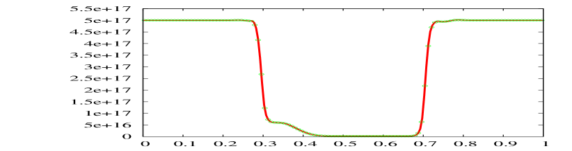
Figure 1: Density of charge in $cm^{-3}$ at $t=0.5$ ps. Continuous line ($N_{x}=200$), points ($N_{x}=120$).

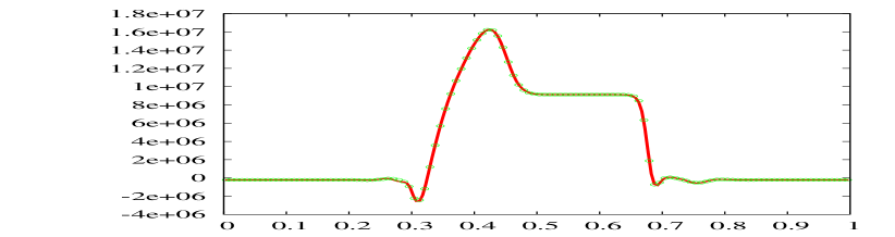
Figure 2: Velocity in $cm/s$ at $t=0.5$ ps. Continuous line ($N_{x}=200$), points ($N_{x}=120$).

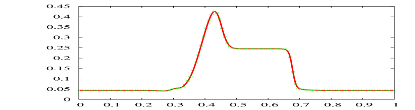
Figure 3: Mean energy in $eV$ at $t=0.5$ ps. Continuous line ($N_{x}=200$), points ($N_{x}=120$).

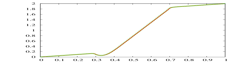
Figure 4: Electric potential in $V$ at $t=0.5$ ps. Continuous line ($N_{x}=200$), points ($N_{x}=120$).

$$\begin{array}[]{|c|c|c|}\hline\cr nx&\mbox{minimum}&\mbox{maximum}\\ \hline\cr\hline\cr 120&1.0517e-14&7.133e-04\\ \hline\cr 150&1.0517e-14&7.223e-04\\ \hline\cr 180&1.0520e-14&7.350e-04\\ \hline\cr 200&1.0519e-14&7.389e-04\\ \hline\cr\hline\cr\end{array}$$

Minimum and maximum of $pdf$ multiplied a fixed function of $\mathbf{k}$ at $0.5$ps (a.u.)

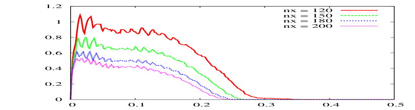
Figure 5: The ratio, multiplies by $100$, of the number of cells in phase space where $pdf$ is negative to the total numbers of cells versus time (in $ps$) for different $N_{x}$

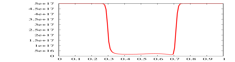
Figure 6: Density of charge in $cm^{-3}$ at $t=3.0$ ps ($N_{x}=120$).

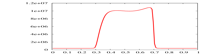
Figure 7: Velocity in $cm/s$ at $t=3.0$ ps ($N_{x}=120$).

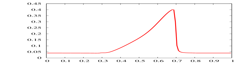
Figure 8: Mean energy in $eV$ at $t=3.0$ ps ($N_{x}=120$).

Appendix: Treatment of the transport term related to the Electric Field

The term

$$-\frac{q}{\hbar}\mathbf{E}\cdot\int_{\partial C_{\alpha}}\!\!f(t,\mathbf{x},\mathbf{k})\,\mathbf{n}\>d\sigma$$

still contains the original unknown pdf $f$, as it needs its value over the surface. However, this transport term related to the electric field $\mathbf{E}$ can be approximated by means of some standard definition of the Numerical Flux $\hat{f}$ according to the DG Method, adequate for a piecewise constant approximation. We will use the value $f_{\alpha}$ of the piecewise constant approximation for $f$ in the cell $C_{\alpha}$ and the values $f_{\gamma}$ in the nearest cells $C_{\gamma}$ neighboring $C_{\alpha}$.

To illustrate this with a particular example, consider the case in which the electric field goes along the $x$ axis: $\mathbf{E}=(E_{x},0,0)$. This 1D case has an associated cylindrical geometry in the $\mathbf{k}$-space:

$$\mathbf{k}=k_{*}(u,r\cos\theta,r\sin\theta)$$

where $k_{*}$ is a constant with dimensions of a $\mathbf{k}_{x_{i}}$-component, the normalized $u$ coordinate indicates the position along the $k_{x}$ axis, $r$ is the norm of the projection of the $\mathbf{k}$-point in a normalized $k_{y}$-$k_{z}$ plane, and $\theta\in[0,2\pi]$.

The particular symmetry of this case makes convenient to introduce annular $\mathbf{k}$-cells of the form $C_{\alpha}=[u_{a},u_{b}]\times[r_{a},r_{b}]\times[0,2\pi]$, related to the cylindrical geometry of the problem, and which look like rectangular cells on the $(u,r,\theta)$-space. Consider Figure 9, in which three neighboring $\mathbf{k}$-cells are shown: $C_{\alpha}$, $C_{\underline{\alpha}}$ (inferior to $C_{\alpha}$ in Fig. 9), and $C_{\overline{\alpha}}$ (superior to $C_{\alpha}$ in Fig. 9), as seen when projected in the $(u,r)$-space. Since in this case the 1D electric field is parallel to the $k_{x}$-axis, the transport term then reduces to:

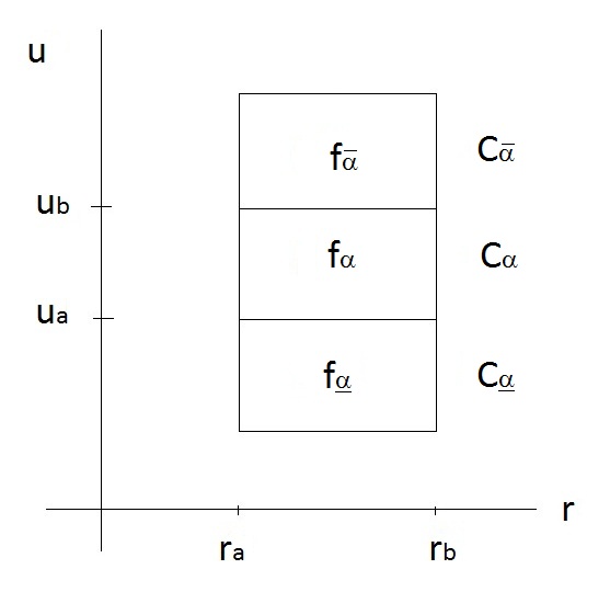
Figure 9: Cell $C_{\alpha}$, and neighbor cells $C_{\underline{\alpha}}$ (inferior) and $C_{\overline{\alpha}}$ (superior), projected in the $(u,r)$-space

$$-\frac{q}{\hbar}\mathbf{E}\cdot\int_{\partial C_{\alpha}}f(t,\mathbf{x},\mathbf{k})\,\mathbf{n}\>d\sigma\>=-\frac{q}{\hbar}E_{x}\int_{C_{\alpha}}\frac{\partial f}{\partial k_{x}}\>d\mathbf{k}$$

$$\quad=-\frac{q}{\hbar}E_{x}\>k_{*}^{2}\int_{0}^{2\pi}d\theta\int_{r_{a}}^{r_{b}}dr\int_{u_{a}}^{u_{b}}du\,\frac{\partial f}{\partial u}\>r$$

$$\quad=-\frac{q}{\hbar}E_{x}\>k_{*}^{2}\int_{0}^{2\pi}d\theta\int_{r_{a}}^{r_{b}}r\>dr\left.\left[\hat{f}(t,\mathbf{x},\mathbf{k})\right]\right|_{u_{a}}^{u_{b}}$$

For the transport term due to $-\mathbf{E}$ above, the Numerical Flux can be chosen according to the Upwind Principle. The flux over the considered boundaries is then:

$$\left.\hat{f}(t,\mathbf{x},\mathbf{k})\right|_{u=u_{a}}=\left\{\begin{array}[]{c l}f_{\alpha}(t,\mathbf{x})&\mbox{if}\quad E_{x}\geq 0,\\ f_{\underline{\alpha}}(t,\mathbf{x})&\mbox{if}\quad E_{x}<0.\end{array}\right.$$

$$\left.\hat{f}(t,\mathbf{x},\mathbf{k})\right|_{u=u_{b}}=\left\{\begin{array}[]{c l}f_{\overline{\alpha}}(t,\mathbf{x})&\mbox{if}\quad E_{x}\geq 0,\\ f_{\alpha}(t,\mathbf{x})&\mbox{if}\quad E_{x}<0.\end{array}\right.$$

References

[1]
C. Jacoboni and P. Lugli, The Monte Carlo method for semiconductor device simulation,
Spring-Verlag: Wien-New York, 1989.
[2]
Y. Cheng, I. Gamba, A. Majorana and C.-W. Shu,
A Discontinuous Galerkin solver for Boltzmann-Poisson systems
for semiconductor devices, Comput. Methods Appl. Mech. Eng.
198, 3130 (2009).