Fluctuation diagnostics of the electron self-energy: Origin of the pseudogap physics

Abstract

We demonstrate how to identify which physical processes dominate the low-energy spectral functions of correlated electron systems. We obtain an unambiguous classification through an analysis of the equation of motion for the electron self-energy in its charge, spin and particle-particle representations. Our procedure is then employed to clarify the controversial physics responsible for the appearance of the pseudogap in correlated systems. We illustrate our method by examining the attractive and repulsive Hubbard model in two-dimensions. In the latter, spin fluctuations are identified as the origin of the pseudogap, and we also explain why $d-$wave pairing fluctuations play a marginal role in suppressing the low-energy spectral weight, independent of their actual strength.

Introduction. – Correlated electron systems display some of the most fascinating phenomena in condensed matter physics, but their understanding still represents a formidable challenge for theory and experiments. For photoemission ARPESrev or STM STMrev ; STSrev spectra, which measure single-particle quantities, information about correlation is encoded in the electronic self-energy $\Sigma$. However, due to the intrinsically many-body nature of the problems, even an exact knowledge of $\Sigma$ is not sufficient for an unambiguous identification of the underlying physics. A perfect example of this is the pseudogap observed in the single-particle spectral functions of underdoped cuprates Timusk1999 , and, more recently, of their nickelate analogues Uchida2011 . Although relying on different assumptions, many theoretical approaches provide self-energy results compatible with the experimental spectra. This explains the lack of a consensus about the physical origin of the pseudogap: In the case of cuprates, the pseudogap has been attributed to spin-fluctuations spinflu1 ; spinflu2 ; spinflu3 ; spinflu4 ; spinflu5 , preformed pairs preform1 ; preform2 ; preform3 ; preform4 ; preform5 , Mottness Stanescu2003 ; Imada2013 , and, recently, to the interplay with charge fluctuations SilvaNeto2014 ; YangRice ; RiceYang ; Comin or to Fermi-liquid scenarios Mirzaei2013 . The existence and the role of ($d-$wave) superconducting fluctuations preform1 ; preform2 ; preform3 ; preform4 ; preform5 in the pseudogap regime are still openly debated for the basic model of correlated electrons, the Hubbard model.

Experimentally, the clarification of many-body physics is augmented by a simultaneous investigation at the two-particle level, i.e., via neutron scattering INSrev , infrared/optical spectroscopy OPTrev , muon-spin relaxation MUrev , etc. Analogously, theoretical studies of $\Sigma$ can also be supplemented by a corresponding analysis at the two-particle level. In this paper, we study the influence of the two-particle fluctuations on $\Sigma$ via its equation of motion. We apply this method of “fluctuation diagnostics” to identify the role played by different collective modes in the pseudogap physics.

Self-energy decomposition. – We emphasize that all concepts and equations below are applicable within any theoretical approach in which the self-energy and the two-particle vertex are calculated without a priori assumptions of a predominant type of fluctuations. This includes, e.g., quantum Monte-Carlo (QMC) methods such as lattice QMC bss , functional renormalization group fRGrev , parquet approximation parquet ; parquet1 ; Yang2009 , and cluster extensions Maier of the dynamical mean field theory (DMFT) DMFT ; DMFTrev such as the cellular-DMFT CDMFTlichtenstein ; CDMFT or the dynamical cluster approximation (DCA) DCA . Within diagrammatic extensions DGA ; DGA1 ; DF ; DF1 ; nanoDGA ; multiscale ; 1PI of DMFT, our analysis is applicable if parquet-like diagrams are included DFparquet ; DMF2RG ; nanoparquet .

The self-energy describes all scattering effects of one added/removed electron, when propagating through the lattice. In correlated electronic systems, these scattering events originate from the Coulomb interaction among the electrons themselves, rather than from the presence of an external potential. Therefore, $\Sigma$ is entirely determined by the full two-particle scattering amplitude $F$. The formal relation between $F$ and $\Sigma$ is known as Dyson-Schwinger equation of motion (EOM) Abrikosov . In the important case of a purely local interaction (as in the Hubbard model Hubbard ; Hubbard1 ; Hubbard2 ), this reads (in the paramagnetic phase)

$$\Sigma(k)=\frac{Un}{2}-\frac{U}{\beta^{2}N}\sum_{k^{\prime},q}\,F_{\uparrow\downarrow}(k,k^{\prime},q)\,g(k^{\prime})g(k^{\prime}+q)g(k+q),$$ (1)

where $U$ is the (bare) Hubbard interaction, $n$ the electronic density, $g$ the electron Green’s function, $\beta=1/T$ the inverse temperature, and $N$ the normalization of the momentum summation (we adopt the notation $k=(\nu,{\bf K})$/$q=(\omega,{\bf Q})$ for the fermionic/bosonic Matsubara frequencies $\nu$/$\omega$ and momenta ${\bf K}$/${\bf Q}$, see the supplementary material for details). Finally, $F_{\uparrow\downarrow}$ is the full scattering amplitude (vertex) between electrons with opposite spins: It consists of repeated two-particle scattering events in all possible configurations compatible with energy/momentum/spin conservation. Therefore it contains the complete information of the two-particle correlations of the system. Yet, much of the information encoded in $F_{\uparrow\downarrow}$ about the specific physical processes determining $\Sigma$ is washed out by averaging over all two-particle scattering events, i.e., by the summations on the r.h.s. of Eq. (1). Hence, an unambiguous identification of the physical role played by the underlying scattering/fluctuation processes requires a “disentanglement” of the EOM. The most obvious approach would be a direct decomposition of the full scattering amplitude $F_{\uparrow\downarrow}$ of Eq. (1) in all possible fluctuation channels, the so-called parquet parquet ; parquet1 ; parquet2 ; Yang2009 decomposition, where different contributions to $F$ are identified in terms of their two-particle reducibility. Inserting this in Eq. (1), the contributions to $\Sigma$ can be attributed to the different channels, allowing for a clear physical understanding. We find, however, that this approach only works in the weakly correlated regime (small $U$, large doping, high $T$): For stronger correlations, the numerical decomposition procedure becomes highly unstable, due to divergences in the two-particle irreducible vertex functions, recently discovered in the Hubbard and Falicov-Kimball models divergence ; unpublished ; Janis , see also Kozik2014 . For example, in our DCA calculations for the two-dimensional ($2D$) Hubbard model the breakdown of the parquet decomposition of $\Sigma$ occurs at lower values of $U$ (or larger values of doping) than those for which pseudogap physics is numerically observed.

In this paper we present an alternative route that can be followed to circumvent this problem. Our idea exploits the freedom of employing formally equivalent analytical representations of the EOM. For instance, by means of SU(2) symmetry and “crossing relations” (see, e.g., RVT ; Tam2013 ), we can express $F_{\uparrow\downarrow}$ in Eq. (1) in terms of the corresponding vertex functions of the spin/magnetic $F_{sp}=F_{\uparrow\uparrow}-F_{\uparrow\downarrow}$ and charge/density $F_{ch}=F_{\uparrow\uparrow}+F_{\uparrow\downarrow}$ sectors. Analogously, a rewriting in terms of the particle-particle sector notation is done via $F_{pp}(k,k^{\prime},q)=F_{\uparrow\downarrow}(k,k^{\prime},q-k-k^{\prime})$.

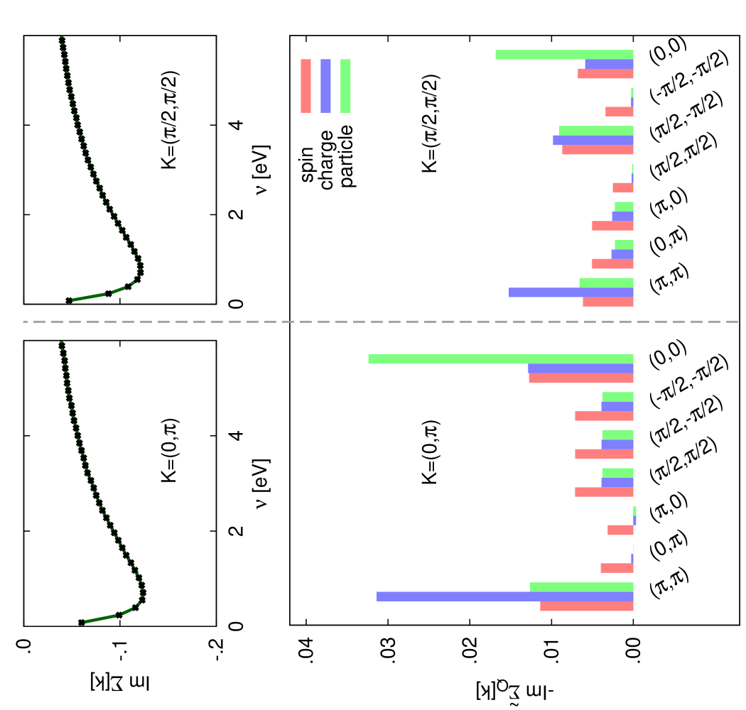
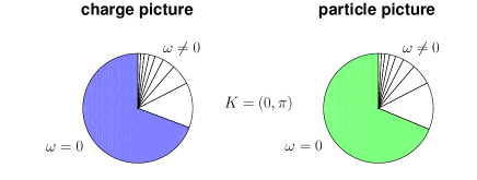
Figure 1: (Color online) Fluctuation diagnostics of Im $\Sigma({\bf K},\nu)$ (first row) for the attractive Hubbard model. The histogram shows the contributions of Im $\widetilde{\Sigma}_{\bf Q}({\bf K},\pi/\beta)$ from different values of ${\bf Q}$ in the spin, charge and particle-particle representations for the attractive 2D Hubbard model (see text). The pie charts display the relative magnitudes of $\lvert\mbox{Im}\widetilde{\Sigma}_{\omega}(\mathbf{K},\pi/\beta)\rvert$ for the first eight Matsubara frequencies $|\omega|$ in the charge and particle-particle picture, respectively.

Inserting these results in Eq. (1) and performing variable transformations, we recover Eq. (1), with $F_{\uparrow\downarrow}$ replaced by $F_{sp}$, $F_{ch}$ or $F_{pp}$. These three expressions,

$$\Sigma(k)-\Sigma_{\text{H}} =\frac{U}{\beta^{2}N}\sum_{k^{\prime},q}\,F_{sp}(k,k^{\prime};q)\,g(k^{\prime})g(k^{\prime}\!+\!q)g(k\!+\!q),$$ (2)

$$= -\,\frac{U}{\beta^{2}N}\sum_{k^{\prime},q}\,F_{ch}(k,k^{\prime};q)\,g(k^{\prime})g(k^{\prime}\!+\!q)g(k\!+\!q),$$ (3)

$$= -\,\frac{U}{\beta^{2}N}\sum_{k^{\prime},q}\,F_{pp}(k,k^{\prime};q)\,g(k^{\prime})g(q\!-\!k^{\prime})g(q\!-\!k),$$ (4)

yield the same result for $\Sigma$ after all internal summations are performed ($\Sigma_{\text{H}}$ denotes the constant Hartree term $\frac{Un}{2}$). Crucial physical insight can be gained at this stage, by performing partial summations. We can, e.g., perform all summations, except for the one over the transfer momentum Q. This gives $\widetilde{\Sigma}_{\bf Q}(k)$, i.e. the contribution to $\Sigma$ for fixed ${\bf Q}$, so that $\Sigma(k)=\sum_{\bf Q}\widetilde{\Sigma}_{\bf Q}(k)$. The vector ${\bf Q}$ corresponds to a specific spatial pattern given by the Fourier factor $e^{i\mathbf{Q}\mathbf{R}_{i}}$. For a given representation such a spatial structure is associated to a specific collective mode, e.g., ${\bf Q}\!=\!(\pi,\pi)$ for antiferromagnetic or charge-density-wave (CDW) and ${\bf Q}=(0,0)$ for superconducting or ferromagnetic fluctuations. Hence, if one of these contributions dominates, $\widetilde{\Sigma}_{\bf Q}(k)$ is strongly peaked at the ${\bf Q}$-vector of that collective mode, provided that the corresponding representation of the EOM is used. On the other hand, in a different representation, not appropriate for the dominant mode $\widetilde{\Sigma}_{\bf Q}(k)$ will display a weak ${\bf Q}$ dependence. These heuristic considerations can be formalized by expressing $F$ through its main momentum and frequency structures RVT , see Supplementary section. Hence, in cases where the impact of the different fluctuation channels on $\Sigma$ is not known a priori, the analysis of the ${\bf Q}$-dependence of $\widetilde{\Sigma}_{\bf Q}(k)$ in the alternative representations of the EOM will provide the desired diagnostics. Below, we show that this procedure works well for the cases of the 2D (attractive and repulsive) Hubbard models, allowing for an interpretation of the origin of the pseudogap phases observed there.

Results for the attractive Hubbard model. – To demonstrate the applicability of the fluctuation diagnostics, we start from a case where the underlying, dominant physics is well understood, namely the attractive Hubbard model, $U\!<\!0$ . This model captures the basic mechanisms of the BCS/Bose-Einstein crossover BCSBE ; BCSBE2 ; BCSBE3 ; BCSBE4 ; BCSBE5 and has been intensively studied both analytically and numerically, e.g., with QMC Moreo1991 ; Kyung2001 ; Paiva2004 and DMFT DMFTUneg ; DMFTUneg2 ; DMFTUneg3 ; DMFTUneg4 . Because of the local attractive interaction, the dominant collective modes are necessarily $s-$wave pairing fluctuations [${\bf Q}=(0,0)$] in the particle channel, and, for filling $n\sim 1$, CDW fluctuations [${\bf Q}=(\pi,\pi)$] in the charge channel. As we show in the following, this underlying physics is well captured by our fluctuation diagnostics.

We present here our DCA results computed on a cluster with $N_{c}=8$ sites for a 2D Hubbard model with the following parameter set: $t=-0.25$ eV, $U=-1$ eV, $\mu=-0.53$ eV and $\beta=40$ eV^-1. This leads to the occupancy $n=0.87$, for which, at this $T$, no superconducting long-range order is observed in DCA. The lower panels of Fig. 1 show the fluctuation diagnostics for $\Sigma$. The histogram depicts the different contributions to Im $\Sigma[{\bf K},\nu]$ for ${\bf K}=(0,\pi)$ and $(\pi/2,\pi/2)$ (upper panel of Fig. 1) at the lowest Matsubara frequency ($\nu=\pi/\beta$) as a function of the momentum transfer ${\bf Q}$ within the three representations [spin, charge and particle, i.e., via Eqs. (2), (3), (4)]. We observe large contributions for ${\bf Q}=(\pi,\pi)$ in the charge representation (blue bars) and for ${\bf Q}=(0,0)$ in the particle-particle representation (green bars). At the same time, no ${\bf Q}$ dominates in the spin picture. Hence, the fluctuation diagnostics correctly identifies the key role of CDW and $s-$wave pairing fluctuations in this system. This outcome is supported by a complementary analysis in frequency space (pie-chart in Fig. 1): Defining $\widetilde{\Sigma}_{\omega}(\mathbf{K},\nu)$ as contribution to the self-energy where in Eq. (1) all summations, except the one over the transfer frequency $\omega$ are performed, we observe a largely dominant contribution at $\omega=0$ ($\sim 70\%$) both in the charge and particle-particle pictures. This proves that the corresponding fluctuations are well-defined and long-lived.

Results for the repulsive Hubbard model. – We now apply the fluctuation diagnostics to the much more debated physics of the repulsive Hubbard model in 2D, focusing on the analysis of the pseudogap regime. As before, we use DCA calculations with a cluster of $N_{c}=8$ sites. $\Sigma$ and $F$ have been calculated using the Hirsch-Fye HirschFye and Continuous Time CTAUX ; CT QMC methods, accurately cross-checking the results. Specifically, we consider the parameter set $t=-0.25$ eV, $U=1.6$ eV, $\mu=0.8$ eV (corresponding to $n=1$) and $\beta=30$ eV^-1. For these parameters, the electronic self-energy (see upper panels of Fig. 2) displays strong momentum differentiation between the “antinodal” [${\bf K}=(0,\pi)$] and the “nodal” [${\bf K}=(\pi/2,\pi/2)$] momentum, with a clear pseudogap behavior at the antinode Gull2010 ; pseudogap .

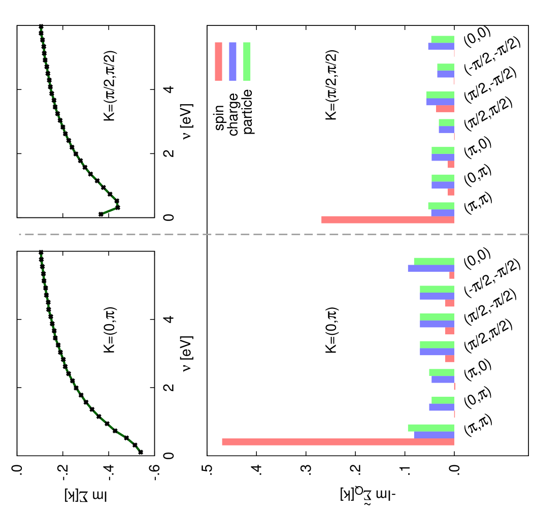
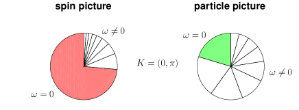
Figure 2: (Color online) As for Fig. 1: Fluctuation diagnostics of the electronic self-energy, for the case of the repulsive Hubbard model (see text).

The fluctuation diagnostics is performed in Fig. 2, where we show the contributions to Im $\Sigma[{\bf K},\pi/\beta]$ for ${\bf K}=(0,\pi)$ and $(\pi/2,\pi/2)$ (upper panels) as a function of the transfer momentum ${\bf Q}$ in the three representations. This illustrates clearly the underlying physics of the pseudogap. In the spin representation (red bars in the histogram), the ${\bf Q}=(\pi,\pi)$ contribution dominates, and contributes more than $80\%$ and $70\%$ of the result for ${\bf K}=(0,\pi)$ and ${\bf K}=(\pi/2,\pi/2)$, respectively. Conversely, all the contributions at other transfer momenta ${\bf Q}\neq(\pi,\pi)$ are about an order of magnitude smaller. The dominant ${\bf Q}=(\pi,\pi)$-contribution is also responsible for the large momentum differentiation, being almost twice as large for the antinodal self-energy. Performing the same analysis in the charge (blue bars) or particle-particle (green bars) representation, we get a completely different shape of the histogram. In both cases, the contributions to $\Sigma$ are almost uniformly distributed among all transfer momenta ${\bf Q}$.

On the basis of our previous considerations, we do not find important contributions to $\Sigma$ from charge or pairing modes, while the histogram in the spin-representation marks the strong impact of antiferromagnetic fluctuations spinflu1 ; spinflu2 ; spinflu3 ; spinflu4 ; spinflu5 ; Gull2009 ; Gull2012 . This picture is further supported by the complementary frequency analysis. The pie chart in Fig. 2 is dominated by the $\omega=0$ contribution in the spin picture, reflecting the long-lived nature of well-defined spin-fluctuations. At the same time, in the particle (and charge, not shown) representation, the contributions are more uniformly distributed among all $\omega$’s, which corresponds to short-lived pairing (charge) fluctuations.

Physical interpretation of the pseudogap.– We are now in the position to draw some general conclusions on the physics underlying a pseudogap. These considerations are relevant for the underdoped cuprates, up to the extent their low-energy physics is captured by the $8$-site DCA for the repulsive 2D Hubbard model. For simplicity, we focus here on our data for the unfrustrated model at half-filling, which exhibits a pseudogap in the parameter regime considered. By means of fluctuations diagnostics we identify a well-defined [$\mathbf{Q}\!=\!(\pi,\pi)$] collective spin-mode to be responsible (on the 75% level) both for the momentum differentiation of $\Sigma$ and for its pseudogap behavior at the antinode: The large values of $\widetilde{\Sigma}_{\mathbf{Q}}$ at $\mathbf{Q}\!=\!(\pi,\pi)$ and $\widetilde{\Sigma}_{\omega}$ at $\omega=0$ are the distinctive hallmark of long-lived and extended (antiferromagnetic) spin-fluctuations. At the same time, the rather uniform $\mathbf{Q}$- and $\omega$-distribution of $\widetilde{\Sigma}_{\mathbf{Q}}$ and $\widetilde{\Sigma}_{\omega}$ in the charge/particle pictures shows that the well-defined spin mode can be also viewed as short-lived and short-range charge/pair fluctuations. The latter cannot be interpreted, hence, in terms of preformed pairs. This scenario for the pseudogap matches very well the different estimates of fluctuation strengths in previous DCA studies pseudogap ; pseudogap1 ; Gull2012 . We also emphasize the general applicability of our result (see Supplementary): A well defined mode in one channel appears as short-lived fluctuations in other channels. This dichotomy is not visible anymore in $\Sigma$, which makes our fluctuations diagnostics a powerful tool for identifying the most convenient viewpoint to understand the physics responsible of the observed spectral properties.

Let us finally turn our attention to the still open question about the impact of superconducting $d$-wave fluctuations on the normal-state spectra in the pseudogap regime of the Hubbard model. The instantaneous fluctuations are defined as $\langle\Delta_{d}^{\dagger}\Delta_{d}\rangle$, with $\Delta_{d}^{\dagger}=\sum_{\bf K}f({\bf K})c^{\dagger}_{{\bf K}\uparrow}c^{\dagger}_{-{\bf K}\downarrow}$ and $f({\bf K})={\rm cos}K_{x}-{\rm cos}K_{y}$. These ${\bf Q}=0$ fluctuations are certainly strong in proximity of the superconducting phase, but they were also foundpseudogap to be significant over short distances in the pseudogap regime. Their intensity gets stronger as $U$ is increased, beyond the values where superconductivity exists. The expression for $\tilde{\Sigma}_{{\bf Q}=(0,0)}$ in the particle picture is closely related to $\langle\Delta_{d}^{\dagger}\Delta_{d}\rangle$, except that the factor $f({\bf K})$ is missing in $\tilde{\Sigma}_{\bf Q}$ (see Supplementary). One might therefore have expected that large ${\bf Q=0}$ pair fluctuations, irrespectively of their lifetime, would have contributed strongly to $\Sigma$. For unconventional superconductivity, e.g., $d-$wave, this does not happen. The reason is the angular variation of $f({\bf K})$. For strong pair fluctuations, the variations of $f({\bf K})$ make the contributions to the fluctuations add up, while the contributions to $\Sigma$ then tend to cancel. This explains why suppressing superconductivity fluctuations pseudogap ; pseudogap1 ; Vilk1997 ; Sigmak ; DF1 ; DGA1 ; DGA2 ; Avella2014 does not affect the description of the pseudogap of the Hubbard model. In the case of a purely local interaction such as in the EOM like Eq. (1), enhanced $\langle\Delta_{d}^{\dagger}\Delta_{d}\rangle$ fluctuations are mostly averaged out by the momentum summation (see Supplementary).

Conclusions. – We have shown that if a simultaneous calculation of the self-energy and the vertex functions is performed, it is possible to identify the impact of the different collective modes on the spectra of correlated systems (“fluctuation diagnostics”). This is achieved by expressing the equation of motion for $\Sigma$ in different representations (e.g., spin/charge/particle), which avoids all the intrinsic instabilities of parquet decompositions. We apply this procedure to the $U<0$ and $U>0$ 2D Hubbard model. In the attractive case we have confirmed the dominant role of pair fluctuations, supporting the validity of our approach. For the repulsive model, relevant for the physics of the underdoped cuprates, spin fluctuations emerged as mainly responsible for the spectral function results, in agreement with other studies spinflu1 ; spinflu2 ; spinflu3 ; spinflu4 ; spinflu5 ; Gull2012 . The same well-defined spin modes might appear, on a different perspective, as strong, but rapidly decaying, pair fluctuations. Finally, for a purely local interaction, $d-$wave pairing fluctuations will only weakly affect the pseudogap spectral properties even on the verge of the superconducting transition.

These results, as well as the insight on the pseudogap physics, suggest that fluctuation diagnostics can be broadly used in future studies. The progress in calculating vertex functions Gunnarsson2010 ; RVT ; Hafermann2014 will allow its applicability also to other, more complex, multi-orbital models LDACDMFT1 ; LDAVCA ; LDACDMFT2 ; LDADCA ; abinitioDGA ; LDAFRG ; multiDCA : Here, due to the increased number of degrees of freedom, the identification of the dominant fluctuation mode(s) will be of the utmost importance for a correct physical understanding.

Acknowledgments. – We thank A. Tagliavini, C. Taranto, S. Andergassen, and M. Capone for insightful discussions. We acknowledge support from the FWF through the PhD School “Building Solids for Function” (TS, Proj. Nr. W1243) and the project I-610 (GR, AT), from the research unit FOR 1346 of the DFG (GS), from MINECO: MAT2012-37263-C02-01 (JM), and from the Simons foundation (JPFL,EG). GS and AT also acknowledge the hospitality in Campello sul Clitunno.

References

- (1) A. Damascelli, Z. Hussain, and Zhi-Xun Shen, Rev. Mod. Phys. 75, 473 (2003).
- (2) G. Binnig and H. Rohrer, Rev. Mod. Phys. 59, 615 (1987).
- (3) O. Fischer, M. Kugler, I. Maggio-Aprile, C. Berthod, and Christoph Renner, Rev. Mod. Phys. 79, 353 (2007).
- (4) T. Timusk and B. W. Statt, Rep. Prog. Phys. 62, 61 (1999).
- (5) M. Uchida et al., Phys. Rev. Lett. 106, 027001 (2011).
- (6) D. J. Scalapino, Rev. Mod. Phys. 84, 1383 (2012).
- (7) C. Huscroft, M. Jarrell, Th. Maier, S. Moukouri, and A.N. Tahvildarzadeh, Phys. Rev. Lett. 86, 139 (2001).
- (8) D. Sénéchal and A.M.S. Tremblay, Phys. Rev. Lett. 92, 126401 (2004).
- (9) B. Kyung, S. S. Kancharla, D. Senechal, A.M.S. Tremblay, M. Civelli, and G. Kotliar, Phys. Rev. B 73, 165114 (2006).
- (10) A. Macridin, M. Jarrell, T. Maier, P.R.C. Kent, and E. D’Azevedo, Phys. Rev. Lett. 97, 036401 (2006).
- (11) V.J. Emery and S.A. Kivelson, Nature 374, 434 (1995).
- (12) Z. A. Xu, N. P. Ong, Y. Wang T. Kakeshita, and S. Uchida, Nature 406, 486 (2000).
- (13) Y. Wang, L. Li, M. J. Naughton, G. D. Gu, S. Uchida, and N. P. Ong, Phys. Rev. Lett. 95, 247002 (2005).
- (14) Y. Kosaka, T. Hanaguri, M. Azuma, M. Takano, J. C. Davis, and H. Takagi, Nature Physics 8, 534 (2012).
- (15) M. Norman, Nature Physics, 10 357 (2014).
- (16) T. D. Stanescu and P. Phillips, Phys. Rev. Lett. 91 017002 (2003).
- (17) M. Imada, S. Sakai, Y. Yamaji, and Y. Motome, J. Phys.: Conf. Ser. 449 012005 (2013).
- (18) E. H. da Silva Neto, P. Aynajian, A. Frano, R. Comin, E. Schierle, E. Weschke, A. Gyenis, J. Wen, J. Schneeloch, Z. Xu, S. Ono, G. Gu, M. Le Tacon, and A. Yazdani, Science 343, 393 (2014).
- (19) K.-Y. Yang, T. M. Rice, and R. C. Zhang, Phys. Rev. B 73, 174501 (2006).
- (20) T. M. Rice, K.-Y. Yang, and F. C. Zhang, Rep. Prog. Phys. 75, 016502 (2012).
- (21) R. Comin, et al., Science, 343, 390 (2013).
- (22) S. I. Mirzaei, D. Strickera, J. N. Hancocka, C. Berthoda, A. Georges, Erik van Heumen, M. K. Chan, X. Zhao, Y. Li, M. Greven, N. Barisiĉ, and D. van der Marel, PNAS 110, 5774 (2012).
- (23) R. J. Birgeneau, C. Stock, J. M. Tranquada, and K. Yamada, J. Phys. Soc. Jpn. 75, 111003 (2006).
- (24) D. N. Basov and T. Timusk, Rev. Mod. Phys. 77, 721 (2006).
- (25) J. Sonier, J. Brewer, and R. Kiefl, Rev. Mod. Phys. 72, 769 (2000).
- (26) R. Blankenbecler, D. J. Scalapino, and R. L. Sugar, Phys. Rev. D 24, 2278 (1981).
- (27) W. Metzner, M. Salmhofer, C. Honerkamp, V. Meden, and K. Schönhammer, Rev. Mod. Phys. 84, 299 (2012).
- (28) N. E. Bickers, D. J. Scalapino, and S. R. White, Phys. Rev. Lett. 62, 961 (1989).
- (29) V. Janiŝ, J. Phys.: Condens. Matter 10, 2915 (1998); Phys. Rev. B 60, 11345 (1999).
- (30) S.X. Yang, H. Fotso, J. Liu, T. A. Maier, K. Tomko, E. F. D’Azevedo, R. T. Scalettar, T. Pruschke, and M. Jarrell, Phys. Rev. E 80, 046706 (2009).
- (31) T. Maier, M. Jarrell, T. Pruschke, and M. H. Hettler, Rev. Mod. Phys. 77, 1027 (2005).
- (32) W. Metzner and D. Vollhardt, Phys. Rev. Lett. 62, 324 (1989).
- (33) A. Georges, G. Kotliar, W. Krauth, and M. Rozenberg, Rev. Mod. Phys. 68, 13 (1996).
- (34) A. I. Lichtenstein and M. I. Katsnelson, Phys. Rev. B 62, R9283 (2000).
- (35) G. Kotliar, S.Y. Savrasov, G. Pálasson, and G. Biroli, Phys. Rev. Lett. 87, 186401 (2001).
- (36) M. H. Hettler, M. Mukherjee, M. Jarrell, and H. R. Krishnamurthy, Phys. Rev. B 61, 12739 (2000).
- (37) A. Toschi, A. A. Katanin, and K. Held, Phys. Rev. B 75, 045118 (2007).
- (38) K. Held, A. A. Katanin, and A. Toschi, Prog. Theor. Phys. Suppl. 176, 117 (2008).
- (39) A. N. Rubtsov, M. I. Katsnelson, and A. I. Lichtenstein, Phys. Rev. B 77, 033101 (2008).
- (40) H. Hafermann, G. Li, A. N. Rubtsov, M. I. Katsnelson, A. I. Lichtenstein, and H. Monien, Phys. Rev. Lett. 102, 206401 (2009).
- (41) C. Slezak, M. Jarrell, Th. Maier, and J. Deisz, J. Phys.: Condens. Matter 21, 435604 (2009).
- (42) A. Valli, G. Sangiovanni, O. Gunnarsson, A. Toschi, and K. Held, Phys. Rev. Lett. 104 246402 (2010).
- (43) G. Rohringer, A. Toschi, H. Hafermann, K. Held, V. I. Anisimov, and A. A. Katanin, Phys. Rev. B 88, 115112 (2013).
- (44) S.-X. Yang, H. Fotso, H. Hafermann, K.-M. Tam, J. Moreno, T. Pruschke, and M. Jarrell, Phys. Rev. B 84, 155106 (2011).
- (45) C. Taranto, S. Andergassen, J. Bauer, K. Held, A. Katanin, W. Metzner, G. Rohringer, and A. Toschi, Phys. Rev. Lett. 112, 196402 (2014).
- (46) A Valli, T Schäfer, P Thunström, G Rohringer, S Andergassen, G Sangiovanni, K Held, and A Toschi, arXiv:1410.4733.
- (47) A. A. Abrikosov et al., Methods of Quantum Field Theory in Statistical Physics (Dover, New York, 1963).
- (48) J. Hubbard, Proc. Roy. Soc. London A 276, 238 (1963).
- (49) M. C. Gutzwiller, Phys. Rev. Lett. 10, 159 (1963).
- (50) J. Kanamori, Progr. Theor. Phy. 30, 275 (1963).
- (51) D. Senechal et al., Theoretical Methods for Strongly Correlated Electrons (Springer, Berlin, 2003), Chapter 6.
- (52) T. Schäfer, G. Rohringer, O. Gunnarsson, S. Ciuchi, G. Sangiovanni, and A. Toschi, Phys. Rev. Lett. 110, 246405 (2013).
- (53) see unpublished appendix of DFparquet in arXiv:1104.3854v1.
- (54) V. Janiš and V. Pokorný, Phys. Rev. B 90, 045143 (2014).
- (55) E. Kozik, M. Ferrero, and A. Georges, arXiv:1407.5687.
- (56) G. Rohringer, A. Valli, and A. Toschi, Phys. Rev. B 86, 125114 (2012).
- (57) K.M. Tam, H. Fotso, S.X. H. Yang, and T.W. Lee, J. Moreno, J. Ramanujam, and M. Jarrell, Phys. Rev. E, 87, 013311 (2013).
- (58) R. Micnas, J. Ranninger, and S. Robaszkiewicz, Rev. Mod. Phys. 62, 113 (1990).
- (59) Sà de Melo, M. Randeria, and J. R. Engelbrecht, Phys. Rev. Lett. 71, 3202 (1993).
- (60) R. Haussmann, Z. Phys. B 91, 291 (1993).
- (61) F. Pistolesi and G. C. Strinati, Phys. Rev. B 53, 15168 (1996).
- (62) B. Kyung, S. Allen, and A.-M. S. Tremblay, ibid. 64, 075116 (2001).
- (63) A. Moreo and D. J. Scalapino, Phys. Rev. Lett. 66, 946 (1991).
- (64) B. Kyung, S. Allen, and A.-M. S. Tremblay, Phys. Rev. B 64, 075116 (2001).
- (65) T. Paiva, R. R. dos Santos, R. T. Scalettar, and P. J. H. Denteneer, Phys. Rev. B 69, 184501 (2004).
- (66) M. Keller, W. Metzner, and U. Schollwöck, Phys. Rev. Lett. 86, 4612 (2001).
- (67) A. Toschi, P. Barone, M. Capone, and C. Castellani, New J. Phys. 7, 7 (2005).
- (68) A. Toschi, M. Capone, and C. Castellani, Phys. Rev. B 72, 235118 (2005).
- (69) A. Garg, H. R. Krishnamurthy, and M. Randeria, Phys. Rev. B 72, 024517 (2005).
- (70) J. E. Hirsch and R. M. Fye, Phys. Rev. Lett. 56, 2521 (1986).
- (71) E. Gull, P. Werner, O. Parcollet, and M. Troyer, Eur. Phys. Lett. 82, 57003 (2008).
- (72) E. Gull, A. J. Millis, A. I. Lichtenstein, A. N. Rubtsov, M. Troyer, and P. Werner, Rev. Mod. Phys. 83, 349 (2011).
- (73) E. Gull, O. Parcollet, P. Werner, and A.J. Millis, Phys. Rev. B 82, 155101 (2010).
- (74) J. Merino and O. Gunnarsson, Phys. Rev. B 89, 245130 (2014); see also: arXiv:1310.4597.
- (75) E. Gull, O. Parcollet, P. Werner, and A.J. Millis, Phys. Rev. B 80, 245102 (2009).
- (76) E. Gull and A. J. Millis, Phys. Rev. B 86, 2411106(R) (2012)
- (77) J. Merino and O. Gunnarsson, J. Phys.: Cond. Matter. 25, 052201 (2013).
- (78) Y.M. Vilk and A.M.S.Tremblay, J. Phys. I 7, 1309 (1997).
- (79) E. Z. Kuchinskii, I. A. Nekrasov, and M. V. Sadovskii, Sov. Phys. JETP Lett. 82, 98 (2005).
- (80) A.A. Katanin, A. Toschi, and K. Held, Phys, Rev. B 80, 075104 (2009).
- (81) A. Avella, Adv. Cond. Matt. Phys. 2014, 515698 (2014).
- (82) O. Gunnarsson, G. Sangiovanni, A. Valli, and M. W. Haverkort, Phys. Rev. B 82, 233104 (2010).
- (83) H. Hafermann, Phys. Rev. B 89, 235128 (2014).
- (84) S. Biermann, A. Poteryaev, A. I. Lichtenstein, and A. Georges, Phys. Rev. Lett. 94, 026404 (2005).
- (85) T. Saha-Dasgupta, S. Glawion, M. Sing, R. Claessen, and R.Valentí, New J. Phys. 9, 380 (2007).
- (86) J. M. Tomczak, F. Aryasetiawan, and S. Biermann, Phys. Rev. B 78, 115103 (2008).
- (87) M. Aichhorn, T. Saha-Dasgupta, R. Valentí, S. Glawion, M. Sing, and R. Claessen, Phys. Rev. B 80, 115129 (2009).
- (88) A. Toschi, G. Rohringer, A. A. Katanin, and K. Held, Annalen der Physik 523, 698 (2011).
- (89) C. Platt, W. Hanke, and R. Thomale, Adv. Phys. 62, 453 (2013).
- (90) Y. Nomura, S. Sakai, and R. Arita, Phys. Rev. B 89, 195146 (2014).