Euclidean Dynamical Symmetry in Nuclear Shape Phase Transitions

Abstract

The Euclidean dynamical symmetry hidden in the critical region of nuclear shape phase transitions is revealed by a novel algebraic F(5) description. With a nonlinear projection, it is shown that the dynamics in the critical region of the spherical–axial deformed and the spherical–$\gamma$ soft shape phase transitions can indeed be manifested by this description, which thus provides a unified symmetry–based interpretation of the critical phenomena in the region.

Dynamical symmetries (DSs) play an important role in elucidating the quintessential nature of quantum many-body dynamical structures, especially their evolution under changing conditions. Typical examples of DS are those associated with the interacting boson model (IBM) IachelloBook87 for nuclear structure and the vibron model (VM) IachelloBook95 for molecules and atomic clusters HJP2006 , where various DSs provide considerable insight into the nature of shape phases and shape phase transitions (SPTs) Cejnar2010 .

The IBM possesses an overall U(6) symmetry with three DSs corresponding to three special nuclear shapes or collective modes; namely, a spherical vibrator [U(5)], an axially deformed rotor [SU(3)], and a $\gamma$-soft rotor [O(6)] ICSM-Initial ; ICSM-Rot . In nuclei, the typical shape phase diagram can be characterized by the so-called Casten triangle Casten2007 in the IBM parameter space with the three DSs placed at the vertices of the triangle as shown in Fig. 1. Experimental observations show not only that these three DSs indeed exist in nuclei, but also the SPTs occur with two good examples IachelloBook87 being the first-order SPT from U(5) to SU(3) and the second-order SPT from U(5) to O(6). Additionally, quasidynamical symmetries have been found to occur along the legs of the Casten triangle Rowe2004 and even inside the triangle Bonatsos2010 . It has been also shown that partial dynamical symmetries may occur at the critical point of a SPT Leviatan2007 . On the other hand, within the Bohr-Mottelson Model (BMM) Bohr1998 , the E(5) Iachello2000 ; Caprio2007 and X(5) Iachello2001 critical point symmetries (CPSs) were developed to approximately but analytically describe the states at the critical point of the spherical to $\gamma$-soft SPT and those of the spherical to axially deformed SPT, respectively. Accordingly, the structural paradigms in the triangle shown in Fig. 1 can also be labelled with the BMM language of vibrator, (axial) rotor, $\gamma$-soft (rotor), E(5) and X(5), which are the solutions to the Bohr Hamiltonian. However, the distinction between the IBM and the BMM should be borne in mind. Then the algebraic collective model was developed to provide a computationally tractable version of the BMM ACM1 . However, the DS structure of the CPSs is still lacking. In this work, we will make clear the dynamical structure of the CPSs, and establish the approach to describe the states in the transitional region connecting the two critical point symmetries as shown in Fig. 1 in a unified way.

The E(5) CPS was initiated with the solution of the five-dimensional square well potential in the BMM, and the corresponding Hamiltonian is invariant under both translations and rotations in five-dimensional space if confined in the well. It holds then the five-dimensional Euclidean symmetry, the Eu(5) symmetry Caprio2007 . By implementing $d$-boson creation and annihilation operators for the five-dimensional system with

$$\tilde{d}_{u}=\frac{1}{\sqrt{2}}\left[q_{u}+i\tilde{p}_{u}\right],~{}~{}~{}~{}d^{{\dagger}}_{u}=\frac{1}{\sqrt{2}}\left[q_{u}-i\tilde{p}_{u}\right]\,,$$ (1)

where $q_{u}$ and $\tilde{p}_{u}$ are the coordinates and the associated momenta in spherical tensor form Marshalek2006 ; Klein1982 with $\tilde{A}_{u}=(-)^{u}A_{-u}$, and using the definition of Casimir operator of the Eu(5) group, $C_{2,\textrm{\footnotesize{Eu(5)}}}=\tilde{p}^{2}$ (see, for example, Ref. Caprio2007 ), one can give the algebraic Hamiltonian with the Eu(5) DS,

$$\hat{H}_{\rm F(5)}=\alpha[\hat{n}_{d}+\frac{5}{2}-\frac{1}{2}\left(\hat{P}^{{\dagger}}_{d}+\hat{P}_{d}\right)]\,,$$ (2)

where $\alpha$ is a scale factor, $\hat{n}_{d}=\sum_{u}d^{{\dagger}}_{u}d_{u}$ and $\hat{P}_{d}=\sum_{u}(-)^{u}d_{u}d_{-u}$. The Hamiltonian (2) can be diagonalized PD under the $\mathrm{U(5)}\supset\mathrm{O(5)}\supset\mathrm{O(3)}$ basis $\{|n_{d}\,\tau\;\Delta\,L\rangle\}$ with $0\leq n_{d}<\infty$. It should be noted that this scheme does not lie in the framework of the IBM due to the non-compactness of the Eu(5) group, but can be translated directly from the geometric description of the E(5) CPS Iachello2000 because the Hamiltonian of the latter may be written as $\hat{H}_{\rm BMM}=\frac{1}{2B}\tilde{p}^{2}=\frac{1}{2B}C_{2,\textrm{\footnotesize{Eu(5)}}}$, which, however, should be confined within an infinite square well Caprio2007 . Besides, it is not easy to include the boundary condition of the square well directly in the algebraic realization when diagonalizing the Hamiltonian (2). Owing to the fact that the boson number $N$ is fixed in the IBM, if the $d$-bosons constructed in (1) are regarded to be equivalent to those in the IBM, practical calculation with the algebraic Eu(5) Hamiltonian (2) can be realized by diagonalizing the corresponding IBM analogue within the U(6) subspace for fixed boson number $N$. We refer it then to the F(5) scheme. One can verify numerically that ratios of the eigen-energies and the eigenstates of an infinite well problem can indeed be produced approximately by diagonalizing the Hamiltonian (2) within a finite boson subspace. The larger the boson number $N$, the better the approximation. Thus, the link between the geometric and the dynamical F(5) algebraic description of the CPS in the critical region of the SPT is established.

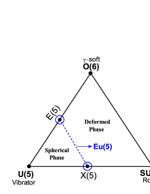
Figure 1: (Color online) Nuclear shape phase diagram characterized by the symmetry triangle. Note that there are two systems for labeling this paradigm; the geometric language and the IBM (see the text).

Table 1: Typical energy and $B(E2)$ ratios in the F(5) scheme with different $\chi$ at $N=1000$ together with those in the related models.

	E(5)	F(5) at $N=1000$						X(5)	U(5)	O(6)	SU(3)
		$\chi=0.0$	$\chi=-0.4$	$\chi=-0.8$	$\chi=-1.0$	$\chi=-1.1$	$\chi=-1.32$
$E_{4_{1}}/E_{2_{1}}$	2.20	2.19	2.33	2.51	2.63	2.71	2.89	2.91	2.00	2.50	3.33
$E_{6_{1}}/E_{0_{2}}$	1.18	1.19	1.12	1.05	1.01	1.00	0.96	0.96	1.50	1.00	$\frac{21}{8N-4}$
$E_{0_{2}}/E_{2_{1}}$	3.03	3.02	3.53	4.22	4.67	4.93	5.61	5.67	2.00	4.50	$\frac{4(2N-1)}{3}$
$\frac{B(E2;~{}4_{1}\rightarrow 2_{1})}{B(E2;~{}2_{1}\rightarrow 0_{1})}$	1.68	1.67	1.65	1.63	1.62	1.61	1.60	1.58	$\frac{2(N-1)}{N}$	$\frac{10(N^{2}+4N-5)}{7(N^{2}+4N)}$	$\frac{10(4N^{2}+6N-10)}{7(4N^{2}+6N)}$
$\frac{B(E2;~{}0_{2}\rightarrow 2_{1})}{B(E2;~{}2_{1}\rightarrow 0_{1})}$	0.86	0.86	0.79	0.72	0.68	0.66	0.62	0.63	$\frac{2(N-1)}{N}$	0.00	0.00

The E(5) and X(5) models are both restricted to an infinite square well potential in $\beta$, the only difference between the two models is how the $\gamma$ degree of freedom is handled Iachello2000 ; Iachello2001 . If only $n_{\gamma}=0$ states in the X(5) model Iachello2001 are considered, which corresponds to the yrast and yrare states, the $\beta$ dependence in the E(5) and X(5) models can be expressed uniformly by the Bessel equation:

$$\psi^{\prime\prime}(z)+\frac{\psi^{\prime}(z)}{z}+\left(1-\frac{v^{2}}{z^{2}}\right)\psi(z)=0\,,$$ (3)

where $\psi(z)\sim z^{-3/2}J_{v}(z)$ with $J_{v}(z)$ being a Bessel function of order $v$, in which $z$ is proportional to the $\beta$ variable. For the E(5) model, $v=\tau+3/2$ with $\tau$ being the seniority number of the O(5) group, while for the X(5) model, $v=\left[\frac{L(L+1)}{3}+\frac{9}{4}\right]^{1/2}$ with $L$ being the angular momentum quantum number. Accordingly, we can establish a mapping $v=f(L,\chi)$ with $f(L,0)=\tau$ since $L=2\tau$ for the yrast states in this case and $f(L,-\frac{\sqrt{7}}{2})=\left[\frac{L(L+1)}{3}+\frac{9}{4}\right]^{1/2}$. Obviously, there are many different choices for $f$, but since they are homotopic to one and another, each one should then correspond to a way to get those from the E(5) critical point to the X(5) critical point. For simplicity, we take the linear mapping

$$v=\left(1\!+\!\frac{2}{\sqrt{7}}\chi\right)\frac{L}{2}-\frac{2\chi}{\sqrt{7}}\left[\frac{-3\!+\!\sqrt{9\!+\!4L(L\!+\!1)/3}}{2}\right]+\frac{3}{2}\,$$ (4)

with $\chi\in[0,-\frac{\sqrt{7}}{2}]$. For a given $\chi$, we define a projection $\hat{P}_{\tau^{\prime},\tau}^{\chi}$ that projects the quantum number $\tau$ to be equivalent to $\tau^{\prime}=\nu-3/2$ according to (4). Obviously, the projection is nonlinear because of the nonlinear dependence of $\nu$ on the quantum number $L$ ($\tau$) shown in (4). We found that, after the projection, the Hamiltonian given in (5) can be rewritten in terms of functionals of the U(5) operators with

$$\!\!\!\!\hat{H}^{\prime}_{\rm F(5)}=(\hat{P}_{\tau^{\prime},\tau}^{\chi})^{\dagger}\hat{H}_{\rm F(5)}\hat{P}_{\tau^{\prime},\tau}^{\chi}=$$

$$\;\;A+\frac{2\chi}{\sqrt{7}}\sqrt{B}-\frac{\chi}{\sqrt{7}}\sqrt{\frac{16}{3}B-\frac{40}{3}\sqrt{B}+17}+\frac{5}{2}$$

$$\;\;-\frac{A+(1+\frac{4\chi}{\sqrt{7}})\sqrt{B}-\frac{2\chi}{\sqrt{7}}\sqrt{\frac{16}{3}B-\frac{40}{3}\sqrt{B}+17}+\frac{7}{2}}{2(A+\sqrt{B}+\frac{7}{2})}~{}C^{\dagger}$$

$$\;\;-~{}C\frac{A+(1+\frac{4\chi}{\sqrt{7}})\sqrt{B}-\frac{2\chi}{\sqrt{7}}\sqrt{\frac{16}{3}B-\frac{40}{3}\sqrt{B}+17}+\frac{7}{2}}{2(A+\sqrt{B}+\frac{7}{2})},\;\;\;$$ (5)

where $A=\hat{n}_{d}$, $B=\hat{n}_{d}(\hat{n}_{d}+3)-2P_{d}^{\dagger}P_{d}+\frac{9}{4}$, $C=P_{d}$, and the scale factor in (2) has been set as $\alpha=1$. The expression (Euclidean Dynamical Symmetry in Nuclear Shape Phase Transitions) is the Hamiltonian for $\chi\in[0,-\frac{\sqrt{7}}{2}]$, which is well defined when being diagonalized under the $\mathrm{U(6)}\supset\mathrm{U(5)}\supset\mathrm{O(5)}\supset\mathrm{O(3)}$ basis, and regains the Hamiltonian (2) as taking $\chi=0$. The quadrupole operator in this case may be taken simply as $T_{u}=e(d^{\dagger}+\tilde{d})_{u}^{(2)}$ with $e$ being an effective charge. As a result, a symmetry-based realization of the dynamical structural evolution between the E(5) and the X(5) CPSs is provided in the F(5) scheme.

Several typical energy and $B(E2)$ ratios in the related models are listed in Table 1. The results show clearly that the F(5) scheme with $\chi=0$ and $\chi=-1.32$ in the large $N$ limit reproduces nicely the results of the E(5) and X(5) models. Furthermore, the calculated quantities increase or decrease monotonously as $\chi$ changes from the X(5) limit with $\chi\approx-1.32$ to the E(5) limit with $\chi=0$, which all fall between those of the spherical vibrator [U(5)] and the deformed rotor [O(6), SU(3), or O(6) and SU(3) mixed for some cases]. The results indicate that the Eu(5) DS can definitely be considered as the critical DS of the spherical to deformed SPT region as shown in Fig. 1.

It is remarkable that the bandhead energies of excited $0^{+}$ states for any given $N$ in the F(5) scheme are universally independent of $\chi$ when normalized to $E_{0_{2}}$. For example, $E_{0_{3}}/E_{0_{2}}=2.57$ for $N=10$ and $E_{0_{3}}/E_{0_{2}}=2.50$ for $N=1000$, which in the large $N$ limit coincides with the rule of $E_{0_{n}}=A(n-1)(n+2)$ Bonatsos2008II , where $A$ is a $\chi$-dependent parameter. The analysis in Ref. Bonatsos2008II shows that the same law also occurs to the excited $0^{+}$ states around the critical point of the U(5)–SU(3) SPT in the large $N$ limit. Similarly, energies of the excited $14^{+}$ states in the F(5) scheme are also independent of $\chi$ for any given $N$. This can be easily explained based on (4), in which the values of $v$ for $L=0$ and $L=14$ are independent of $\chi$ and given by $v=\frac{3}{2}$ and $v=\frac{17}{2}$, respectively. As a result, the ratio $E_{14_{1}}/E_{0_{2}}$ can be taken as a signal of the Eu(5) DS occurring in even-even nuclei. Furthermore, as shown in Table 1, energies of the $6^{+}_{1}$ and $0^{+}_{2}$ states in the F(5) scheme with $-1.32\leq\chi\leq-0.8$ are approximately degenerate in the large $N$ limit. Detailed calculations indicate that the approximate degenerate situations also occur among other states, e.g., ($10^{+}_{1}$, $0^{+}_{3}$), ($14^{+}_{1}$, $0^{+}_{4}$), and so on, but the degeneracies are gradually removed with increasing excitation energies. As discussed in Ref. Bonatsos2008 , the degeneracies of ($6^{+}_{1}$, $0^{+}_{2}$), etc, are the signature of the underlying symmetry within the critical region in the large $N$ limit. These numerical results demonstrate further that the underlying symmetry can be attributed to the Eu(5) DS at least for low-lying states. Moreover, the experimental data of some typical quantities for the transitional nuclei Cejnar2010 ; Casten2007 previously identified as the candidates of either the E(5) Iachello2000 or X(5) CPS Iachello2001 , together with those calculated from Eq. (Euclidean Dynamical Symmetry in Nuclear Shape Phase Transitions), are shown in Table 2. One can observe from Table 2 that the experimental data are well fitted by the F(5) scheme except for the inter-band $B(E2)$ ratio shown in the last row. A possible improvements in the theoretical prediction about the inter-band $B(E2)$ ratio may be made by adding additional terms such as $(d^{\dagger}\tilde{d})_{u}^{(2)}$ in the quadrupole operator based on the analysis in Arias2001 . More specifically, the approximate degeneracy of the $6^{+}_{1}$–$0^{+}_{2}$ levels emerges clearly both in experiment and in the F(5) scheme for the cases with large $|\chi|$ value, and the constant value of $E_{14_{1}}/E_{0_{\xi}}$ predicted by the theory is also confirmed by experiment, which indicates that these critical nuclei may be possible candidates for the Eu(5) symmetry.

Table 2: Some typical energy and $B(E2)$ ratios for ¹⁰²Pd Frenne9809 ; Zamfir2002 , ¹²⁸Xe Kanbe2001 ; Coquard2009 , ^146,148Ce Peker1997 ; Bhat2000 , and ¹⁵⁰Nd Basu2013 , together with those calculated from Eq. (Euclidean Dynamical Symmetry in Nuclear Shape Phase Transitions) with different $\chi$ at $N=1000$, where “$-$” denotes the quantities undetermined in experiment. (N.B., the $0_{\xi}$ state represents the band head state of the $\xi=2$ family as that in the E(5) CPS description.)

Ratio			($\chi$, nucleus)
	($-0.2$,102Pd)	($-0.4$,128Xe)	($-0.9$,146Ce)	($-1.2$,148Ce)	($-1.3$,150Nd)
$E_{4_{1}}/E_{2_{1}}$	(2.26,  2.29)	(2.33,  2.33)	(2.57,  2.58)	(2.78,  2.86)	(2.89,  2.93)
$E_{6_{1}}/E_{2_{1}}$	(3.75,  3.79)	(3.94,  3.92)	(4.58,  4.53)	(5.13,  5.30)	(5.40,  5.53)
$E_{8_{1}}/E_{2_{1}}$	(5.46,  5.42)	(5.80,  5.67)	(6.95,  6.72)	(7.94,  8.14)	(8.44,  8.68)
$E_{6_{1}}/E_{0_{\xi}}$	(1.15,  1.27)	(1.12,   0.97)	(1.03,  1.12)	(0.98,  1.09)	(0.96,  1.07)
$E_{14_{1}}/E_{0_{\xi}}$	(3.64,  3.70)	(3.64,   2.57)	(3.64,  $-$  )	(3.64,  3.75)	(3.64,  3.97)
$\frac{B(E2;~{}4_{1}\rightarrow 2_{1})}{B(E2;~{}2_{1}\rightarrow 0_{1})}$	(1.66,  1.56)	(1.65,  1.47)	(1.62,  $-$  )	(1.61,  $-$  )	(1.60,  1.56)
$\frac{B(E2;~{}0_{\xi}\rightarrow 2_{1})}{B(E2;~{}2_{1}\rightarrow 0_{1})}$	(0.83,  0.39)	(0.79,  0.33)	(0.70,  $-$  )	(0.64,  $-$  )	(0.62,  0.37)

We also investigated the scaling properties of some typical quantities in the F(5) scheme for the case with $\chi=0$ corresponding to the E(5) and with $\chi=-1.32$ corresponding to the X(5) critical point. The results are shown in Fig. 2. It is also evident from Fig. 2 that each excited level scales with $N^{-1}$, and each $E2$ transition rate scales with $N^{1}$. Along the analysis in Ref. Rowe2004 , if a Hamiltonian $H=-\bigtriangledown^{2}/(2M)+k\beta^{2n}$ with $k\propto M^{~{}t}$, its spectrum should have a scale factor $M^{(t-n)/(n+1)}$. Therefore, the spectrum of an infinite square well should have a scale factor $M^{(t-n)/(n+1)}\mid_{n\rightarrow\infty}=M^{-1}$. The $N^{-1}$ power law of the spectrum in the F(5) scheme is indeed consistent with the conclusion with $M\propto N$ as shown in Ref. Rowe2004 . It is apparent that ratio of two quantities must be an $N$-independent constant if they obey the same power law. As a result, the $N$-scaling law of the F(5) scheme shows that the Eu(5) DS is well kept in finite $N$ cases, which in turn suggests that the CPS associated with an infinite well is robust in finite systems.

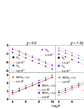
Figure 2: Scaling behaviors of some typical energies and $E2$ transition rates with respect to $N$ (log₂ by log₂) for the F(5) scheme with two $\chi$ cases.

In summary, we proposed an algebraic F(5) scheme to reveal the hidden Eu(5) DS in the critical region of the spherical–deformed SPTs. It provides thus a new perspective to understand the nuclear dynamics in the transitional region. We have shown that the Eu(5) DS can be directly translated from the geometric description of the CPS of the U(5)–O(6) transition. With the nonlinear projection, the structural evolution from the CPS of the U(5)–O(6) to that of the U(5)–SU(3) transition is realized. Our numerical analysis shows that the experimental data are reproduced well in the scheme, which indicate that the Eu(5) DS is dominant but hidden in the whole critical region of the SPT.

- (1) F. Iachello, and A. Arima, The Interacting Boson Model (Cambridge University, Cambridge, England, 1987).
- (2) F. Iachello, and R. D. Levine, Algebraic Theory of Molecules (Oxford University, Oxford, UK 1995).
- (3) H. Yépez-Martínez, J. Cseh, and P. O. Hess, Phys. Rev. C 74, 024319 (2006).
- (4) P. Cejnar, J. Jolie, and R. F. Casten, Rev. Mod. Phys. 82, 2155 (2010); P. Cejnar, and J. Jolie, Prog. Part. Nucl. Phys. 62, 210 (2009).
- (5) J. N. Ginocchio, and M. W. Kirson, Phys. Rev. Lett. 44, 1744 (1980); A. E. L. Dieperink, O. Scholten, and F. Iachello, Phys. Rev. Lett. 44, 1747 (1980); D. H. Feng, R. Gilmore, and S. R. Deans, Phys. Rev. C 23, 1254 (1981); P. Van Isacker, and J. Q. Chen, Phys. Rev. C 24, 684 (1981).
- (6) Y. Zhao, Y. Liu, L. Z. Mu, and Y. X. Liu, Int. J. Mod. Phys. E 15, 1711 (2006).
- (7) R. F. Casten, and E.A. McCutchan, J. Phys. G 34, R285 (2007); R. F. Casten, Prog. Part. Nucl. Phys. 62, 183 (2009); R. F. Casten, Nature Physics 2, 811 (2006).
- (8) D. J. Rowe, P. S. Turner, and G. Rosensteel, Phys. Rev. Lett. 93, 232502 (2004); D. J. Rowe, Phys. Rev. Lett. 93, 122502 (2004).
- (9) D. Bonatsos, E. A. McCutchan, and R. F. Casten, Phys. Rev. Lett. 104, 022502 (2010).
- (10) A. Leviatan, Phys. Rev. Lett. 98, 242502 (2007).
- (11) A. Bohr, and B. R. Mottelson, Nuclear Structure, Vol. 2, World Scientific, Singapore, 1998.
- (12) F. Iachello, Phys. Rev. Lett. 85, 3580 (2000).
- (13) M. A. Caprio, and F. Iachello, Nucl. Phys. A 781, 26 (2007).
- (14) F. Iachello, Phys. Rev. Lett. 87, 052502 (2001).
- (15) D. J. Rowe, Nucl. Phys. A 735, 372 (2004); D. J. Rowe, and P. S. Turner, Nucl. Phys. A 753, 94 (2005); D. J. Rowe, J. Phys. A 38, 10181 (2005); D. J. Rowe, T. A. Welsh, and M. A. Caprio, Phys. Rev. C 79, 054304 (2009); G. Thiamova, D. J. Rowe, and M. A. Caprio, Nucl. Phys. A 895, 20 (2012).
- (16) E. R. Marshalek, Phys. Rev. C 74, 044307 (2006).
- (17) A. Klein, C.-T. Li, and M. Vallieres, Phys. Rev. C 25, 2733 (1982).
- (18) F. Pan, and J. P. Draayer, Nucl. Phys. A 636, 156 (1998).
- (19) D. Bonatsos, E. A. McCutchan, and R. F. Casten, Phys. Rev. Lett. 101, 022501 (2008).
- (20) D. Bonatsos, E. A. McCutchan, R. F. Casten, and R. J. Casperson, Phys. Rev. Lett. 100, 142501 (2008).
- (21) D. De Frenne, Nucl. Data Sheets 110, 1745 (2009).
- (22) N. V. Zamfir, et al, Phys. Rev. C 65, 044325 (2002).
- (23) M. Kanbe and K. Kitao, Nucl. Data Sheets 94, 227 (2001).
- (24) L. Coquard, et al, Phys. Rev. C 80, 061304(R) (2009).
- (25) L. K. Peker and J. K. Tuli, Nucl. Data Sheets 82, 187 (1997).
- (26) M. R. Bhat, Nucl. Data Sheets 89, 797 (2000).
- (27) S.K. Basu, and A.A. Sonzogni, Nucl. Data Sheets 114, 435 (2013).
- (28) J. M. Arias, Phys. Rev. C 63, 034308 (2001).