Nonperturbative parton distributions and the proton spin problem

Abstract

The Lorentz contracted form of the static wave functions is used to calculate the valence parton distributions for mesons and baryons, boosting the rest frame solutions of the path integral Hamiltonian. It is argued that nonperturbative parton densities are due to excited multigluon baryon states. A simple model is proposed for these states ensuring realistic behavior of valence and sea quarks and gluon parton densities at $Q^{2}=10(GeV/c)^{2}$. Applying the same model to the proton spin problem one obtains $\Sigma_{3}=0.18$ for the same $Q^{2}$.

1 Introduction

The partonic model, which allows to express the physical amplitudes in terms of quark and gluon densities, is now widely used in many processes [1, 2, 3].

One of basic principles in this approach is the assumption, that at high momentum $P$ the wave function of a hadron can be represented as an assembly of quasi free partons – quarks and gluons – which interact perturbatively and are subject to a DGLAP evolution [3, 4, 5]. E.g. at the first step the incident object (photon) interacts with one of free quarks of the hadron, which subsequently emits gluons etc.

This idea implies, that the nonperturbative (np) interaction in the wave function of a very fast hadron can be neglected as compared to the high kinetic energy of every parton (quark or gluon). The results of this approach seem to be quite successful in many cases and the whole industry of the parton density calculations is now operating to exploit and predict experimental data [6, 7].

From the theoretical point of view this method being intuitively persuasive, still lacks rigorous foundations. It is clear, that in the rest frame the hadron wave function is governed by np interactions, such as confinement, and it is not understood how it changes with increasing velocity of the hadron.

One would like to calculate the hadron wave function in any moving frame and demonstrate the resulting transformation and transition to the pure parton picture.

Recently the possibility of this procedure was discovered in [8], where it was shown, that the Lorentz contraction condition on the wave function moving with velocity $v$, automatically brings it into a scaled partonic-like form $\psi(p_{\bot}^{(1)},...p_{\bot}^{(n)};x_{1},...x_{n})$, depending on transverse momenta $p_{\bot}^{(i)}$ and longitudinal momenta $p_{\|}^{(i)}=x_{i}P$.

The new element of this valence “partonic wave function” is the full scale np interaction, governing dependence of $\psi$ on its arguments. In particular, for the simplest $s$-wave meson wave function one obtains the form of valence component $\varphi\left(\mbox{\boldmath${\rm p}$}_{\bot},M_{0}\left(x-\frac{1}{2}\right)\right)=\varphi(\sqrt{\mbox{\boldmath${\rm p}$}^{2}_{\bot}+M^{2}_{0}(x-\frac{1}{2})^{2}})$ where $M_{0}$ is the meson rest mass and $\varphi(\mbox{\boldmath${\rm k}$})$ is the Fourier transform of the rest frame meson wave function.

It seems interesting, that the shape of the resulting quark density for this purely valence component (without Regge ladder contribution) partly resembles the known examples (at low $Q^{2}$ the maximum around $x=\frac{1}{2}$ for mesons and around 1/3 for baryons) however other features, such as admixture of antiquarks, gluons and behavior around $x=0$ and 1, are different. It is argued in the paper that the main np contribution to all parton densities at $x$ not close to 1,is coming from the high excited baryon states, and one obtains reasonable results, when the scaled partonic formalism is used for the latter.A simple model,called the multihybrid baryon model is proposed for the excited states and the results are compared to the recent data [6, 7] at $Q^{2}=10$(GeV$/c)^{2}$ and can be used as an initial step in the DGLAP evolution. Thus the use of the Lorentz contracted form of np hadron might be an interesting step in establishing of the new “nonperturbative parton model” and np quark densities. In addition, it may help to resolve the existing difficulties in the present theory, such as the proton spin problem [9], as we discuss in what follows, see also [19] for a review.

Our main result in this paper is the method of constructing the polarized and unpolarized parton densities from np wave functions (n.w.f) of any number of quarks and gluons.

In doing so we exploit the n.w.f. written in the infinite momentum frame, which has the explicit partonic scaled form. In terms of the relativistic Fock-Schwinger Hamiltonian these n.w.f. correspond to the Fock components with definite number of constituents, while the experimental data (in DIS of high energy collisions) refer to the whole Fock columns of these components, also developing in time. Therefore to get a full picture one must treat the full Fock column wave function, with all relative weights (admixtures) of different components.

We show that these admixtures of higher states to the valence component are Lorentz invariant, however strongly depend on the total energy eigenvalue of the whole Fock wave function.

E.g. the proton ground state is well represented by the valence component, while the proton high excited states may contain many additional gluons, which are seen in DIS.

We calculate the valence component of the proton pdf from the realistic proton wave function and compare it with DIS data and model (QCD sum rules) results.

At this point it is important to compare our results with the powerful method of light-cone quark models [11], see [12] for a review. In this case the Fock components also for polarized parton distributions are derived from the light-cone formalism for the wave functions. This approach has given an important tool for the analysis of experimental data, see [13], and refs. therein.

An essential new ingredient of our approach is the implementation of the np confining properties of the vacuum in the boosted instantaneous as well as in the light-cone dynamics. In the last case the corresponding Hamiltonian with confinement have been derived and studied numerically in [14, 15], demonstrating the same confining spectrum for hadrons, as in the instantaneous rest frame. The light-cone formalism is specifically convenient for the multihybrids – the string-like objects consisting of $n$ gluons “sitting” on the QCD confining string, which are possible structures behind the observed “ridges” in high-energy collisions, as discussed in [16].

In this way our approach may be a useful addition to the well developed light-cone methods in the high-energy and high-momentum QCD, introducing string-like objects in the light-cone vacuum, which are possible in the string theory context.

We start in the paper with the unpolarized parton densities for the meson and baryon cases, in the boosted instantaneous dynamics, [8], where it was shown that the np interaction is dominant in the valence Fock component, and quarks can be considered as relativistic and with suppressed spin degrees of freedom.(In addition the latter can be taken from the Pauli-Melosh basis approach of the light-front dynamics [17], see [18] for a review and references. The possible use of this formalism for the polarized pdf in our case is now under consideration.)

To include the excited states we consider the sequence of excited multigluon baryons with known form of the c.m. wave functions and find the corresponding parton form for the whole sum, which appears to be close to the recent pdf data [6, 7].

We also calculate the polarized proton pdf for the ground state proton, using the boosted factorized form of the 3q Dirac wave functions, and show that those are compatible with the spin projection criterium. Applying the same baryon multihybrid model to the spin projection criterium we find that gluons partly compensate valence quark spins leaving only about 0.2 of their spin projections.

The plan of the paper is as follows. In the next section we write the general equations for the scaled parton distributions from the nonperturbative (NP) rest frame wave functions for two and three partons. In section 3 the QCD Hamiltonian and Fock components are discussed both in the rest frame and at nigh $P$. We here calculate the proton valence pdf and compare it with known examples.

In section 4 we introduce the baryon multihybrid model and calculate pdf’s of valence and sea quarks and gluons.

In section 5 the proton spin problem is discussed for the relativistic proton wave function which ensures the correct $g_{A}/g_{V}$ ratio for the ground state proton. The contribution of excited states is considered in the framework of the baryon multihybrid model and the resulting value of $\Sigma_{3}$ is calculated.

The last section is devoted to the Summary of the results and prospectives.

2 Parton densities from the Lorentz contracted wave functions

The multiparton wave function normalized in a standard way [2]

$$E(P)\int\prod^{N}_{i=1}\frac{d^{3}p_{i}}{\varepsilon_{i}}\delta^{(3)}\left(\mbox{\boldmath${\rm P}$}-\sum^{n}_{k=1}\mbox{\boldmath${\rm p}$}_{k}\right)|\psi(p_{1},...p_{N})|^{2}=1,\varepsilon_{i}=\sqrt{\mbox{\boldmath${\rm p}$}^{2}_{i}+m^{2}_{i}}$$ (1)

in the limit of large $P$ is written as

$$\int\prod d^{2}p_{\bot}^{(i)}\frac{dx_{i}}{x_{i}}\delta^{(2)}(\sum^{N}_{i=1}\mbox{\boldmath${\rm p}$}_{\bot}^{i})\delta(1-\sum^{N}_{i=1}x_{i})|\psi(p_{\bot}^{(i)},x_{i})|^{2}=1.$$ (2)

It can be connected to the Lorentz contracted rest frame wave function $\tilde{\varphi}_{0}(k_{\bot}^{(1)},k_{\bot}^{(2)},...;k_{\|}^{(1)}\sqrt{1-v^{2}},...)$ which is normalized in the rest frame as

$$M_{0}\int|\tilde{\varphi}(\mbox{\boldmath${\rm k}$}^{(1)}\mbox{\boldmath${\rm k}$}^{(2)}...)|^{2}\frac{d^{3}\mbox{\boldmath${\rm k}$}^{(1)}}{(2\pi)^{3}}...\frac{d^{3}\mbox{\boldmath${\rm k}$}^{(N)}}{(2\pi)^{3}}(2\pi)^{3}\delta^{(2)}(\sum\mbox{\boldmath${\rm k}$}_{\bot}^{(i)})\delta(1-\sum x_{i})=1,$$ (3)

where $k^{(i)}_{\|}=M_{0}(x_{i}-\nu_{i})$.

The parton distribution in the hadron $h$ is $D^{q}_{h}(x,k_{\bot})$, which is defined as

$$D^{q}_{h}(x,k_{\bot})=\sum_{n}\prod_{r}\frac{d^{3}k_{r}}{\varepsilon_{r}}E_{h}^{2}\delta^{(3)}(P-\sum k_{r})|\psi_{h}^{(n)}(k_{r},\lambda_{r})|^{2}\sum_{r(j)}\delta^{(3)}(k-k_{j}))$$ (4)

$D^{q}_{h}(x,k_{\bot})$ satisfies the following conditions [2]

$$\int d^{2}k_{\bot}dxD_{h}^{q_{j}}(x,k_{\bot})=N_{h}^{j},$$ (5)

where $N^{j}_{h}$ is the number of partons of the type $j$ in the hadron $h$, and normalization condition

$$\sum_{j}\int d^{2}k_{\bot}dxxD_{h}^{q_{j}}(x,k_{\bot})=1.$$ (6)

One can also define the parton density

$$D^{q}_{h}(x)=\int d^{2}k_{\bot}D^{q}_{h}(x,k_{\bot})$$ (7)

In terms of the meson rest frame wave function one can write, taking into account, that it depends on the relative momentum ${\rm k}$ in the rest frame

$$D^{q}_{M}(x)=\frac{M^{2}_{0}}{(2\pi)^{3}}\left|\tilde{\varphi}_{0}^{(2)}\left(k_{\bot},M_{0}\left(x-\frac{1}{2}\right)\right)\right|^{2},$$ (8)

where the meson wave function is normalized as

$$\frac{M^{2}_{0}}{(2\pi)^{3}}\int\left|\tilde{\varphi}_{0}^{(2)}\left(k_{\bot},M_{0}\left(x-\frac{1}{2}\right)\right)\right|^{2}d^{2}k_{\bot}dx=$$

$$=\frac{M_{0}}{(2\pi)^{3}}\int\left|\tilde{\varphi}_{0}^{(2)}\left(k_{\bot},k_{\|}\right)\right|^{2}d^{3}k=1$$ (9)

From the condition $\int\left(x-\frac{1}{2}\right)|\tilde{\varphi}^{(2)}_{0}|^{2}d^{2}k_{\bot}dx=0$ and normalization condition (9) one obtains both relations (5) and (6).

For the $3q$ valence wave function of the baryon one can write, e.g. for the $u$ quark distribution in the proton (ignoring spin degrees of freedom, see section 4)

$$u(x,k_{\bot})=\int\delta^{(2)}\left(\sum^{3}_{i=1}k_{\bot i}\right)\prod^{3}_{i=1}d^{2}k_{\bot i}dx_{1}dx_{2}dx_{3}\delta\left(1-\sum x_{i}\right)\times$$

$$\times\frac{M_{0}^{3}}{(2\pi)^{3}}|\tilde{\varphi}_{0}^{(3)}|^{2}[(\delta^{(2)}(k_{\bot}-k_{\bot 1})\delta(x-x_{1})+(1\leftrightarrow 2))]$$ (10)

where $\tilde{\varphi}^{(3)}_{0}$ is $\tilde{\varphi}^{(3)}_{0}\left(k_{\bot 1},...k_{\|1}^{(0)},...\right).$

The normalization of the $\tilde{\varphi}_{0}^{(3)}$ is

$$\frac{M^{3}_{0}}{(2\pi)^{6}}\int\prod^{3}_{i=1}d^{2}p^{(i)}dx_{i}\delta^{(2)}\left(\sum^{3}_{i=1}p_{\bot}^{(i)}\right)\delta\left(1-\sum^{3}_{i=1}x_{i}\right)\left|\tilde{\varphi}_{0}^{(3)}(p_{\bot,...,}x_{i}\right|^{2}=1.$$ (11)

In a similar way one defines the $d$ quark distribution, in which case one will have one product of $\delta$ functions instead of the sum of two products in the square brackets in (10).

For the 3-particle wave function and Hamiltonian it is convenient to introduce the total momentum ${\rm P}$ and two relative momenta $\mbox{\boldmath${\rm\pi}$},\mbox{\boldmath${\rm q}$}$ defined as follows [20, 21] (we assume for simplicity particles 1 and 2 to be identical)

$$\mbox{\boldmath${\rm\eta}$}=\frac{\mbox{\boldmath${\rm z}$}^{(1)}-\mbox{\boldmath${\rm z}$}^{(2)}}{\sqrt{2}},~{}~{}\mbox{\boldmath${\rm\xi}$}=\sqrt{\frac{\omega_{3}}{2\omega}}(\mbox{\boldmath${\rm z}$}^{(1)}+\mbox{\boldmath${\rm z}$}^{(2)}-2\mbox{\boldmath${\rm z}$}^{(3)})$$

$$\mbox{\boldmath${\rm R}$}=\frac{1}{\Omega}\sum^{3}_{i=1}\omega_{1}\mbox{\boldmath${\rm z}$}^{(i)},~{}~{}\Omega=\sum^{3}_{i=1}\omega_{i},~{}~{}\omega_{1}=\omega_{2}=\omega$$ (12)

$$\mbox{\boldmath${\rm P}$}=\frac{\partial}{i\partial\mbox{\boldmath${\rm R}$}},~{}~{}\mbox{\boldmath${\rm q}$}=\frac{\partial}{i\partial\mbox{\boldmath${\rm\xi}$}},~{}~{}\mbox{\boldmath${\rm\pi}$}=\frac{\partial}{i\partial\mbox{\boldmath${\rm\eta}$}}$$

$$H=\frac{\mbox{\boldmath${\rm P}$}^{2}}{2\Omega}+\frac{\mbox{\boldmath${\rm q}$}^{2}+\mbox{\boldmath${\rm\pi}$}^{2}}{2\omega}+\sum^{3}_{i=1}\frac{m^{2}_{i}+\omega^{2}_{i}}{2\omega_{i}}+V(\mbox{\boldmath${\rm\eta}$},\mbox{\boldmath${\rm\xi}$}).$$ (13)

In terms of individual momenta $\mbox{\boldmath${\rm p}$}^{(i)}=\frac{1\partial}{i\partial\mbox{\boldmath${\rm z}$}^{(i)}}$ one has the following connection

$$\mbox{\boldmath${\rm p}$}^{(1)}=\frac{\omega}{\Omega}\mbox{\boldmath${\rm P}$}+\sqrt{\frac{\omega_{3}}{2\Omega}}\mbox{\boldmath${\rm q}$}-\frac{\mbox{\boldmath${\rm\pi}$}}{\sqrt{2}}$$

$$\mbox{\boldmath${\rm p}$}^{(2)}=\frac{\omega}{\Omega}\mbox{\boldmath${\rm P}$}+\sqrt{\frac{\omega_{3}}{2\Omega}}\mbox{\boldmath${\rm q}$}+\frac{\mbox{\boldmath${\rm\pi}$}}{\sqrt{2}}$$

$$\mbox{\boldmath${\rm p}$}^{(3)}=\frac{\omega_{3}}{\Omega}\mbox{\boldmath${\rm P}$}-\sqrt{\frac{2\omega_{3}}{\Omega}}\mbox{\boldmath${\rm q}$}$$ (14)

Note, that $\omega_{i}$ are found from the stationary point analysis of $M_{n}(\omega_{1},\omega_{2},\omega_{3})$ the eigenvalue of $H$, namely from the relations

$$\left.\frac{\partial M_{n}(\{\omega_{i}\})}{\partial\omega_{k}}\right|_{\omega_{k}=\omega_{k}^{(0)}}=0.$$ (15)

Since $\tilde{\varphi}_{0}^{(3)}$ is the Fourier transform of the rest frame wave function, we shall use finally the values of $\omega_{i}^{(0)}$ obtained in the rest frame.

Using (14) one can write in (11)

$$\delta^{(2)}(\sum^{3}_{i=1}\mbox{\boldmath${\rm p}$}_{\bot}^{(i)})\prod d^{2}\mbox{\boldmath${\rm p}$}_{\bot}^{(i)}=\frac{\omega_{3}}{\Omega}d^{2}\mbox{\boldmath${\rm P}$}_{\bot}d^{2}q_{\bot}d^{2}\mbox{\boldmath${\rm\pi}$}_{\bot}d^{2}\mbox{\boldmath${\rm\pi}$}_{\bot}\delta(\mbox{\boldmath${\rm P}$}_{\bot})=\frac{\omega_{3}}{\Omega}d^{2}\mbox{\boldmath${\rm q}$}_{\bot}d^{2}\mbox{\boldmath${\rm\pi}$}_{\bot}.$$ (16)

To find the arguments $p_{\|i}^{(0)}(x_{i})$ in (10), (11), which are the longitudinal components of parton momenta in the rest frame, we use the Lorentz connection of these to the momenta in the moving frame

$$p_{\|i}=\frac{p_{\|i}^{(0)}+v\bar{\omega}^{(0)}_{i}}{\sqrt{1-v^{2}}}=Px_{i},$$ (17)

which yields

$$p_{\|i}^{(0)}=\left(x_{i}-\frac{\bar{\omega}_{i}^{(0)}}{M_{0}}\right)M_{0}.$$ (18)

In what follows we shall accept for simplicity the relation for massless quark $\bar{\omega}_{i}^{(0)}\equiv\bar{\omega}^{(0)},~{}~{}i=1,2,3$ and the relation for the total mass in the case of free quarks, which holds approximately true in the interacting case $M_{0}=\sum^{3}_{i=1}\bar{\omega}_{i}^{(0)}=3\bar{\omega}^{(0)},$ hence $p_{i\|}^{(0)}=\left(x_{i}-\frac{1}{3}\right)M_{0}$. For the relative momenta one obtains

$$q_{\|}^{(0)}=\frac{M_{0}}{\sqrt{6}}(x_{1}+x_{2}-2x_{3}),~{}~{}\pi_{\|}^{(0)}=\frac{M_{0}(x_{2}-x_{1})}{\sqrt{2}}.$$ (19)

One can rewrite the normalization condition (11) as

$$1=\frac{M^{3}_{0}}{(2\pi)^{6}}\cdot\frac{1}{3}\int d^{2}\mbox{\boldmath${\rm q}$}_{\bot}d^{2}\mbox{\boldmath${\rm\pi}$}_{\bot}dx_{1}dx_{2}dx_{3}\delta\left(1-\sum^{3}_{i=1}x_{i}\right)\left|\tilde{\varphi}_{0}^{(3)}(\mbox{\boldmath${\rm q}$}_{\bot},\mbox{\boldmath${\rm\pi}$}_{\bot},q_{\|}^{(0)},\pi_{\|}^{(0)}\right|^{2}$$ (20)

and Eq. (10) acquires the form

$$u(x,k_{\bot})=\frac{4M^{3}_{0}}{(2\pi)^{3}}\int d^{2}\mbox{\boldmath${\rm\pi}$}_{\bot}\int^{1}_{0}$$

$$dx_{2}\left|\tilde{\varphi}^{(3)}_{0}\left(\sqrt{3}\mbox{\boldmath${\rm\pi}$}_{\bot}+\sqrt{6}\mbox{\boldmath${\rm k}$}_{\bot};\mbox{\boldmath${\rm\pi}$}_{\bot};\sqrt{\frac{3}{2}}M_{0}\left(x+x_{2}-\frac{2}{3}\right);\right.\left.\left(\frac{M_{0}(x_{2}-x)}{\sqrt{2}}\right)\right)\right|^{2}.$$ (21)

It is known, however, that the nucleon wave function can be expanded in the series of hyperspherical harmonics [21], and the leading term accounts for $\sim 90\%$ of the normalization condition. This means, that $\tilde{\varphi}_{0}^{(3)}$ can be considered as the function of

$$\mbox{\boldmath${\rm Q}$}^{2}=\mbox{\boldmath${\rm\pi}$}^{2}+\mbox{\boldmath${\rm q}$}^{2}=\mbox{\boldmath${\rm\pi}$}^{2}_{\bot}+\mbox{\boldmath${\rm q}$}^{2}_{\bot}+(\pi_{\|}^{(0)})^{2}+(q_{\|}^{(0)})^{2}=\mbox{\boldmath${\rm\pi}$}^{2}_{\bot}+\mbox{\boldmath${\rm q}$}^{2}_{\bot}+\frac{M_{0}^{2}}{3}\sum_{i>j}(x_{i}-x_{j})^{2}.$$ (22)

As a result the argument of $\tilde{\varphi}_{0}^{(3)}$ in (21) can be written as

$$\tilde{\varphi}^{(3)}_{0}(\mbox{\boldmath${\rm Q}$}^{2})\to\tilde{\varphi}^{(3)}_{0}(4\mbox{\boldmath${\rm\pi}$}^{2}_{\bot}+6\mbox{\boldmath${\rm k}$}^{2}_{\bot}+6\sqrt{2}\mbox{\boldmath${\rm\pi}$}_{\bot}\mbox{\boldmath${\rm k}$}_{\bot}+\frac{2M_{0}^{2}}{3}f(x,x_{2}))$$ (23)

where

$$f(x,x_{2})=1+3x^{2}+3x^{2}_{2}+3xx_{2}-3x-3x_{2}=3\left(\left(x_{2}-\frac{1-x}{2}\right)^{2}+c(x)\right),$$ (24)

$$~{}~{}c(x)=\frac{9x^{2}-6x+1}{12}.$$

It is conceivable, that after the integration over $d^{2}\mbox{\boldmath${\rm\pi}$}_{\bot}$ and $dx_{2}$ the result will depend mostly on $c(x)$, which has the minimum at $x=\frac{1}{3}$ and hence $u(x,k_{\bot})$ as a function of $x$ would have a maximum around that point.

This result is close to that obtained for the valence quark density in [22] and has a form similar to the DIS data [7], [23] at low $Q^{2}$. In Fig. 1 we compare our results with those of [22]. We shall argue however, that the DIS data refer to the high excited baryon state, and hence could differ from the ground state proton case. In section 4 we provide a simple model of excited states which yields reasonable results at $Q^{2}=10$ (GeV/c)² and can be used for the DGLAP evolution.

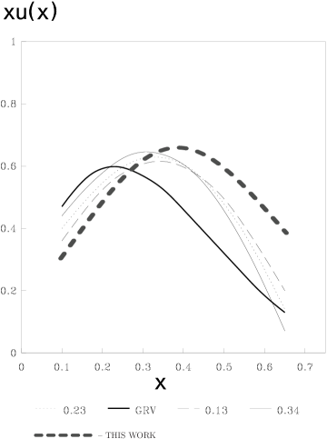
Figure 1: The valence parton distribution in proton (thick dashed line) in comparison with the results of [22] for fixed values of quark condensate, and results of the second reference [7], – thick solid line (GRV).

Note, that our hyperspherical approximation for the proton wave function used in Fig.1, thick dashed line, is applicable around $x=1/3$ and not suitable for the region of small 1-x, where quark carries all proton momentum and one expects the behavior $u(x)\sim(1-x)^{2}$ in the free parton case.

3 The QCD Hamiltonian and Fock components

We assume in this section that one can construct a QCD Hamiltonian, which provides eigenvalues and eigenfunction for all Fock components, e.g. in case of a baryon state, the pure valence state $(qqq)$, also with any number of additional gluons $(qqqg),(qqqgg),...,$ which are actually hybrid states, and with additional $q\bar{q}$ pairs:$(qqq(q\bar{q}))$ etc.

One example of such Hamiltonian is provided by the path integral Hamiltonian derived in the framework of the Fock-Feynman-Schwinger Representation (FFSR) [24], and developed further in [25, 26]. It was used for mesons [27], baryons [21, 28], hybrids [29] and glueballs [30]. yielding in all cases spectra in good agreement with experimental and lattice data.

The full Fock matrix Hamiltonian in this case consists of the diagonal elements $H_{nn}^{(0)}$ for each $n$-th Fock component and of the nondiaginal elements $H_{nk}$, $n\neq k$, which are actually elements of the interaction vertices $V_{nk}$. In what follows we are using the line of reasoning from [31, 32] and start with the center of mass frame, $\mbox{\boldmath${\rm P}$}=0$. Note, that we have the instantaneous dynamics, so that all operators $\hat{H}=\hat{H}^{(0)}+\hat{V}$ do not depend on time, and $\hat{V}$ acts at the instantaneous moment of creation or destruction of an additional particle.

In Fig.2 it is shown, how subsequent Fock components appear in the meson Green’s function, where additional gluons and a $q\bar{q}$ pair are created by the interaction $V_{nk}$.

Figure 2: The meson Green’s function, containing the Fock components: $q\bar{q}$ (sector I), $q\bar{q}g$ (sector II and sector III), $q\bar{q}gg$ (sector IV) and $q\bar{q}q\bar{q}$ (sector V). Note, that all surface between external solid lines is filled in by the string world sheet, except for the narrow gap between $q\bar{q}$ lines in sector V

One can simplify, as in [31], the structure of $\hat{H}$, and taking the limit of large $N_{c}$, so that an additional $q\bar{q}$ pair “costs” a factor of $1/N_{c}$, while an additional glueball gives $1/N_{c}^{2}$, so that all Fock components reduce to the pure valence states and its hybrid excitations.

The basic matrix equation is simply

$$\hat{H}\Psi_{N}=(\hat{H}^{(0)}+\hat{V})\Psi_{N}=E_{N}\Psi_{N},$$ (25)

and the Fock column $\Psi_{N}\{P,\xi,n\}$ has quantum numbers $N=0,1,2$… of the ground and excited states, $n$ refers to the Fock column number, and $\xi$ denotes additional internal numbers for a given type of excitation. In the diagonal approximation $\Psi_{N}\to\Psi_{N\{P,\xi,n\}}$ with $n=n^{(0)}$. Note, that for $N_{c}\to\infty$ and baryon number $B=1$ one has only discrete spectrum of a valence and hybrid states. In this case the eigenvalues for $\mbox{\boldmath${\rm P}$}\neq 0$ are simply

$$E_{N}^{(0)}=E_{n}^{(0)}(P)=\sqrt{\mbox{\boldmath${\rm P}$}^{2}+M^{2}_{n\{k\}}}.$$ (26)

and the eigenfunctions are $\psi_{n}(P,\xi,k)\equiv\psi_{n,k}$, where $\xi,k$ comprise radial and angular $(k)$, as well as additional $(\xi)$ quantum numbers. The set $\psi_{n\{k\}}$ can be used to expand the total wave function $\Psi_{N}$, (discrete spectrum at $N_{c}\to\infty$)

$$\Psi_{N}=\sum_{m\{k\}}c^{N}_{m\{k\}}\psi_{m\{k\}},~{}~{}\int\Psi^{+}_{N}\Psi_{M}d\Gamma=\sum_{m\{k\}}c^{N}_{m\{k\}}c^{M}_{m\{k\}}=\delta_{NM}.$$ (27)

As in [31, 32], we use the orthonormality condition

$$\int\psi^{+}_{m\{k\}}\psi_{n\{p\}}d\Gamma=\delta_{mn}\delta_{\{k\}\{p\}}$$ (28)

to find the equation for $c$ and $\Psi$

$$c^{N}_{n\{p\}}(E_{N}-E^{(0)}_{n\{p\}})=\sum_{m\{k\}}c^{N}_{m\{k\}}V_{n\{p\},m\{k\}}$$ (29)

with

$$V_{n\{p\},m\{k\}}=\int\psi^{+}_{n\{p\}}\hat{V}\psi_{m\{k\}}d\Gamma.$$ (30)

to the first order in $V$ one has

$$C^{N(1)}_{n\{p\}}=\frac{V_{n\{p\},\nu\{\kappa\}}}{E^{(0)}_{\nu\{\kappa\}}-E^{(0)}_{n\{p\}}}$$ (31)

and for the high Fock component with $l$ gluons in addition to the valence quarks one has in the lowest approximation

$$C^{N(\nu\{\kappa\})}_{\nu+l,\{k\}}=\sum_{\{k_{1}\}...\{k_{l}\}}\frac{V_{\nu+l\{k\},\nu+l-1\{k_{1}\}}}{E^{(0)}_{\nu\{\kappa\}}-E^{(0)}_{\nu+l\{k\}}}\frac{V_{\nu+l-1\{k_{1}\},\nu+l-2\{k_{2}\}}}{E^{(0)}_{\nu\{\kappa\}}-E^{(0)}_{\nu+l-1\{k_{1}\}}}...$$

$$\frac{V_{\nu+1\{k_{l}\},\nu\{\kappa\}}}{E^{(0)}_{\nu\{\kappa\}}-E^{(0)}_{\nu+1\{k_{l}\}}}+O(V^{l+2}).$$ (32)

Using (27), (28), one can obtain the equality

$$\sum_{n\{k\}}\left|C^{N}_{n\{k\}}\right|^{2}=1,$$ (33)

and each state $N$ can be characterized by the sequence

$$\{|C^{N}_{0}|^{2},|C_{1\{k\}}^{N}|^{2},...\}\equiv\{C^{N}\}.$$

Note, that $\hat{V}$ is $O(g)$, and hence in the limit $g\to 0$ one has the unmixed states $\{1,0,0,...\},\{0,1,0,...\}$ etc., while the inclusion of $\hat{V}$ starts the “evolution” of the basic state along the chain of neighboring states. This can be done in principle in accordance with the DGLAP evolution equation, to be written in terms of parton distribution functions (pdf), i.e. in terms of $|\psi_{n\{k\}}|^{2}$ integrated over all pairs $p_{\bot}^{(i)}$ and $x_{i}$, except one, $\mbox{\boldmath${\rm p}$}_{\bot}^{(i)}\equiv\mbox{\boldmath${\rm k}$}_{\bot},x_{1}\equiv x$.

Thus the nonperturbative $N_{c}\to\infty$ limit of the evolution is given by (29), (31). At this point it is important to stress, that sequences $\{C^{N}\}$ can be completely different for the baryon ground state with $E_{0}=m_{p}$, and the highly excited baryon state with a large c.m. energy $E_{N}$. In our case $(N_{c}=\infty)$ this refers to the discrete spectrum, while allowing for the $q\bar{q}$ pairs one has a continuous spectrum. Indeed, as was estimated in [32, 33] for the meson-hybrid mixing coefficient $V_{Mh}\sim g\cdot 0.08$ GeV and

$$C_{Mh}=\frac{V_{Mh}}{E^{(0)}_{M}-E^{(0)}_{h}}=\frac{V_{Mh}}{\Delta M_{Mh}},~{}~{}\Delta M_{Mh}\sim O(1~{}{\rm GeV})$$ (34)

which gives the hybrid admixture $|C_{Mh}|^{2}\approx O(1\%)$. As shown in [31, 32] the addition of one gluon to the hybrid state “costs” around 1 GeV, hence multigluon states contribute very little to the ground state wave function. For the high excited states the denominator in (34) can be much smaller and the total number of mixing states grows, so that the gluon admixture should grow substantially.

This is exactly what happens in DIS. Indeed, the c.m. energy of the baryon state, with initial momentum $p$, exited by the incident virtual $\gamma$ or $W,Z$ with momentum $q$, is very high in the Bjorken limit.

$$s=m^{2}_{B}+2\nu(1-x),~{}~{}x=Q^{2}/2\nu,~{}~{}s-m^{2}_{B}=2\nu(1-x)\gg m_{B}^{2}.$$

In Fig. 3 we show schematically how the excited baryon state emerges in DIS.

Figure 3: The excited baryon state created in DIS has the excitation energy in the rest frame $E_{CM}=\sqrt{M^{2}_{B}+\frac{Q^{2}(1-x)}{x}}$, which is much larger than $M_{B}$ and the boost momentum $Q$ for small $x$

.

It is actually the baryon state with the c.m. energy $E_{cm}=\sqrt{s}$, which is tested in DIS and the resulting pdf refer to this $E_{cm}$, which is close to $m^{2}_{B}$ only at the end point $x=1$. Therefore one should expect, that at growing $s=m^{2}_{B}+\frac{Q^{2}}{x}(1-x)$ the admixture of gluons should grow fast, since the coefficients (32) increase with energy, or equivalently, DGLAP evolution at high $Q^{2}$ produce a large gluon component, see e.g. [6, 23]. We stress again., that this fact refers not to the ground state described above. For the ground state baryon (or meson) the sequence $\{C^{N}\}$ is fast decreasing and is given by the rest frame wave functions, described in the previous section.

One of the consequences of this discussion is the possible resolution of the proton spin problem in the next section (see [9] for discussion and references). Indeed, insertion in the proton wave function the polarized parton distributions, obtained from the highly excited baryon states, results in the high admixture of the antiquark and gluon components (which are suppressed in the genuine proton wave function). As a result the contribution of the valence quarks is very small, and one faces the strange picture of the almost quarkless proton. If instead one uses the pdf of the multigluon baryon, described in the next section, this discrepancy disappears, as we show in the section 5.

One should stress in addition, that the virtual photon in DIS is able to transfer any amount of the angular momentum (similarly to the process of the electroexcitation of nuclei), so that the excited baryon can have any half integer spin, suppressing in this way the contribution of the $s=1/2$.

We now turn to the boosted form of the hadron wave function. We assume, as in [8], that the boost acts on the spacial wave function $\Psi_{N}$ as the Lorentz contraction, while the interaction term $\hat{V}$ behaves as $L\hat{V}=CV,~{}~{}C_{0}=\sqrt{1-v^{2}}.$

This becomes clear from (25), if one writes the Hamiltonian in (25) in the off-shell form as in (13)

$$\hat{H}^{(0)}=\frac{\mbox{\boldmath${\rm P}$}^{2}+\Omega^{2}}{2\Omega}+\sum^{N}_{i=1}\frac{m^{2}_{i}+\omega^{2}_{i}+\mbox{\boldmath${\rm p}$}^{2}_{i}}{2\omega_{i}}+\frac{C(V_{0}+\Delta V)\bar{M}}{2\Omega},$$ (35)

where we have splitted the interaction $\hat{V}=V_{0}+\Delta V$ into a diagonal and nondiagonal parts in the number $n$ of constituents.

As a result

$$E_{n}^{(0)}=\sqrt{\mbox{\boldmath${\rm P}$}^{2}+(M_{n}^{(0)})^{2}}\simeq P+\frac{(M_{n}^{(0)})^{2}}{2P}+...$$

and

$$C_{n\{P\}|^{N}\{1\}}=\frac{CV^{(0)}_{n,n\pm 1}}{E^{(0)}_{n\pm 1}-E_{n}^{(0)}}\simeq\frac{C_{0}PV_{n,n\pm 1}^{(0)}}{(M^{(0)}_{n\pm 1})^{2}-(M_{n}^{(0)})^{2}}\simeq\frac{M_{n}^{(0)}V_{n,n+1}^{(0)}}{(M^{(0)}_{n\pm 1})^{2}-(M_{n}^{(0)})^{2}}.$$ (36)

Hence the set $\{C^{N}\}$ (34) is boost invariant and the nucleon mixing contents does not change, when going from the rest frame to the infinite momentum frame. The same can be said about all excited baryon states, which are measured using 4-point amplitudes, as it is done in DIS, and the high excited energy states (about tens of GeV on average) are very different from the ground state nucleon both in the c.m. and infinite momentum frames. In the DIS partonic set $\{C^{N}\}$ one has much higher admixture of antiquark and gluon (hybrid) components, as compared to the ground state nucleon partonic set. This possibly explains the long standing proton spin puzzle [9], where the use of the polarized DIS data yields high antiquark admixture, cancelling the valence quark contribution, and high gluon contribution.

At this point it is essential to note, that the very idea, that the high excited hadron can be represented by an assembly of almost free partons seems to be reasonable, but the idea, that the fast moving ground state hadron can be represented by the same set of free partons from our point of view has no foundations.

It is important, that in DIS we talk about the high-excited baryon Green’s function and parton distributions, which is especially evident, when one considers the Regge exchange contribution to the parton densities.

In some cases, as in DIS, quantum numbers of this high-excited object can be the same, as for a nucleon, but we stress, that the ground state nucleon has little to do with this object quark densities, while it is likely, that the high excited hadron can simulate the observed quark distribution. It is even likely, that at very high excitation the nonperturbative contributions can be treated as the initial state to the evolution of partons subject to the DGLAP or BFKL procedure, see e.g. [34].

4 Nonperturbative model of DIS parton distributions in proton

The purpose of this section is to provide a simple model of the np DIS process,which can demonstrate a large gluon (and sea quark) component at small $x$, found in the data [6, 7], as compared to the valence component. To this end we consider the region of $x$ not close to 1 and $Q^{2}$ around 10 (GeV/c)² and we expect that the main part of all products in DIS is the result of the set of high excited baryonic states, which in the limit $N_{c}\to\infty$ one can associate with the multihybrid states [16].

For the multihybrid state, which is the basic component in the large $N_{c}$ limit, the gluons, depicted as broken lines in Fig. 3, are connected by the QCD string,and the corresponding structure is actually the excited gluon string, where excitations have the particle-like form,as it is known in hybrids [29, 31, 32].

We shall use the parton distribution function (pdf) $D^{i}_{N}(x)$ as in (4), and we shall try the factorization ansatz for the wave function of the N- multihybrid, consisting of 3 quarks and N gluons

$$|\Psi^{N}_{B}(k_{\bot i},k_{\|i})|^{2}=\prod^{N+3}_{i=1}|\varphi_{i}(k_{\bot i},k_{\|i})|^{2},$$ (37)

where $\varphi_{i}$ can be written as $\varphi_{i}((k_{\bot}i)^{2},(k_{\|}i)^{2})$ and according to [8] the parton form is obtained as follows

$$\varphi_{i}(k_{\bot},k_{\|})=\varphi_{i}((k_{\bot})^{2}+M_{N}^{2}(x_{i}-\nu_{i})^{2}).$$ (38)

The Hamiltonian for the 3q multihybrid state, consisting of 3 quarks and N gluons, ”sitting ” on the strings connecting quarks to the string junction, can be written in full analogy to the case of the $q\bar{q}$ multihybrid state studied in [29, 31, 32], where quarks and gluons entered additively. Therefore one can write the resulting total energy as

$$M_{N}=3\omega+Nm,3\omega=M_{p},$$ (39)

where $\omega$ and $m$ are c.m. energies of the quark and gluon respectively. In the wave function (39)the term $\nu_{i}$ according to [8] can be written as

$$\nu_{q}=\omega/M_{N},~{}~{}\nu_{g}=m/M_{N}.$$ (40)

In the large N limit one can write $D_{N}^{i}(x)$ as follows

$$D_{N}^{i}(x)=f_{i}^{(N)}(M_{N}|x-\nu_{i}|),~{}i=q,g$$ (41)

where $f_{i}(y)$ is subject to the normalization condition

$$\int^{1}_{0}f_{i}(x)dx=1.$$

In the particular case of the Gaussian wave function, which was shown in [16, 32] to be a good approximation for the multihybrid wave function, one has

$$f_{i}^{(N)}(M_{N}|x-\nu|)=\xi_{i}^{(N)}\frac{M_{N}}{\kappa}\exp(-\frac{M_{N}^{2}}{\kappa^{2}}(x-\nu_{i})^{2}),$$ (42)

and $\xi_{i}$ is defined by the normalization condition of $f_{i}$.

We are now in a position to construct pdf for quarks and gluons, which can serve as a nonperturbative input at some $Q^{2}$ and being evolved by the DGLAP mechanism. One of not still understood features of the standard theory is the pdf behavior at very small $x<10^{-3}$, where $xg(x)$ is diverging (seemingly as $x^{-0.5}$, while $xu(x)$ is behaving approximately as $x^{0.5}$ [6, 7].

In what follows we shall be mostly interested in this region of $x$, leaving the region near $x=1$ for the lack of space, and we shall show, that our model can explain this dependence at $Q^{2}=10$(GeV/c)², while gluon evolution and quark pair production can explain the behavior at larger $Q^{2}$. To this end we assume that the main step in the DIS process is the creation of the multihybrid baryon sequence of states with coefficients $C_{N}$, satisfying the orthonormality condition (33)

$$|C_{0}|^{2}+\sum^{\infty}_{N=1}|C_{N}|^{2}=1.$$ (43)

Note,that $|C_{0}|^{2}$ gives the prbability of the pure baryon state (without gluons, but with radial and orbital excitations), which we combine into one baryon state, and similarly for $|C_{N}|^{2}$ which include possible excitations. We shall have in mind the limit of large $N_{c}$, which allows for gluon multiplication, but forbids in the lowest order the $q\bar{q}$ creation by gluons.

As a result one can write

$$g(x)=\sum^{\infty}_{N=1}Nf_{g}^{(N)}(x),~{}~{}u_{v}(x)=2\sum^{\infty}_{N+1}f_{q}^{(N)}(x)+2f_{q}^{(0)}(x).$$ (44)

Inserting $f_{i}^{(N)}$ from (43) one obtains

$$u_{v}(x)=u_{0}(x)+u_{g}(x),$$ (45)

where $u_{0}(x)$ and $u_{g}(x)$ are

$$u_{0}(x)=2|C_{0}|^{2}M_{p}\frac{\xi_{q}^{(0)}}{\kappa}\exp{(-\frac{M_{p}^{2}}{\kappa^{2}}(x-1/3)^{2})}$$ (46)

$$u_{g}(x)=2\sum^{\infty}_{N=1}|C_{N}|^{2}\xi_{q}^{(N)}(M_{p}+mN)\exp{(-\frac{M_{N}^{2}}{\kappa^{2}}(x-\nu_{q})^{2})},$$ (47)

$$g(x)=\sum^{\infty}_{N=1}|C_{N}|^{2}|\xi_{g}^{(N)}N\frac{M_{p}+Nm}{\kappa}\exp\left\{\left(-\frac{M_{N}^{2}}{\kappa^{2}}(x-\nu_{g})^{2}\right)\right\}.$$ (48)

Here $\xi_{q,g}$ are defined by normalization

$$\xi_{q}^{-1}=\int^{\frac{M_{N}}{\kappa}}_{0}dy\exp{(-(y-\omega/\kappa)^{2})}$$ (49)

$$\xi_{g}^{-1}=\int^{\frac{M_{N}}{\kappa}}_{0}dy\exp{(-(y-m/\kappa)^{2})}.$$ (50)

At this point, having in mind that the effective region of $N$ in the sums over $N$ is $N\gg 1$, it is useful to replace the sums by the integrals over $N$ and change variables as follows

$$y=\frac{Nmx}{\kappa},~{}~{}N=\frac{y\kappa}{mx}.$$ (51)

To obtain the resulting difference in the behavior of $u_{v}(x),g(x)$ we assume the ansatz

$$|C_{N}|^{2}=N^{-3/2}|\bar{c}|^{2},~{}~{}N\gg 1.$$ (52)

As a result we are left with the parameters $m,\kappa,|c_{0}|^{2},|\bar{c}|^{2}$, the latter satisfying the condition

$$|c_{0}|^{2}+|\bar{c}|^{2}\zeta(3/2)=1,\zeta(3/2)=2.62,$$ (53)

and $u_{v}(x),g(x)$ assume the form

$$u_{0}(x)=2M_{p}|c_{0}|^{2}\xi_{q}^{(0)}\kappa^{-1}\exp{(-\frac{M_{p}^{2}}{\kappa^{2}}(x-1/3)^{2})},$$ (54)

$$u_{g}(x)=2|\bar{c}|^{2}\xi_{q}(\sqrt{\frac{m}{\kappa x}}I_{q}(-1/2)+\frac{M_{p}}{\kappa}\sqrt{\frac{mx}{\kappa}}I_{q}(-3/2)),$$ (55)

$$g(x)=|\bar{c}|^{2}\xi_{g}(\sqrt{\frac{M_{p}^{2}}{\kappa mx}}I_{g}(-1/2)+\sqrt{\frac{\kappa}{m}}x^{-3/2}I_{g}(1/2)),$$ (56)

where notation is used

$$I_{q}(n)=\int^{\infty}_{mx/\kappa}dyy^{n}\exp{(-(\frac{M_{p}x-\omega}{\kappa}+y)^{2})},$$ (57)

$$I_{g}(n)=\int^{\infty}_{mx/\kappa}dyy^{n}\exp{(-(\frac{M_{p}x-m}{\kappa}+y)^{2})},$$ (58)

and we have taken the asymptotic values

$$\xi_{q}=(1.63)^{-1},\xi_{g}=(1.77)^{-1},\xi_{q}^{(0)}=(1.48)^{-1}.$$ (59)

To fix the retaining parameters we use the information on the $q\bar{q}g$ hybrid state [29, 32], giving the gluon energy $m=0.7$ GeV and $\kappa=0.36$ GeV, since $M_{p}=0.94$ GeV we take $\omega=\kappa=m/2=0.313$ GeV, leaving the problem without free parameters. At small $x\ll 0.1$ one has $I_{g}(n)\simeq 2^{n}\sqrt{\pi}$ and $g(x)$ acquires the form

$$g(x)=|\bar{c}|^{2}(1.5x^{-1/2}+x^{-3/2}),$$ (60)

while at $x=2/3$ one obtains

$$xg(x)=0.11|\bar{c}|^{2}$$

. For $u(x)$ one has in the small $x$ region, $x\ll 0.1$,

$$u(x)=1.5|c_{0}|^{2}+|\bar{c}|^{2}(2.82x^{-1/2}+2.70),$$ (61)

while at $x=1/3$ one has

$$u(x)=4.05|c_{0}|^{2}+1.74|\bar{c}|^{2}$$ (62)

.

We can now compare our results with the data from ([6, 7]), which we call for brevity the PDG data, see especially the Fig.4 of the first reference in([7]). It is evident from , that the best solution can be obtained for $c_{0}=0$, and hence from (53) one obtains $|\bar{c}|^{2}=(2.62)^{-1}$. As a result we quote predictions of our multihybrid model in comparison with the PDG data. For $xu_{v}(x)$ and a sequence of $x$ values $x=10^{-3};10^{-2};10^{-1};0.5$ we obtain from (61,62) $0.037;0.123;0.46;0.38$ versus PDG data $0.03-0.07;0.16-0.19;0.52;0.23$. At the same time for the gluon pdf $xg(x)$ at the sequence of points $x=10^{-2};10^{-1};2/3$ our model predicts $3.87;1.38;0.042$ to be compared with the PDG data for the same $x$ values $5;1.5;0.05$. One can see, that the qualitative agreement is reasonable, also taking into account that our initial values are subject to the subsequent evolution.

Till now we studied the pdf of valence quarks and gluons to stress the basic difference between their behavior near $x=0$, which cannot be explained by the perturbative QCD evolution, but should be inserted beforehand. Note, that in our model this difference occurs naturally due to additional factor N in (48), i.e. due to many gluons with the fixed number of quarks.

To calculate sea quark pdf one can use the DGLAP evolution equations,which to the lowest order yield

$$\frac{Q^{2}\partial\bar{u}(x,Q^{2})}{\partial Q^{2}}=\frac{\alpha_{s}(Q^{2})}{2\pi}\int^{1}_{x}dy\frac{(x/y)^{2}+(1-x/y)^{2}}{2y}g(y,Q^{2}).$$ (63)

Considering the interval $1GeV^{2}<Q^{2}<10GeV^{2}$ one can integrate (63) with the resulting estimate

$$\bar{u}(x,Q^{2}=10GeV^{2})\simeq 0.04g(x,Q^{2}=10GeV^{2}),$$ (64)

which roughly agrees with the PDG data, yielding for the same ratio the value $0.053$. Thus one can see, that the model can explain the basic difference between valence quarks and gluon pdf and also provides a reasonable estimate for the sea quark parton densities. To go to higher $Q^{2}$ one should use the standard DGLAP formalism providing the growth of $g(x)$ and $\bar{u}(x)$ with $Q^{2}$ due to gluon proliferation while the valence quark pdf changes only a little.We have not studied above the behavior near $x=1$, which needs consideration of the almost elastic collision with the power counting methods.

5 Polarized parton distributions and $g_{A}/g_{V}$ in the proton

In this section we shall derive the polarized parton distributions and nucleon axial charges, starting with the rest frame nucleon wave function. In section 2 we have defined the unpolarized parton distributions using the nucleon wave function, which has a simple structure without lower Dirac components. However for a reliable description of spin degrees of freedom and axial charge this is not enough and one must use the full 4 component Dirac structure of every quark. To this end we use the the decomposition of the 3q wave function in the products of Dirac quark bispinors – the so-called Dirac orbital model [35, 36] and keep for simplicity only the first dominant term in the sum over spin, isospin and angular momenta.

$$\Psi(\mbox{\boldmath${\rm r}$}_{1},\mbox{\boldmath${\rm r}$}_{2},\mbox{\boldmath${\rm r}$}_{3})=\sum_{\{n_{i}\}}\prod^{3}_{i=1}\psi_{n_{i}}(\mbox{\boldmath${\rm r}$}_{i})C_{n_{1}n_{2}n_{3}}.$$ (65)

In the momentum space one can write for the nucleon

$$\tilde{\Psi}_{N}(\mbox{\boldmath${\rm p}$}_{1},\mbox{\boldmath${\rm p}$}_{2},\mbox{\boldmath${\rm p}$}_{3})=\sum_{\alpha_{i}}\prod^{3}_{i=1}\phi_{\alpha_{i}}(\mbox{\boldmath${\rm p}$}_{i})C_{\alpha_{1}\alpha_{2}\alpha_{3}},$$ (66)

where $\sum\mbox{\boldmath${\rm p}$}_{i}=0$ and $\alpha_{i}$ stand for spin-isospin and the angular momentum variables. As it is known from the actual calculations [21, 28, 37] the dominant contribution in the 3 body nucleon wave function is given by the symmetric in quarks component, which can be written for the proton with the spin up as

$$\Psi_{p}\equiv(p\uparrow\rangle=\frac{1}{\sqrt{18}}[-2(|u\uparrow u\uparrow d\downarrow\rangle+{\rm perm})+(|u\uparrow u\downarrow d\uparrow\rangle+{\rm perm})]$$ (67)

and perm implies the permutation of the quark positions in the the triade, while each of quark functions is a Dirac bispinor, viz.

$$\chi_{\uparrow}(r,\theta,\phi)=\frac{1}{r}\left(\begin{array}[]{l}G(r)\Omega_{\frac{1}{2}0\frac{1}{2}}\\ F(r)\Omega_{\frac{1}{2}1\frac{1}{2}}\end{array}\right),$$ (68)

normalized as

$$\int^{\infty}_{0}(G^{2}(r)+F^{2}(r))dr=1.$$ (69)

Now one can define the proton axial charge [36]

$$g_{A}=\langle p\uparrow|\hat{u}^{+}\Sigma_{3}\hat{u}-\hat{d}^{+}\Sigma_{3}\hat{d}|p\uparrow\rangle,$$ (70)

where $\Sigma_{3}=\left(\begin{array}[]{ll}\sigma_{3}&0\\ 0&\sigma_{3}\end{array}\right)$, and one obtains

$$g_{A}=\frac{4}{3}\left\langle\chi_{\uparrow}|\Sigma_{3}|\chi_{\uparrow}\right\rangle-\frac{1}{3}\left\langle\chi_{\downarrow}|\Sigma_{3}|\chi_{\downarrow}\right\rangle=\frac{5}{3}\int^{\infty}_{0}\left(G^{2}(r)-\frac{1}{3}F^{2}(r)\right)dr=\frac{5}{3}\left(1-\frac{4}{3}\eta\right),$$ (71)

with $\eta=\int^{\infty}_{0}F^{2}(r)dr$. As was shown in [36], the calculation of $\eta$ for $\alpha_{s}=0.39$ yields $g_{A}=1.27$ in good agreement with experiment [38, 39].

In a similar way one can define the proton spin projection, which has a general form [9], which is made gauge and boost invariant, using Fock space Hamiltonian solutions,

$$J_{3}=\frac{1}{2}\Sigma_{3}+\Delta L_{q}+\Delta G+\Delta L_{g}=\frac{1}{2},$$ (72)

where for all operators one should take matrix element between the states $|\mbox{\boldmath${\rm p}$}\uparrow\rangle$, and $\Delta L_{q,g}$ refer to the quark and gluon angular momentum, while $\Delta G$ refers to the gluon (hybrid) spin operator. As was shown in the previous section, the gluon (hybrid) contribution to the ground state proton is small $(O(1\%))$ and we shall neglect the last two terms in (72). For the first two terms using quark wave functions (68) one obtains

$$\left\langle\chi_{\uparrow}|\Sigma_{3}|\chi_{\uparrow}\right\rangle=\int^{\infty}_{0}\left(G^{2}(r)-\frac{1}{3}F^{2}(r)\right)dr=1-\frac{4}{3}\eta,$$ (73)

$$\left\langle\chi_{\uparrow}|\Delta L_{q}|\chi_{\uparrow}\right\rangle=\frac{2}{3}\int^{\infty}_{0}F^{2}dr,$$ (74)

and hence

$$\left\langle\chi_{\uparrow}|J_{3}|\chi_{\uparrow}\right\rangle=\left\langle\chi_{\uparrow}|\frac{1}{2}\Sigma_{3}+\Delta L_{q}|\chi_{\uparrow}\right\rangle=\int[\frac{1}{2}\left(G^{2}-\frac{1}{3}F^{2}\right)+\frac{2}{3}F^{2}]dr=\frac{1}{2}.$$ (75)

Hence one does not have proton spin problems in the rest frame, however the quark orbital momentum is essential, indeed defining $\eta$ from (71), where $g_{A}=1,27$ one obtains that the first two terms contribute as follows

$$\frac{1}{2}\langle\Sigma_{3}\rangle\simeq 0.38;\langle\Delta L_{q}\rangle\simeq 0.12.$$ (76)

We now turn to the polarized quark distributions (PQD) in the nucleon with the spin along $z$ direction,

$$\Delta u(x)=(u_{\uparrow}(x)-u_{\downarrow}(x)),~{}~{}\Delta d(x)=(d_{\uparrow}(x)-d_{\downarrow}(x))etc.$$ (77)

and the PQD of the proton is

$$g_{1}(x)=\sum_{i}\frac{e^{2}_{i}}{2}\Delta q_{i}(x)=\frac{2}{9}(\Delta u(x)+\Delta\bar{u}(x))+\frac{1}{18}(\Delta d+\Delta\bar{d}+\Delta s+\Delta\bar{s}).$$ (78)

One can connect PQD with $g_{A}$, namely [9]

$$g_{A}=\int^{1}_{0}[\Delta u+\Delta\bar{u}-(\Delta d+\Delta\bar{d})]dx.$$ (79)

To calculate $\Delta u(x,k_{\bot})$ one can use Eq. (10), where the square brackets should be rewritten for the chosen spin projection $\mu$ as

$$[~{}~{}]\to[~{}~{}]_{\mu,q}\equiv\sum_{q}\delta(x-x(q))\delta(s_{z}(q)-\mu)\delta^{(2)}(k_{\bot}(q)-k_{\bot}),$$ (80)

So that for $\Delta u$ one can write

$$\Delta u(x,k_{\bot})=\int\delta^{(2)}(\sum^{3}_{i=1}\mbox{\boldmath${\rm k}$}_{\bot i})\prod^{3}_{i=1}d^{2}k_{\bot i}dx_{1}dx_{2}dx_{3}\delta(1-\sum^{3}_{i=1}x_{i})\times$$

$$\times\frac{M^{3}_{0}}{(2\pi)^{3}}\left|\Psi_{N}\left(\mbox{\boldmath${\rm k}$}_{\bot 1},\mbox{\boldmath${\rm k}$}_{\bot 2},\mbox{\boldmath${\rm k}$}_{\bot 3},M_{0}\left(x_{1}-\frac{1}{3}\right),M_{0}\left(x_{2}-\frac{1}{3}\right),M_{0}\left(x_{3}-\frac{1}{3}\right)\right)\right|^{2}$$

$$\frac{1}{2}\left([~{}~{}]_{\frac{1}{2},u}-[~{}~{}]_{-\frac{1}{2},u}\right),$$ (81)

and $\Psi_{N}$ for the proton is given by the sum (67) of the products of single-quark wave functions (68).

Both contributions $(\Sigma_{3}$ and $\Delta L_{q}$) are boost and gauge invariant [9] and using the PQD of (81) and our result of the previous section, that the Fock sequence $\{C^{N}\}$ is boost invariant, one can conclude, that the proton spin condition (73) is satisfied also in the boosted system. One of the main conclusion of the previous section retains, that the Fock sequences of the ground state nucleon and the DIS Fock sequence refer to different objects and hence the “proton spin problem” with DIS data is actually the “excited baryon spin problem”.

To understand how the proton spin problem can be solved by the excited baryon states, we shall use again, as in section 4, our baryon multihybrid model. In this case the Fock column state can be written as

$$\Psi_{B}=\sum^{\infty}_{N=1}C_{N}\Psi_{3q}+C_{0}\Psi_{3q},$$ (82)

with the normalization condition (43), and we shall as in section 4 neglect $C_{0}$ as compared to

$$|C_{N}|^{2}=2.62N^{-3/2}$$

.

To understand the spin structure of $\Psi_{N}$ we shall take into account that the spin-spin interaction is attractive for the opposite spin directions both for quarks and gluons, and therefore $N$ gluons form pairwise spin zero scalars, while an odd gluon on the string, connecting quark to string junction, can form preferrably the total quark-gluon spin $J=1/2$, so that the quark-gluon wave function can be written as

$$\Psi_{qg}(1/2,1/2)=\sqrt{1/3}\chi_{1/2}^{q}\phi_{0}^{g}+\sqrt{2/3}\chi_{-1/2}^{q}\phi_{1}^{g},$$ (83)

and this combination yields

$$<\Psi_{qg}(1/2,1/2)|\Sigma_{3}|\Psi_{qg}(1/2,1/2)>=-1/6.$$

Hence the total sum over $N$ in (82) can be split even N part,where gluons are paired and $<\Sigma_{3}>=1/2$, and the odd $N$ part, yielding $-1/6$, so that the total answer is

$$<\Psi_{B}|\Sigma_{3}|\Psi_{B}>=1/2\sum^{\infty}_{n=1}(2n)^{-3/2}-1/6\sum^{\infty}_{n=0}(2n+1)^{-3/2}=$$

$$=(2^{-5/2}-1/6(1-2^{-3/2}))2.62=0.183.$$ (84)

It is remarkable that this result roughly agrees with the recent data from [40] obtained for $Q^{2}=3(GeV/c)^{2}$. Thus $\Sigma_{3}$ refers rather t the multihybrid state and not to the ground state proton.

Our conclusion does not disprove or invalidate the enormous experimental and theoretical efforts, which have provided important information on DIS structure functions. The latter can be used in many proper places, where the intermediate high excited baryon states appear.

6 Conclusions and prospectives

We have presented in the paper the new formalism for the calculation of the boosted valence wave functions of mesons and baryons. It was shown above, how one derives the valence parton distributions from these wave functions, which can be called the proper valence parton distributions. We show, that the Fock sequence of a hadron is boost invariant, and consequently contains the same dominant components, as in the rest frame.

The Fock sequence of the DIS affected hadron is much more rich in higher components, the latter are given e.g. by the DGLAP formalism with a proposed initial state, or by the Fock space Hamiltonian.

Another result of our approach is the nonperturbative character of the higher Fock components, which can be used as an initial step in the DGLAP or BFKL evolution.

The possible importance of the nonperturbative input can be seen in many examples of inconsistencies of the purely perturbative parton model, such as the high $p_{t}$ hadron reactions, Drell-Yan processes, breakdown of factorization theorems etc., see [19, 41] for discussions and references.

As a good check of our formalism we have chosen the proton spin problem, which was not resolved in the standard parton approach, using the DIS parton distributions. We have shown that this problem is solved in the proton c.m. system, where the admixture of antiquarks and gluons is negligible, and then have used the boost invariance of our parton distributions to formulate the same solution in an arbitrary system.

To compare with the polarised DIS data we have used the multihybrid model to demonstrate the decreasing of $\Sigma_{3}$ due to gluon admixture. In fact, the present paper together with the preceding one [8], is the first step in an attempt to construct the new formalism of nonperturbative QCD at high momenta and energies, especially in the highly boosted systems. As it is, we suggest the way, where the treatment of the boost is extremely simple, so that one can directly reformulate the results obtained in the rest frame. This work for the PDF’s of different baryons is now in the process [42]. The next step: the interaction of two complexes boosted with respect to each other is a much more complicated problem, the first conclusions on the behavior of the decay amplitudes and formfactors were given in [8].

This work was supported by the RFBR grant 1402-00395. The author is grateful to M.A.Trusov for the help in preparing of Fig. 1 and to K.G.Boreskov, B.L.Ioffe, O.V.Kancheli and A.G.Oganesian for useful discussions.

References

- [1] R.P.Feynman, Photon-Hadron Interactions, W.A.Benjamin Inc. Reading MA, 1972.
- [2] B.L.Ioffe, V.A.Khose, and L.N.Lipatov, Deep Inelastic Processes, North-Holland, 1984; B.L.Ioffe, V.S.Fadin and L.Lipatov, Quantum chromodynamics, Cambridge University Press, Cambridge, U.K. (2010).
- [3] F.J.Yndurain, The Theory of Quark and Gluon Interactions,4th edition, Springer, 2006.
-
[4]
V.N.Gribov and
L.N.Lipatov, Sov. J. Nucl. Phys. 15, 438 (1972);
Yu.M.Dokshitzer, Sov. Phys. JETP 46, 641 (1977). - [5] G.Altarelli and G. Parisi, Nucl. Phys. B 126, 298 (1977).
-
[6]
NNPDF,R.D.Ball et al.,Nucl.Phys.B 867,244(2013)
MSTW,A.D.Martin et al.,Eur.Phys.J. C 63, 189 (2009); -
[7]
B.Foster, A.D.Martin and M.G.Vincter in K.A.Olive et al.,
(Particle Data Group), Chin.Phys.C,2014,38(9);090001,p.296. M.Glück,
E.Reya and A.Vogt, Eur. Phys. J. C5, 461 (1998); P.Jimenez-Delgado,
A.Accardi and W.Melnitchouk, Phys. Rev. D 89, 034025 (2014)
J.Blümlein, Progr. Part. Nucl. Phys. 69, 28 (2013); arXiv:1208.6087;
S.Alekhin, J.Blümlein, and S.Moch, arXiv: 1303.1073. - [8] Yu.A.Simonov, Phys. Rev. D, D 91, 065001 (2015), arXiv:1409.4964 [hep-ph].
-
[9]
R.L.Jaffe and A.Manohar, Nucl. Phys. B 337, 509 (1990);
X.Ji, Phys. Rev. Lett. 78, 610 (1997), hep-ph/9603249;
X.Ji, J.-H.Zhang and Y.Zhao, arXiv: 1409.6329. - [10] S.J.Brodsky, G.deTéramond and M.Karliner, Ann. Rev. Nucl. Part. Sci. 2012, 62 (2012).
- [11] S.J.Brodsky, Nucl. Phys. Proc. Suppl. 90, 3 (2000).
- [12] S.J.Brodsky, H.C.Pauli and S.S.Pinsky, Phys. Rep. 301, 299 (1998).
- [13] B.Pasquini and F.Yuan, Phys. Rev. D 81, 114013 (2010).
- [14] A.Yu.Dubin, A.B.Kaidalov and Yu.A.Simonov, Phys. At.Nucl. 58, 300 (1995), hep-ph/9408212.
- [15] V.L.Morgunov, V.I.Shevchenko and Yu.A.Simonov, Phys. Lett. B 416, 433 (1998); hep-ph/9704282.
- [16] Yu.A.Simonov, arXiv:1506.00531.
- [17] B.-Q. Ma, J. Phys. G 17, (1991) L53; X.Sum and H.J.J.Weber, Int. J. Mod. Phys. A 17, 2535 (2002).
- [18] M.Beyer, C.Kuhrts and H.J.Weber, ann Phys. (N.Y.) 269, 129 (1998).
- [19] S.J.Brodsky, G.deTéramond and M.Karliner, Ann. Rev. Nucl. Part. Sci. 2012, 62 (2012).
- [20] Yu. A. Simonov, Phys. Lett. B 719, 464 (2013).
- [21] Yu. A. Simonov, Phys. At.Nucl. 66, 338 (2003); Phys. Rev. D 65, 116004 (2002).
- [22] B.L.Ioffe and A.G.Oganesian, Nucl. Phys. A 714, 145 (2003).
- [23] J.Botts et al., Phys. Lett. B 304, 159 (1993).
-
[24]
Yu. A. Simonov, Nucl. Phys. B 307, 512 (1988);
Yu. A. Simonov and J.A.Tjon, Ann. Phys. (N.Y) 300, 54 (2002). - [25] Yu. A. Simonov, Phys.Rev. D 88, 025028 (2013).
- [26] Yu. A. Simonov, Phys.Rev. D 88, 053004 (2013); arXiv:1304.0365.
-
[27]
Yu.A. Simonov, in: ”QCD: Perturbative or Nonperturbative?” eds. L. Ferreira.,
P. Nogueira, J.I. Silva-Marcos, World Scientific, Singapore, 2001,
hep-ph/9911237:
A.M.Badalian, Yu.A. Simonov, and V.I. Shevchenko, Yad.Fiz. 69, 1818 (2006). - [28] I.M.Narodetskii and M.A.Trusov, Phys. At. Nucl. 67, 762 (2004).
-
[29]
Yu.A.Simonov, Nucl. Phys. B (Proc. Suppl.) 23, 283
(1991);
Yu.S. Kalashnikova and Yu.B. Yufryakov, Phys. Lett. B 359, 175 (1995); Phys. At. Nucl. 60, 307 (1997);
Yu.S. Kalashnikova and D.S. Kuzmenko, Phys. At. Nucl. 67, 538 (2004); ibid 66, 955 (2003). - [30] A.B. Kaidalov and Yu.A. Simonov, Phys. Lett. B 477, 163 (2000); ibid B 636, 101 (2006); Phys. At. Nucl. 63, 1428 (2000).
- [31] Yu.A. Simonov, Phys. At. Nucl. 67, 553 (2004); hep-ph/0306310.
- [32] Yu.A. Simonov, Phys. At. Nucl. 64, 1876 (2001); hep-ph/0110033.
-
[33]
A.Le Yaouanc, L. Oliver,
O. Péne, J.-C. Raynal, and S. Ono,
Z. Phys. C 28, 309 (1985);
F. Iddir, S. Safir, and O. Péne, Phys. Lett. B 433 125 (1998). -
[34]
F.Hautmann and H.Jung, arXiv:1312.7875;
P.Jimenez-Delgado, arXiv:1410.2431. -
[35]
Yu.A. Simonov, J.A. Tjon and J.Weda, Phys. Rev. D 65, 094013 (2002);
J.A. Tjon and J.Weda, Phys. At.Nucl. 68 , 591 (2005). - [36] Yu.A.Simonov and M.A.Trusov, Phys. At. Nucl. 72, 1058 (2009); arXiv:hep-ph/0607075.
- [37] M.Fabre and Yu.A.Simonov, Ann. Phys.(NY) 212, 235 (1991).
- [38] V.Barone, A.Drago and P.C.Ratcliffe, Phys. Rept. 359, 1 (2002); hep-ph/0104283.
- [39] J.Beringer et al., [Particle Data Group Collaboration], Phys. Rev. D 86, 010001 (2012).
- [40] C.Adolph et al.Compass Collaboration; arXiv:1503.08935.
-
[41]
D. Amati, R. Petronzio, G. Veneziano. Nucl. Phys. B 140 (1978) 54;
A.V. Efremov, A.V. Radyushkin. Teor.Mat.Fiz. 42 (1980) 147; Theor.Math.Phys.44
(1980)573; Teor.Mat.Fiz.44 (1980)17; Phys.Lett.B63 (1976) 449; Lett.Nuovo
Cim.19 (1977)83; S. Libby, G. Sterman. Phys. Rev. D18 (1978) 3252. S.J. Brodsky
and G.P. Lepage. Phys. Lett. B 87 (1979) 359; Phys. Rev. D 22 (1980) 2157; J.C.
Collins and D.E. Soper. Nucl. Phys.B 193 (1981) 381; J.C. Collins and D.E.
Soper. Nucl. Phys.B 194 (1982) 445; J.C. Collins, D.E. Soper and G. Sterman.
Nucl. Phys.B 250 (1985) 199; A.V. Efremov and I.F. Ginzburg. Fortsch.Phys.22
(1974) 575; A.V. Efremov and A.V. Radyushkin. Report JINR E2-80-521;
Mod.Phys.Lett. A24 (2009) 2803;
S. Catani, M. Ciafaloni, F. Hautmann. Phys. Lett. B 242 (1990) 97; Nucl.Phys.B366 (1991) 135;
B.I. Ermolaev, M. Greco, S.I. Troyan, Phys. Part. Nucl/ 44, 260 (2013); arXiv:1005.2829;
V.A.Khoze, A.D.Martin and M.G.Ryskin, arXiv: 1409.8451. - [42] Yu.A.Simonov and M.A.Trusov (in preparation).