Fine structure of spectra in the antiferromagnetic phase of the Kondo lattice model

Abstract

We study the antiferromagnetic phase of the Kondo lattice model on bipartite lattices at half-filling using the dynamical mean-field theory with numerical renormalization group as the impurity solver, focusing on the detailed structure of the spectral function, self-energy, and optical conductivity. We discuss the deviations from the simple hybridization picture, which adequately describes the overall band structure of the system (four quasiparticle branches in the reduced Brillouin zone), but neglects all effects of the inelastic-scattering processes. These lead to additional structure inside the bands, in particular asymmetric resonances or dips that become more pronounced in the strong-coupling regime close to the antiferromagnet-paramagnetic Kondo insulator quantum phase transition. These features, which we name “spin resonances”, appear generically in all models where the $f$-orbital electrons are itinerant (large Fermi surface) and there is Néel antiferromagnetic order (staggered magnetization), such as periodic Anderson model and Kondo lattice model with antiferromagneitc Kondo coupling, but are absent in antiferromagnetic phases with localized $f$-orbital electrons (small Fermi surface), such as the Kondo lattice model with ferromagnetic Kondo coupling. We show that with increasing temperature and external magnetic-field the spin resonances become suppressed at the same time as the staggered magnetization is reduced. Optical conductivity $\sigma(\Omega)$ has a threshold associated with the indirect gap, followed by a plateau of low conductivity and the main peak associated with the direct gap, while the spin resonances are reflected as a secondary peak or a hump close to the main optical peak. This work demonstrates the utility of high-spectral-resolution impurity solvers to study the dynamical properties of strongly correlated fermion systems.

I Introduction

Heavy-fermion lanthanide and actinide materials have unusual properties which still lack a complete microscopic understanding despite many decades of continuous research Hewson (1997); Stewart (1984). Their name originates from high effective mass enhancement of their Fermi-liquid quasiparticles and they are noteworthy for phenomena such as unconventional (spin-mediated) superconductivity, complex magnetism, huge thermopower, and, in general, very rich phase diagrams. In some cases, these materials have semiconducting or insulating properties at low temperatures (Kondo insulators). Some well known heavy-fermion compounds are Ce₃Bi₄Pt₃, YbB₁₂, CeNiSn, SmB₆, and CeRh₂Si₂ Jaime et al. (2000); Sugiyama et al. (1988); Mason et al. (1992); Bat’ková et al. (2006); Knafo et al. (2010); Degiorgi (1999).

The minimal model for this class of systems, the Kondo lattice model (KLM), qualitatively describes many crucial features of real materials in the low-temperature limit. It consists of a lattice of local moments (representing the $4f$ or $5f$ orbitals) coupled to the conductance-band electrons ($spd$ bands) through the on-site exchange coupling $J$. At high temperatures, the $f$ electrons act as nearly free spins, while the itinerant electrons are effectivelly decoupled, thus the material behaves as a conventional metal. Upon cooling, however, the itinerant electrons tend to screen the localized moments, a process known in quantum impurity physics as the Kondo effect Wilson (1975). The lattice version of the Kondo effect leads to a coherent state which is a strongly renormalized Fermi liquid with the $f$ states included in the Fermi volume (“large Fermi surface” ground state). This can also be viewed as the hybridization between the conduction band and the now itinerant $f$ levels. Exactly at half-filling, the chemical potential lies inside the gap between the resulting effective bands and the system is insulating, while at finite doping the chemical potential lies in a part of the band with very flat dispersion, giving rise to the heavy-fermion behavior. The hybridization manifests as a resonance in the self-energy function, $\Sigma(z)=\tilde{V}^{2}/(z-\tilde{\epsilon}_{f})$, where $\tilde{V}$ is the renormalized hybridization and $\tilde{\epsilon}_{f}$ the renormalized $f$-orbital energy.

Despite its simplicity, the KLM has a complex phase diagram which is not fully unraveled yet even within approximate approaches such as the dynamical mean-field theory (DMFT) at the single-site level. On a bipartite lattice at half-filling (that is, for exactly one conductance-band electron per lattice site), the system is an antiferromagnet for $J<J_{c}$ and a paramagnet for $J>J_{c}$; in both cases it is an insulator. This quantum phase transition results from the competition between the lattice RKKY interaction and the Kondo effect Doniach (1977). In the antiferromagnetic DMFT solution the local moments are itinerant for all values of $J$ and they never decouple from the conduction band (i.e., there is no itinerant-localized transition when the system turns antiferromagnetic) Hoshino et al. (2010), thus Kondo physics actually plays an important role throughout the antiferromagnetic (AFM) phase, too. This is revealed by the fact that in the AFM state the hybridization resonance in the self-energy function persists; it simply becomes shifted in a spin- and sublattice-dependent manner as the staggered magnetization is established.

In this work, we study the cross-over from the weak-coupling (band/Slater antiferromagnet) to the strong-coupling (Kondo antiferromagnet) regime, focusing on the detailed structure of the self-energy function $\Sigma(z)$ and other dynamic quantities. We find an interesting fine structure in the spectral functions revealed by accurate numerical renormalization group (NRG) calculations. In the momentum-resolved spectral functions we observe that the hybridized bands are not truly degenerate at the band center and that the local (momentum-integrated) spectral function exhibits narrow features (“spin resonances”) inside the bands. They become more pronounced in the strong-coupling Kondo antiferromagnet, where they can be easily distinguished from the gap edges. The spin resonances are universal: they appear for different lattice densities of states (Gaussian, Bethe lattice, 2D and 3D cubic), in high-spin extensions of the KLM and in the periodic Anderson model (PAM), which is another paradigmatic model for heavy-fermion compounds. They decrease in amplitude as the temperature is increased and disappear at the thermal AFM-PM phase transition, thus they are a direct manifestation of the staggered magnetization in the system. They are observable in optical conductivity as a high-frequency hump or even as a distinct peak in some parameter ranges. Their origin can be explained as follows.

The exchange coupling to the $f$ levels not only induces hybridization (which is a coherent effect), but also leads to some incoherent scattering at finite excitation energies, as described by the non-zero imaginary part of the self-energy. This generically leads to additional spectral structure within the DMFT self-consistency loop, in particular to the “spin resonances”. The self-energy function can be modeled using an Ansatz with a single dominant hybridization pole which is shifted somewhat away from the real axis; there is also some additional fine structure the details of which are, however, not crucial for the emergence of the spin resonances.

This paper is organized as follows. In Sec. II we describe the Kondo lattice model and the DMFT(NRG) method. In Sec. III we study the analytical properties of the DMFT equations for the long-range-ordered antiferromagnetic phase with A/B sublattice structure (Néel state) and the typical spectral features resulting from a phenomenological Ansatz for the self-energy functions featuring a single hybridization resonance with spin-dependent parameters. This is followed in Sec. IV by the presentation of the results of numerical DMFT calculations, including the dependence of the spin resonance on the Kondo coupling, temperature and external magnetic field. In Sec. V we then discuss fits of $\Sigma(\omega)$ to the Ansatz functions and provide the interpretation in terms of elastic and inelastic scattering.

II Model and method

The simplest model that describes the basic physics of heavy fermions is the Kondo lattice modelDoniach (1977); Coleman (2006). It consists of a non-interacting $spd$ band that is coupled at each lattice site to an immobile quantum-mechanical spin representing an $f$-orbital electron. The corresponding Hamiltonian is

$$\begin{split}H&=\sum_{k\sigma}\epsilon_{k}c_{\sigma}^{\dagger}c_{\sigma}+J\sum_{i}\bm{S}_{i}\cdot{}\bm{s}_{i}\\ &+\sum_{i}\left(g_{c}\mu_{B}Bs_{i,x}+g_{f}\mu_{B}BS_{i,x}\right).\end{split}$$ (1)

Here $\epsilon_{k}$ is the dispersion relation for the non-interacting conductance-band ($c$) states,

$$\bm{s}_{i}=\sum_{\sigma\sigma^{\prime}}c_{i\sigma}^{\dagger}\left(\frac{1}{2}\bm{\tau}_{\sigma\sigma^{\prime}}\right)c_{i\sigma^{\prime}}$$ (2)

(with $\bm{\tau}$ as Pauli matrices) is the spin of the itinerant electron at site $i$, ${\mathbf{S}}_{i}$ is the quantum-mechanical spin operator of the localized $f$ moment ($S=1/2$, unless noted otherwise), and $J>0$ is the antiferromagnetic Kondo exchange coupling. We choose the magnetic field to be oriented along the $x$-axis, since at weak fields it generates a transverse staggered magnetization which we orient along the $z$ axis; $g_{c}$ and $g_{f}$ are the $g$-factors, $\mu_{B}$ is the Bohr magneton.

Most results shown are computed for the Bethe lattice which has semicircular density of states

$$\rho_{0}(\epsilon)=\frac{2}{\pi D}\sqrt{1-(\epsilon/D)^{2}},$$ (3)

where $D$ is the half-bandwidth. Different lattice types are considered in Sec. IV.6. We focus on the half-filling case, $\langle n\rangle=1$.

We study the lattice model with the dynamical mean-field theory Georges et al. (1996a), an approximation consisting in taking the self-energy to be local, $\Sigma({\mathbf{k}},\omega)\rightarrow\Sigma(\omega)$. The KLM is then mapped to an effective impurity problem subject to self-consistency equations that relate the impurity bath hybridization function to the self-energy. We iteratively solve the impurity problem using the NRG method Wilson (1975); Krishna-murthy et al. (1980); Bulla et al. (2008). The spectral functions are computed using the full-density-matrix NRG approach Peters et al. (2006); Weichselbaum and von Delft (2007a) with a discretization scheme that allows for improved spectral resolution at high energy scales Žitko and Pruschke (2009). Compared to prior DMFT(NRG) works Bodensiek et al. (2011a); Peters and Pruschke (2007a), our calculations are performed with significantly reduced spectral broadening, thus sharp features away from Fermi level are much better resolved. We use NRG discretization parameter $\Lambda=2$ with $N_{z}=8$ interpenetrating meshes for the $z$-averaging Yoshida et al. (1990) and the method to directly calculate the self-energy introduced by R. Bulla et al. Bulla et al. (1998) The broadening parameter was $\alpha=0.25$ in most calculations Weichselbaum and von Delft (2007b). To allow for the antiferromagnetic phase, a bipartite lattice ($\alpha\in\{A,B\}$) is used. In the presence of the magnetic field, at each DMFT iteration we perform two NRG calculations, one for each sublattice: the two subproblems are independent, because this is still a single-site DMFT approximation with no inter-sublattice correlations. Both sublattice self-energies then enter the DMFT self-consistency equations. We assume no spin symmetry, as we have to allow for components of the magnetization that are perpendicular to the magnetic field. All quantities (spectral functions, self-energies) become full $2\times 2$ matrices and the NRG calculations become numerically demanding and time consuming (see Appendix for the derivation and more details). We stop the DMFT iteration once the absolute integrated difference between local lattice Green’s function become smaller than $10^{-4}$. In the absence of external magnetic field, the DMFT iteration to the AFM solution is rapid and no Broyden mixing is necessary to stabilize it (although it accelerates the convergence) Žitko (2009). When Broyden mixing is used, it is necessary to shift the initial density of states in a spin-dependent way for the two sublattices in order to induce the symmetry breaking to the AFM phase. Some minimal shift is necessary, otherwise Broyden solver converges to a metastable solution which is nearly paramagnetic with some spin-dependent artifacts.

At finite fields, clipping of the self-energy matrix elements has been employed to preserve the causality in the DMFT loop. We clip only the imaginary part of the $\Sigma$. First, the diagonals are clipped to

$$\mathrm{Im}\Sigma_{\sigma\sigma}(\omega)<-\delta,$$ (4)

where $\delta$ is a clipping parameter, typically chosen to be $10^{-4}$ or less. This is a standard clipping procedure used also in the case when $\Sigma$ is spin diagonal. In the next step, the out-of-diagonal parts are clipped by the requirement

$$|\mathrm{Im}\Sigma_{\sigma\bar{\sigma}}|<\sqrt{\mathrm{Im}\Sigma_{\uparrow\uparrow}\mathrm{Im}\Sigma_{\downarrow\downarrow}},$$ (5)

which ensures that the matrix $\mathrm{Im}\Sigma$ is negative definite and therefore the self-energy causal.

There are many numerical methods which can reliably determine the phase boundaries and various static quantities, but much less is known about the dynamic quantities, such as the spectral functions. The most widely used DMFT(QMC) technique (i.e., the DMFT using Quantum Monte Carlo as the impurity solver) is formulated on the imaginary frequency axis and requires resorting to an ill-posed analytical continuation to obtain the final real-frequency results. This leads to uncertainties and difficulties in resolving fine details in the spectral functions. For example, to the best of our knowledge, the spin-polaron structure of the Hubbard model has not yet been obtained using the DMFT(QMC), but is resolved nicely with exact diagonalization or high-resolution NRG as the impurity solver Taranto et al. (2012). Detailed features in optical conductivity are also very difficult to obtain using analytical continuation.

In the paramagnetic phase, we formulate the DMFT self-consistency loop for the Kondo lattice by taking as the basic unit one conduction-band $c$ site and one spin. The effective quantum impurity model then takes the form of an Anderson impurity model (in the limit of no interaction, $U\to 0$) with a side-coupled spin. In this case, the self-energy function for the $c$ site, which we denote $\Sigma$, fully describes the effect of the exchange coupling with the local moment. This is not the only possible DMFT mapping: there is another representation where the impurity model is the Kondo model. The advantage of our approach is that the self-energy can be easily computed in the NRG approach using the self-energy trick, and that the DMFT self-consistency equation takes a simple form (the same as for the Hubbard model):

$$\Delta(z)=z+\mu-\left[G_{\mathrm{loc}}^{-1}(z)+\Sigma(z)\right],$$ (6)

where $\Delta(z)$ is the hybridization function used as the input to the impurity solver, $\mu$ is the chemical potential, and $G_{\mathrm{loc}}^{-1}$ is the local (${\mathbf{k}}$-averaged) lattice Green’s function, defined through

$$\begin{split}G_{\mathrm{loc}}(z)&=\frac{1}{N}\sum_{{\mathbf{k}}}\frac{1}{z+\mu-\epsilon_{{\mathbf{k}}}-\Sigma(z)}\\ &=\int\frac{\rho_{0}(\epsilon)\mathrm{d}\epsilon}{[z+\mu-\Sigma(z)]-\epsilon}\\ &=G_{0}[z+\mu-\Sigma(z)].\end{split}$$ (7)

Here $\rho_{0}(\epsilon)$ is the dispersion relation for the non-interacting conduction band, while $G_{0}(z)$ is the corresponding non-interacting Green’s function. Solving the impurity problem with the NRG is equally costly for both possible DMFT mappings.

In the paramagnetic Kondo insulator at half-filling, the dominant feature in the self-energy function is a pole Hewson (1993):

$$\Sigma(z)=\frac{{\tilde{V}}^{2}}{z},$$ (8)

where $\tilde{V}$ can be interpreted as the renormalized hybridization in the hybridization picture. This generates an indirect spectral gap approximately given by

$$\Delta\approx\frac{{\tilde{V}}^{2}}{D}.$$ (9)

The optical conductivity $\sigma(\Omega)$ remains low at frequencies above $2\Delta$ until the main peak occurs for $\Omega\approx 2\omega^{*}$, where $\omega^{*}$ is the direct gap that corresponds to the frequency where the quasiparticle band in the momentum-resolved spectral function crosses the $\epsilon_{\mathbf{k}}=0$ line Rozenberg et al. (1996). It is thus defined through

$$\omega^{*}=\mathrm{Re}\Sigma(\omega^{*}),$$ (10)

which then leads to

$$\omega^{*}\approx\tilde{V}.$$ (11)

A quantity defined in a similar way as $\omega^{*}$ will play a prominent role in the antiferromagnetic case, too.

While Eq. (8) is an excellent approximation, in reality $\Sigma(z)$ has some additional features in the energy range outside the gap and $\mathrm{Im}\Sigma$ is non-zero except inside the gap.

III Analytical properties of DMFT equations for bipartite lattices

In its simplest form, the DMFT approach is applied to homogeneous phases where all lattice sites are equivalent, $\Sigma_{i}=\Sigma$, but it can also be used to study phases with commensurate antiferromagnetic long-range order Georges et al. (1996b). In a bipartite lattice, for example, Néel order can be described by two different self-energy functions, $\Sigma_{A}$ and $\Sigma_{B}$, for lattice sites belonging to either sublattice.

Let us first consider the case without external magnetic field. Working in the reduced Brillouin zone for an enlarged unit cell consisting of one A site and one B site, the band Hamiltonian is

$$H_{0}=\sum_{\sigma,{\mathbf{k}}\in\mathrm{RBZ}}\epsilon_{\mathbf{k}}\left(c^{\dagger}_{A{\mathbf{k}}\sigma}c_{B{\mathbf{k}}\sigma}+\text{H.c.}\right),$$ (12)

and the inverse lattice Green’s function matrix is

$$G_{{\mathbf{k}}\sigma}^{-1}(z)=\begin{pmatrix}z+\mu-\Sigma_{A\sigma}(z)&-\epsilon_{{\mathbf{k}}}\\ -\epsilon_{{\mathbf{k}}}&z+\mu-\Sigma_{B\sigma}(z)\end{pmatrix},$$ (13)

thus

$$G_{{\mathbf{k}}\sigma}(z)=\frac{1}{\zeta_{A\sigma}\zeta_{B\sigma}-\epsilon_{\mathbf{k}}^{2}}\begin{pmatrix}\zeta_{B\sigma}&-\epsilon_{{\mathbf{k}}}\\ -\epsilon_{{\mathbf{k}}}&\zeta_{A\sigma}\end{pmatrix},$$ (14)

where $\zeta_{\alpha\sigma}(z)=z+\mu-\Sigma_{\alpha\sigma}(z)$, $\alpha=A,B$. The local Green’s functions are then obtained through integration. The out-of-diagonal elements are zero due to the particle-hole symmetry of the band (this is the case also at finite doping). The diagonal Green’s functions are given by

$$G_{\mathrm{loc},\alpha\sigma}(z)=\zeta_{\bar{\alpha}\sigma}(z)\int\frac{\rho_{0}(\epsilon)\mathrm{d}\epsilon}{\zeta_{A\sigma}(z)\zeta_{B\sigma}(z)-\epsilon^{2}},$$ (15)

and the spectral function is given through

$$A_{\alpha\sigma}(\omega)=-\frac{1}{\pi}\mathrm{Im}G_{\mathrm{loc},\alpha\sigma}(\omega+i0^{+}).$$ (16)

Using fraction expansion, the integrals can be expressed in closed form. This gives

$$G_{\mathrm{loc},\alpha\sigma}(z)=\zeta_{\bar{\alpha}\sigma}\frac{G_{0}(\sqrt{\zeta_{A\sigma}\zeta_{B\sigma}})-G_{0}(-\sqrt{\zeta_{A\sigma}\zeta_{B\sigma}})}{2\sqrt{\zeta_{A\sigma}\zeta_{B\sigma}}}.$$ (17)

The DMFT loop is then closed via a site ($A/B$) and spin-dependent self-consistency equation

$$\Delta_{\alpha\sigma}(z)=z+\mu-\left[G_{\mathrm{loc},\alpha\sigma}^{-1}(z)+\Sigma_{\alpha\sigma}(z)\right].$$ (18)

The hybridization matrix is diagonal. In the absence of external magnetic field, one can thus use simple U(1)_spin NRG code with spin-dependent Wilson chains. A further simplification in this case is provided by the symmetry relations $G_{A\sigma}=G_{B\bar{\sigma}}$ and $\Sigma_{A\sigma}=\Sigma_{B\bar{\sigma}}$. In general, however, one must use the full $2\times 2$ matrix structure in the spin space and properly handle the discretization of the hybridization matrix with out-of-diagonal elements. The derivations and implementation details are discussed in Appendix A.

If the $f$ electrons remain itinerant in the AFM phase, as indicated by the DMFT calculations, one expects that the hybridization picture remains approximately correct in the ordered phase, but one needs to incorporate the effects of the exchange fields in the lattice. Writing these fields as $h_{\alpha}=\pm h$ for the $c$-band and $H_{\alpha}=\pm H$ for the $f$-band, respectively (plus sign for sublattice $A$, minus sign for sublattice $B$), one then expects the following form of the self-energy

$$\Sigma_{\alpha\sigma}(z)=\alpha\sigma h+\frac{{\tilde{V}}^{2}}{z-\alpha\sigma H},$$ (19)

where on the right-hand side $\alpha$ and $\sigma$ are to be understood as $\pm 1$ factors. This leads to excitation branches given by

$$E({\mathbf{k}})=\pm\frac{1}{2}\left[(\epsilon_{\mathbf{k}}+h+H\pm\sqrt{(\epsilon_{\mathbf{k}}+h-H)^{2}+4{\tilde{V}}^{2}}\right].$$ (20)

Previous work based on the continious-time QMC solver suggested that the relation

$$h=-H$$ (21)

(named “quasilocal compensation”) is satisfied Hoshino et al. (2010). This constraint was said to results from Kondo physics and lattice coherence, since the efective energy levels in the hybridization picture for itinerant antiferromagnetism in the KLM are determined not by local exchange fields, but by long-ranged molecular fields involving distant conduction-band electrons Hoshino et al. (2010). In case of perfect quasilocal compensation, the quasiparticle branches intersect at $\epsilon_{\mathbf{k}}=0$ and the local spectral functions are quite similar to those for the Kondo insulator, only with staggered spin polarization.

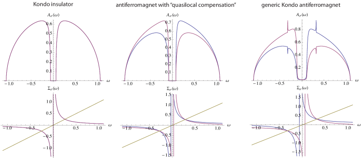
Figure 1: (Color online) Local spectral functions $A_{\sigma}(\omega)$ (top row) computed for self-energies $\Sigma_{\sigma}(\omega)$ (bottom row) approximated by a single pole on or near the real axis for bipartite lattice that allows AFM order. In the Kondo insulator, there is no spin splitting and the pole is located in the center of the gap at $\omega=0$ on the real axis. In the antiferromagnetic state with “quasilocal compensation”, the poles are located symmetrically on the real axis at $\omega=\pm H$ and the real parts of $\Sigma$ are additionally shifted by $\pm h=\mp H$. In generic Kondo antiferromagnet, the values of $h$ and $-H$ are not exactly the same and the poles are shifted away from the real axis (i.e., $\mathrm{Im}\Sigma$ is non-zero).

If the quasilocal compensation, Eq. (21), is violated, there is an avoided crossing between the quasiparticle branches. This should in principle lead to an opening of additional gaps, however, since this is a strongly interacting system, the self-energy has non-zero imaginary part and the pole in Eq. (19) can lie away from the real axis. This immediately implies that there will be some additional structure inside the bands at energies $E=\pm\omega^{*}$ where $\omega^{*}$ is now approximately (assuming $h\approx-H$)

$$\omega^{*}\approx\sqrt{h^{2}+{\tilde{V}}^{2}}.$$ (22)

We show in the following that the combination of inelastic scattering (broadening) and the avoided crossings of quasiparticle bands result in asymmetric resonance curves in the local spectral functions (“spin resonances”), as shown in the schematic plots in Fig. 1.

These analytical considerations thus suggest that fine structures are expected quite generically in the DMFT solution. In previous DMFT(QMC), they were not visible, presumably due to difficulties in performing analytic continuations. As we show in the following section, they can be resolved using the DMFT(NRG) approach.

IV DMFT results

IV.1 Spin resonance structures

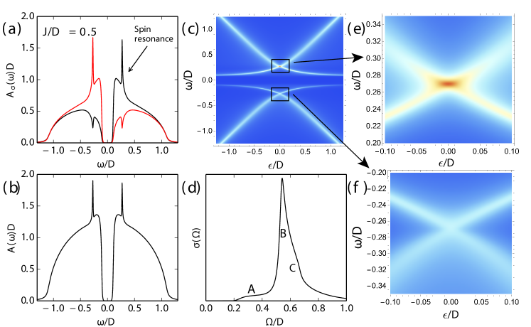
Figure 2: (Color online) Multiple manifestations of the “spin resonance” (fine structure inside the bands) in the dynamical properties of the Kondo lattice model in the antiferromagnetic phase: (a) Peaks and dips in the spin-resolved local spectral function $A_{\sigma}(\omega)$ of the conduction band. (b) Peaks in the spin-averaged local spectral function $A(\omega)=A_{\uparrow}(\omega)+A_{\downarrow}(\omega)$. (c) Momentum-resolved spectral function $A(\epsilon,\omega)$ and close-ups on the regions at $\epsilon=0$ showing (e) an enhanced density of states in the empty band (associated with the resonance) and (f) a reduced density of states, i.e., avoided crossing, in the occupied band (associated with the dip). (d) Optical conductivity exhibiting a hump for energies slightly above the main maximum. Labels (A), (B), and (C) are discussed in the text.

In Fig. 2 we summarize the main results of this work for a value of $J$ in the parameter range where the effects are the most pronounced, i.e., in the strong-coupling case near the AFM-KI transition. In the spectral function of the $c$-band electrons, we observe an additional structure inside the band, Fig. 2(a). In the occupied band, there is a dip for minority spin and a sharp peak for majority spin; the resonance is also visible in the spin-averaged spectral function, $A=A_{\downarrow}+A_{\uparrow}$ shown in Fig. 2(b). The origin of these features can be traced back to the behavior of the momentum-resolved spectral function $A({\mathbf{k}},\omega)$, plotted as a function of $\epsilon_{\mathbf{k}}$ in Fig. 2(c). The close-ups on the regions where the quasiparticle branches should intersect reveal that the spectral dip is associated with a reduced spectral weight between the branches, i.e., an avoided crossing, Fig. 2(f), while the peak corresponds to an enhancement between two branches, Fig. 2(e).

The optical conductance, $\sigma(\Omega)$ shown in Fig. 2(d), shows a threshold at twice the indirect gap $\Delta$, then remains roughly constant up to a sizeable peak at $\Omega\approx 2\omega^{*}$, where transitions between two pairs of bands are strongly enhanced due to the cross-shaped momentum-resolved spectral functions for both occupied and empty bands. The presence of the spin-resonance is reflected in the shape of this peak which has a notable hump in its high-frequency flank.

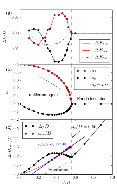
Figure 3: (Color online) From weak-coupling to strong-coupling antiferromagnetism in the Kondo lattice model as a function of the Kondo exchange coupling $J$. a) Reduction of kinetic viz. potential energy with respect to the reference paramagnetic state, indicating different mechanisms of magnetic ordering for weak and strong coupling regimes. b) Staggered magnetization of the conduction band electrons ($m_{c}$) and local moments ($m_{f}$). c) Spectral gap $\Delta$ and spin-resonance position $\omega_{sr}$. $\omega_{sr}$ is not well defined for $J/D\lesssim 0.3$.

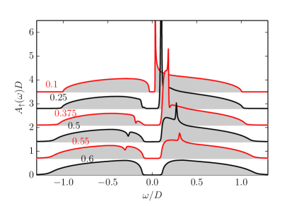
Figure 4: (Color online) Spin-resolved spectral functions of the conduction band for a range of $J$: (a) weak-coupling Slater regime with inverse square root divergence at gap edges ($J/D=0.1$, $0.25$), (b) cross-over regime with a complex form of the spectra near the gap edges ($0.375$), (c) strong-coupling regime with smooth gap edges and well-developped spin resonances ($0.5$, $0.55$), (d) Kondo insulator with no spin resonance ($0.6$).

IV.2 Single-particle properties

The origin of antiferromagnetism in the KLM depends on the value of the exchange coupling $J$, see Fig. 3(a). For small $J$, the AFM order develops by a mechanism similar to the Slater antiferromagnetism in the Hubbard model (although in the KLM, the system would be insulating even in the absence of the unit cell doubling and consequent gap opening due to magnetic order). This regime can be fully explained within a simple Hartree-Fock (HF) theory Rozenberg (1995): the $f$ states are fully polarized, while the $c$ states weakly anti-align with the $f$ spins at each site, Fig. 3(b). There are inverse square root Slater singularities at the gap edges, Fig. 4 for $J/D=0.1$. The quasiparticle gap is linear in $J$ due to the nesting instability ($\epsilon_{k_{F}+q}=-\epsilon_{-k_{F}+q}$) to AFM order in the p-h symmetric case Capponi and Assaad (2001), leading to $\Delta=Jm_{f}$, where $m_{f}$ is the staggered magnetization of the $f$ orbitals. The $f$ spins are nearly fully polarized ($m_{f}\to 1/2$ as $J\to 0$), while $c$ electrons start out unpolarized ($m_{c}\to 0$ as $J\to 0$).

In the intermediate regime, $J\sim J^{\prime}\approx 0.4D$, the spin resonance gradually develops from the band edge, Fig. 4. In this regime, the gap vs. $J$ curve flattens out to form a broad plateau that peaks around $J/D=0.35$. The staggered magnetization of the conduction-band electrons is also maximal in this parameter range.

For $J>J^{\prime}$, in the strong-coupling regime, the AFM is driven by the reduction in the kinetic energy and is characterized by a well-resolved spin resonance, Fig. 4(c). The staggered magnetizations $m_{c}$ and $m_{f}$, as well as the gap $\Delta$ are all decreasing in this regime. Finally, as $J$ is increased further, there is a second-order quantum phase transition to a paramagnetic Kondo insulator state, Fig. 4(d). The charge gap is continuous across the transition.

In the intermediate to strong-coupling regime, the band gap $\Delta$ is non-linear, even non-monotonous, function of $J$, while the spin resonance position $\omega_{sr}$ behaves linearly, see Fig. 3(c). A good fit is given by

$$\omega_{sr}=0.717J-0.089.$$ (23)

This linearity is “inherited” from the Kondo insulator phase, where it holds for the quantity $\omega^{*}$. This further emphasizes the continuous nature of the AFM-KI phase transition and the persistence of itinerancy.

IV.3 Optical conductivity

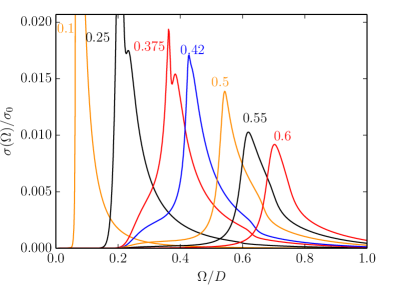
Figure 5: (Color online) Optical conductivity for a range of $J/D$ (as indicated in the plot next to the corresponding curves). Weak-coupling antiferromagnetism is characterized by threshold behavior with a peak at $2\Delta$, while strong-coupling antiferromagnetism exhibits more complex behavior with threshold at $2\Delta$ and the main peak at $2\omega^{*}\approx 2\omega_{\mathrm{sr}}$, the spin resonance appearing as a secondary maximum or as a hump on the flank of the main peak. $\sigma_{0}=e^{2}/h$.

In the weak-coupling AFM regime, the optical conductivity shows a threshold behavior with a pronounced resonance corresponding to twice the quasiparticle gap, $\Omega=2\Delta$, see Fig. 5 for $J/D=0.1$. Similar behavior is also observed in the Slater AFM regime of the Hubbard model Zitzler et al. (2002). In the strong-coupling regime, the curves are more complex, Fig. 2(d). After the threshold at $\Omega=2\Delta$, there is (A) a region of moderate conductivity, followed by (B) a pronounced resonance at $\Omega=2\omega^{*}$, and (C) an additional more-or-less pronounced structure associated with the spin-resonance. As $J$ is increased toward $J_{c}$, region A progressively flattens out and evolves into a plateau of nearly constant very low optical conductivity (see $J/D=0.375$, $0.42$, and $0.50$ in Fig. 5). This region is associated with the transitions between the quasiparticles at band edges ($\epsilon_{\mathbf{k}}\approx\pm D$) which have low spectral weight. Region B is associated with the cross-shaped form of the $\epsilon_{\mathbf{k}}$-resolved spectral function in the band-center ($\epsilon_{\mathbf{k}}\approx 0$).

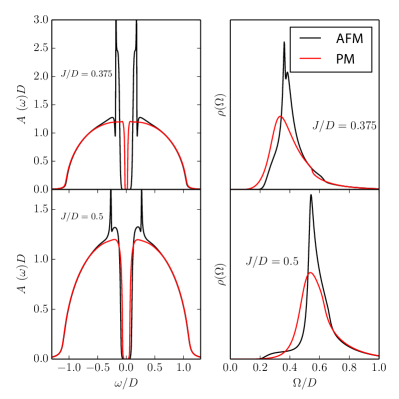
Figure 6: (Color online) Comparison of antiferromagnetic and paramagnetic DMFT solutions for equal values of $J$ reveals the fine details in the ordered phase.

It is worth to emphasize that the spin resonances are not observed for negative (ferromagnetic) Kondo exchange coupling $J$, although the system is also antiferromagnetic. This is due to the very different topology of the quasiparticle bands (“small Fermi surface”) in this case Hoshino et al. (2010); Bodensiek et al. (2011b), which is, in turn, associated with a different form of the self-energy function with no pronounced poles. Furthermore, there is no spin resonance if we enforce paramagnetic solution in the region where the AFM is the true ground state (such a comparison of AFM and PM solutions in shown in Fig. 6); in the paramagnetic case the topology is that of “large Fermi surface”, but there is no staggered magnetization. We thus conclude that the spin resonance is a characteristic property of itinerant antiferromagnetism, requiring both itinerancy of $f$ electrons and staggered magnetization.

In DMFT calculations using solvers requiring an analytical continuation, such in-band spectral features have not been observed. This is the case also for high-quality continuous-time QMC calculations Hoshino et al. (2010). Some hints of the spin resonances have been observed in prior DMFT(NRG) works Peters and Pruschke (2007b); Peters et al. (2011); Bodensiek et al. (2011b), but have not been discussed. The spin resonances appear for any value of the NRG broadening parameter: even in calculation with no $z$-averaging and with large broadening parameter their presence is suggested by a broad spectral hump in one band and as a faint depression in the other. As the broadening is decreased, these features become sharper and more asymmetric. Because of their persistent nature and very generic conditions on the functional form of the self-energy for their emergence, it is unlikely that they were a numerical artifact of NRG calculations.

IV.4 Temperature dependence

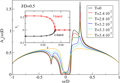
Figure 7: (Color online) Reduction of the spin resonance structure (peak weight) with increasing temperature. Inset: temperature variation of the staggered magnetization across the thermal AFM-PM phase transition.

The staggered magnetization decreases with increasing temperature until at the Néel temperature $T_{N}$ the system undergoes a transition to the paramagnetic phase, Fig. 7. The evolution of the spectra confirms the relation of the spin-resonance peaks with the magnetic order, since the peak intensity follows the staggered magnetization. Interestingly, the peak position itself does not depend much on the order parameter. It is also noteworthy that the overall structure of the effective bands does not change accross the transition Hoshino et al. (2010). A sign of this is the persistence of a reduced density of states (a hybridization-induced “pseudo-gap”) around $\omega=0$ to temperatures well above $T_{N}$, where the order parameter is already zero and the spin resonance structure eliminated.

IV.5 Magnetic field

We now consider the effect of an external magnetic field on the antiferromagnetic state. We assume $g\equiv g_{c}=g_{f}$ and express the field in units of the Zeeman energy, $g\mu_{B}B$. There are no magnetic anisotropy terms in our Hamiltonian, thus in the ground state the staggered magnetization always reorients itself perpendicular to the applied field to preserve the exchange energy generated by the antialignment of spins in $c$ and $f$ bands. Likewise, when magnetic field is applied on the Kondo insulator, it induces an antiferromagnetic phase transverse to the external field Beach et al. (2004); Ohashi et al. (2004). In this work we will follow the convention that the direction of the field is taken to be along the $x$ axis (we denote this as the “longitudinal” direction) and the staggered magnetization along the $z$ axis (this is the “transverse” direction).

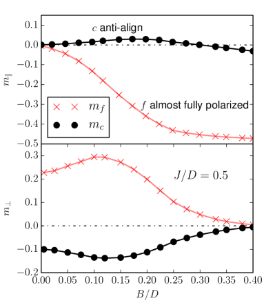
Figure 8: (Color online) Effect of an applied magnetic field on the magnetic order in the antiferromagnetic phase of the Kondo lattice model. Upper panel: uniform magnetization components $m_{\parallel}$ of $c$ and $f$ orbitals in the direction of the field. Bottom panel: staggered magnetization components $m_{\perp}$ of $c$ and $f$ orbitals perpendicular to the field. The following defining relations hold: $m_{x,A}=m_{x,B}=m_{\parallel}$ and $m_{z,A}=-m_{z,B}=m_{\perp}$.

$f$ electrons have higher magnetic susceptibility than $c$ electrons, thus their uniform magnetization rapidly increases with the applied field, while the $c$ electrons at first anti-align due to the strong local Kondo coupling $J\gg B$ and only for very strong fields (of order $J$) reorder in the same direction as the $f$ orbitals, see upper panel in Fig. 8. For weak fields, the stagerred magnetization first increases, see lower panel in Fig. 8. This can be explained as the suppression of the Kondo effect by breaking the local singlets through magnetic field, which leads to stronger spin polarization of the orbitals. The staggered magnetization is maximal for $B=B_{m}\approx 0.1D$ and then slowly decreases towards $0$ as the gap is closing. The charge gap becomes exponentially small in the large-$B$ limit Beach et al. (2004), thus at non-zero temperature the system is effectively a strongly spin-polarized paramagnetic metal. The results in Fig. 8 can be qualitatively reproduced using a simple exact calculation on a two-site cluster with suitable molecular fields for AFM order put in by hand. The only small discrepancies are due to the stronger itinerancy of $c$ electrons in the full latice.

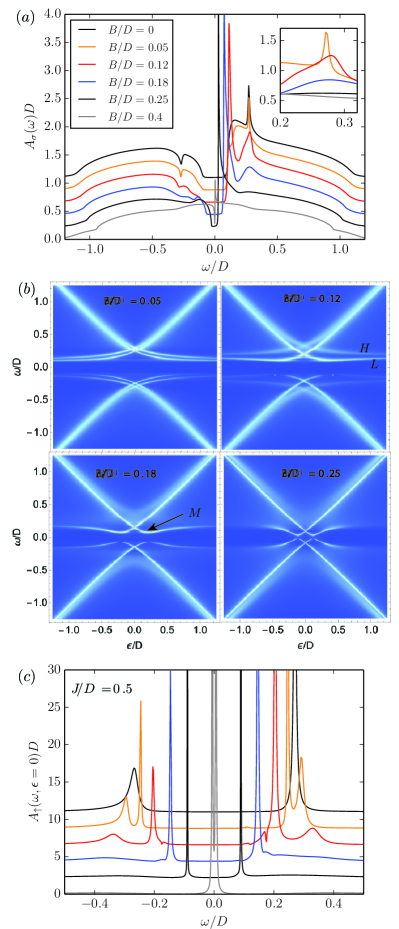
Figure 9: (Color online) Evolution of (a) local spectral function $A_{\sigma}(\omega)$ and (b) momentum-resolved spectra $A_{\sigma}(\epsilon_{\mathbf{k}},\omega)$ for increasing external magnetic field $B$ in the strong-coupling AFM phase ($J/D=0.5$). Labels L, H, and M are explained in the text. The cross-cut of the momentum-resolved spectrum at $\epsilon=0$ is shown in panel (c).

The spectra undergo significant changes as the field is applied, see Fig. 9. Local spectral functions (top panel) reveal that the spin resonances are resilient to small fields and that their position remains roughly constant as $B$ is increased. They are washed away at higher fields when the AFM order itself becomes strongly suppressed. This is in line with the interpretation of the spin resonance as a manifestation of the staggered magnetization. The width of the resonances is, however, strongly field dependent, reaching a maximum for values of order $B_{m}$ where the staggered magnetization peaks. When $B$ increases further, the resonance is suppressed at the same time as the staggered magnetization tends toward 0, as expected. The behavior of spectral functions near the band edges is equally interesting. In particular, we note the reemergence of the structure characteristic for the weak-coupling case with square-root and inverse-square-root singularities.

The field-dependence can be better understood through the momentum-resolved spectral functions, see panel (b) in Fig. 9. In weak field, the main effect is the “doubling” of the quasiparticle branches (four to eight). This results from the breaking of the symmetry relation $G_{A\sigma}(\omega)=G_{B\bar{\sigma}}(\omega)$ which guarantees the degeneracy of the branches in the absence of the external field. Physically, this means that in the presence of the field the $c$ band electrons propagate slightly differently if their spin has a transverse component which is aligned or antialigned with the uniform component of the magnetization. This difference becomes more pronounced at larger fields, and the splitting grows larger (see the case of $B/D=0.12$). We also note that the higher-energy branches (label H in the plot) always have much shorter quasiparticle lifetime than the lower-energy ones (label L in the plot) because of the relaxation mechanism via transverse spin component reorientation, taking the quasiparticles from the upper to the lower branch. At high fields the H branches become so diffuse that they can hardly be distinguished. This evolution can also be followed in the constant-momentum section of the momentum-resolved spectrum shown in Fig. 9(c).

A further effect of the field is the emergence of the curvature in the L branches, see label M in Fig. 9(b). This new feature directly explains the resurgence of the (inverse)-square-root singularities at the gap edges, since the direct gap moves from the non-interacting band edges at $\epsilon=\pm D$, where the DOS goes to zero, $\rho(\pm D)=0$, to inner regions, gradually shifting to the center of the band at $\epsilon=0$ as $B$ increases.

In Sec. V we will see that most of these features can be explained in the hybridization picture with longitudinal uniform and transverse staggered magnetization.

IV.6 Universality and robustness

It has been pointed out that in the DMFT the most important characteristic of the non-interacting density of states (DOS) of the lattice is its effective bandwidth, defined through the second moment of the DOS,

$$D_{\mathrm{eff}}=\int\,\epsilon^{2}\rho_{0}(\epsilon)\mathrm{d}\epsilon,$$ (24)

which sets the scale of the kinetic energy. It is equal to $D$ for the Bethe lattice and 2D cubic (square) lattice, $0.816D$ for 3D cubic lattice, and $1.41D$ for the hypercubic lattice. Indeed, it has been found that the Mott metal-insulator-transition at $T=0$ in the paramagnetic phase of the Hubbard model occurs at roughly the same value of the rescaled electron-electron repulsion parameter $U/D_{\mathrm{eff}}$, which reflects the nature of the transition: competition between the delocalizing effect of the kinetic energy and the localizing effect of the electron-electron repulsion.

For the AFM-KI phase transition in the KLM, we also find that the critical coupling is given by essentially the same ratio of $J_{c}/D_{\mathrm{eff}}$ (we obtain $J_{c}/D_{\mathrm{eff}}\approx 0.56$ for the Bethe lattice, 2D and 3D cubic, and $J_{c}/D_{\mathrm{eff}}\approx 0.54$ for the hypercubic lattice). This can again be rationalized in terms of a competition between kinetic and exchange terms: kinetic terms promote delocalization of $c$ electrons, while the exchange terms enhance their localization by generating localized Kondo singlet states. This essentially agrees with Doniach’s picture of competing RKKY and Kondo ground states.

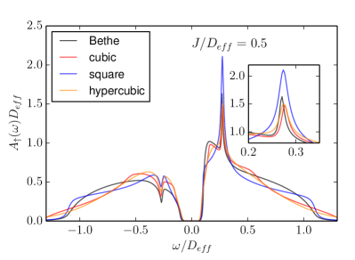
Figure 10: (Color online) Spectral functions of the Kondo lattice model on four different lattices: Bethe lattice, 2D cubic (square lattice), 3D cubic, and infinite-D cubic (Gaussian DOS) lattices. Note that the figure axes are scaled in terms of the effective bandwidth $D_{\mathrm{eff}}$ and that the same rescaled parameter $J/D_{\mathrm{eff}}$ has been used in all four DMFT calculations.

The scaling in terms of $D_{\mathrm{eff}}$ is valid even more generally. The comparison of spectral functions computed for different lattice types, Fig. 10, shows that despite significant differences in details, the main features of appropriately rescaled spectral functions are common to all cases: a) they have essentially the same quasiparticle gap $\Delta$, b) they exhibit a spin resonance structure, and c) the spin resonance appears at roughly the same frequency $\omega_{sr}$ and has comparable spectral weight (with the exception of square lattice which has a van Hove singularity at $\epsilon=0$ that enhances the spin resonance peak).

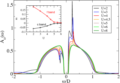
Figure 11: (Color online) In periodic Anderson model (PAM), if $J\propto t^{2}/U$ is kept constant while $t$ and $U$ increase, the AFM order is suppressed, the spin resonance disappears, yet the gap remains constant.

The spin resonance is also present in closely related models which have itinerant AFM order: high-spin Kondo lattice model (explicitly tested for $S=1$ KLM, also in presence of magnetic anisotropy term $DS_{z}^{2}$, for both axial $D<0$ and planar $D>0$ anisotropy) and the periodic Anderson model (PAM) with parameters chosen so that the model is particle-hole symmetric and in the Kondo limit (large $U$ and $\epsilon+U/2=0$). In PAM, if hybridization $t$ and $f$-level charge repulsion $U$ are increased while keeping the effective Kondo coupling $J\propto t^{2}/U$ constant, the hybridization is increased in comparison with the exchange energy. The result is that the staggered magnetization decreases and the spin resonance gradually disappears, yet the spectral gap remains roughly constant, see Fig. 11. Interestingly, as $t$ increases at constant $J$, the charge fluctuations on the $f$ level actually decrease due to increasing $U$.

V Discussion

The DMFT results indicate that at half filling the hybridization picture is an essentially correct description of the antiferromagnetic phase of the Kondo lattice model and that the topology of the quasiparticle bands remains the same (large Fermi surface) for all values of $J$. At the same time, our numerical results indicate that at the quantitative level there are interesting details that have experimentally observable consequences, such as the presence of enhanced and suppressed density of states in the centre of the band at the avoided crossing points of the quasiparticle bands (visible in ARPES) and the non-trivial structure of the optical conductivity (see, in particular, the comparison in Fig. 6). The hybridization picture does not include any inelastic-scattering processes, since it is essentially a non-interacting theory. Even at $T=0$ it therefore does not properly capture effects away from the Fermi level, but nevertheless it is a good starting point.

Let us first analyze the equation for the quasiparticle bands,

$$\mathrm{Re}[\zeta_{A\sigma}(\omega)\zeta_{B\sigma}(\omega)-\epsilon^{2}]=0,$$ (25)

focusing on the region close to the spin resonance at $\epsilon=0$. We are then actually solving

$$\mathrm{Re}[(\omega-\Sigma_{\uparrow}(\omega))(\omega-\Sigma_{\downarrow}(\omega))]=0.$$ (26)

Neglecting the imaginary parts of $\Sigma$, this reduces to

$$(\omega-\mathrm{Re}\Sigma_{\uparrow}(\omega))(\omega-\mathrm{Re}\Sigma_{\downarrow}(\omega))]=0,$$ (27)

and it follows that the solutions are given by

$$\omega=\mathrm{Re}\Sigma_{\sigma}(\omega).$$ (28)

It turns out that in the range of $J$ where the spin resonance is the most pronounced, this equation has solutions at $\omega\approx\pm\omega_{\mathrm{sr}}$ for both spin directions. In other words, one has

$$\mathrm{Re}\Sigma_{\uparrow}(\omega_{\mathrm{sr}})\approx\mathrm{Re}\Sigma_{\downarrow}(\omega_{\mathrm{sr}})\approx\omega_{\mathrm{sr}}.$$ (29)

This condition has been interpreted in Ref. Hoshino et al., 2010 in terms of the molecular fields $h$ and $H$ as the relation $h=-H$ and named the “quasilocal compensation”. We find, however, that this “compensation” is not generally valid.

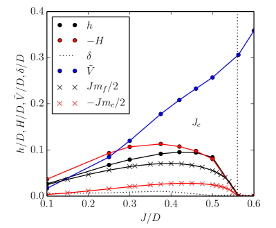
Figure 12: (Color online) Kondo antiferromagnet in the hybridization picture with spin polarization: parameters for the single-pole Ansatz for the self-energy $\Sigma_{\sigma}(\omega)$ as a function of the Kondo coupling $J$.

We have systematically extracted the parameters from the calculated self-energy functions using the following hybridization-picture Ansatz:

$$\Sigma_{\uparrow}(\omega)=h+\frac{\tilde{V}^{2}}{z-H+i\delta}.$$ (30)

A small imaginary part $\delta$ has been added to account for the finite width of the peak in $\mathrm{Im}\Sigma$. For stability, the parameter extraction has been performed simultaneously on real and imaginary parts of the function. The results are shown in Fig. 12. The plot reveals that the curves $h(J)$ and $-H(J)$ have a similar non-monotonic behavior with a maximum value in the cross-over region between the weak- and strong-coupling antiferromagnet, but they intersect at a single plot near $J/D=0.5$. The hybridization parameter $\tilde{V}$ is continuous across the AFM-KI transition, as already noted in Ref. Hoshino et al., 2010. The imaginary-part parameter $\delta$ is small, but needs to be included for a good fit, even though it leads to worse agreement with $\mathrm{Im}\Sigma(\omega)$, which, in particular, should be strictly equal to zero inside the gap.

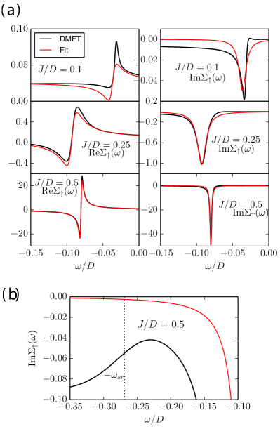
Figure 13: (Color online) Self-energy functions and fits to the hybridization-picture Ansatz with a single-pole. The fit quality is mediocre in the weak-coupling regime ($J/D=0.1$), but improves in the strong-coupling regime ($J/D=0.5$). (b) $\mathrm{Im}\Sigma$ has some fine structure in addition to the dominant poles.

In Fig. 13(a) we plot the real and imaginary parts of the self-energy together with the corresponding single-pole fit functions. The agreement is better in the strong-coupling regime at $J/D=0.5$ where the pole is very strong and dominates the remaining structure in the self-energy, visible in the close-up on $\mathrm{Im}\Sigma(\omega)$ shown in panel (b) and labeled as B. Surprisingly, in the weak-coupling regime at $J/D=0.1$, the agreement is much less satisfactory. The main reason is that the pole is not much larger compared with the remaining structure: region B is merged with the pole A, thus the peak is no longer a simple Lorentzian and consequently $\mathrm{Re}\Sigma(\omega)$ is asymmetric.

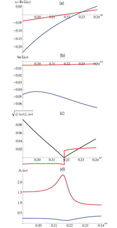
Figure 14: (Color online) Analytical structure leading to the spin resonance. a) Nearby solutions of $\omega=\mathrm{Re}\Sigma_{\sigma}(\omega)$ for $\sigma=\uparrow$ and $\sigma=\downarrow$. b) $\mathrm{Im}\Sigma_{\sigma}(\omega)$ are nearly constant for $\omega\approx\omega_{\mathrm{sr}}$. c) Argument of the non-interacting Green’s functions in the DMFT expression (Eq. (17)) for local Green’s functions. d) Resulting local spectral functions featuring enhancement or suppression at $\omega\approx\omega_{\mathrm{sr}}$.

We emphasize that the spin resonances are not located at the frequencies of the poles in the self-energy, but at significantly higher energies. We now study this in more detail by considering the generic case at $J/D=0.4$ where $h$ and $-H$ differ slightly. Functions $Re\zeta_{A\sigma}(\omega)=\omega-\mathrm{Re}\Sigma_{A\sigma}(\omega)$ intersect the real axis at two different points, see Fig. 14(a). Somewhere between these two points, the function $p=(\zeta_{A\sigma}(\omega)\zeta_{B\sigma}(\omega))^{1/2}$ goes through a branch cut so that its imaginary part has a jump, Fig. 14(c). This discontinuity is canceled by that in $G_{0}(p)-G_{0}(-p)$, resulting in a continuous spectral function, which however has a peak, Fig. 14(d).

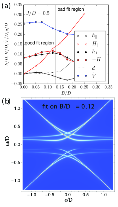
Figure 15: (Color online) a) Parameters for the hybridization-picture Ansatz for the Kondo antiferromagnet in external magnetic field. b) Momentum-resolved spectral function at finite magnetic field.

We now consider the case of finite magnetic field where the momentum-resolved spectral functions show complex structure with quasiparticle branch doubling in number. The simplest attempt to rationalize this behavior is to incorporate the additional uniform magnetic field in the hybridization picture. The self-energy function now has a $2\times 2$ matrix structure:

$$\bm{\Sigma}(\omega)=\begin{pmatrix}h_{\perp}&h_{\|}\\ h_{\|}&-h_{\perp}\end{pmatrix}+\tilde{V}^{2}\left(z-\begin{pmatrix}H_{\perp}&H_{\|}\\ H_{\|}&-H_{\perp}\end{pmatrix}+i\delta\right)^{-1}.$$ (31)

The extracted parameters are shown in Fig. 15. The staggered components $h_{\perp}$ and $H_{\perp}$ (which correspond to the previously discussed $h$ and $H$ in the absence of the field) have only weak $B$ dependence: at first they slightly grow (in absolute value), similar to the staggered magnetization components $m_{c\perp}$ and $m_{f\perp}$, then decrease. The homogeneous longitudinal molecular field components also mimick the corresponding magnetization components: $H_{\|}$ rapidly grows with $B$ and eventually becomes the dominant molecular field, while $h_{\|}$ slightly increases and then changes sign. The effective hybridization $\tilde{V}$ does not change appreciably with field. We also note that the quality of the fit worsens at high fields. This is expected since the systems renormalizes toward a weakly-interacting spin-polarized limit where the simple hybridization picture is not a good approximation (similar to the case of small $J$ at $B=0$).

It is worth mentioning that in the strong-coupling regime for large $J/D\sim 0.5$, $\tilde{V}$ is much larger than $h\approx-H$, thus $\omega^{*}=\sqrt{\tilde{V}^{2}+h^{2}}\sim\tilde{V}$. The effective hybridization $\tilde{V}$ is not strongly affected by the field, therefore $\omega^{*}$ remains approximately constant. This explains why the spin resonance position is not much affected by the external magnetic field, as seen in Fig. 9.

VI Conclusion

We have performed a detailed study of the spectral properties of the Kondo lattice model at half-filling where the system is an itinerant antiferromagnetic insulator for $J<J_{c}$ and a paramagnetic Kondo insulator for $J>J_{c}$. The dynamical mean-field theory calculations have been performed with a quantum impurity solver with high spectral resolution. We have uncovered fine structure (“spin resonances”) inside the bands at frequencies given by the crossing point of the quasiparticle branches in the centre of the non-interacting band ($\epsilon=0$). These features are due to the inelastic-scattering processes which are not taken into account in the simplified hybridization picture. They are directly related to the existence of the AFM order: whenever the AFM order disappears, either due to thermal phase transition, external magnetic field, or quantum phase transition to the KI, the spin resonances also disappear.

Similiar spin resonances also exist in the superconducting phase of the KLM Bodensiek et al. (2013) and they share some other common properties, for instance their position also changes linearly with $J$. These analogies are not too surprising since the Nambu formalism used to describe superconductivity is very similar to the A/B sublattice formalism used to describe Néel order on bipartite lattices, thus the analytical structure of the DMFT self-consistency equations is analogous. Following this analogy, the resonances in the superconducting case can be interpreted to be arising from simultaneous presence of the $f$-electron itinerancy (heavy Fermi liquid) and non-zero order parameter, and should thus appear generically in heavy-fermion $s$-wave superconductors. This is a further indication that the superconducting state emerges out of the large Fermi surface heavy fermion state.

The most direct way to experimentally observe such sharp spectral structure is tunneling spectroscopy which gives access to local spectral function where the “spin resonance” is the most pronounced (more than in the momentum-resolved spectral functions measurable by ARPES). The feature to look for is the apparition of an antisymmetric resonance at finite frequencies as the system becomes antiferromagnetic, with an intensity directly related to the order parameter. Another possibility is optical spectroscopy where fine details of peak shapes can also be easily measured.

The effect of non-local correlations on the observed fine structure remains an open question and will be a part of future research. It could be addressed, for instance, in cellular DMFT studies Tanasković et al. (2011).

Appendix A DMFT(NRG) approach in the absence of spin symmetries

The inverse Green’s function has a block $2\times 2$ matrix structure, each block being itself a $2\times 2$ matrix in the spin space:

$$G_{k}^{-1}(z)=\begin{pmatrix}z+\mu-\tau^{3}(h+h_{s})-\tau^{1}h_{t}-\Sigma_{A}&-\epsilon_{k}\\ -\epsilon_{k}&z+\mu-\sigma^{3}(h-h_{s})-\tau^{1}h_{t}-\Sigma_{B}\end{pmatrix}.$$ (32)

Here $\tau^{i}$ are Pauli matrices, $h_{s}$ is the staggered field, $h$ is the longitudinal homogeneous field and $h_{t}$ is the homogenous transverse field. As in the spin diagonal case, we introduce $\zeta_{A}$ and $\zeta_{B}$,

$$G_{k}^{-1}(z)=\begin{pmatrix}\zeta_{A}&-\epsilon_{k}\\ -\epsilon_{k}&\zeta_{B}\end{pmatrix}.$$ (33)

We assume $\zeta_{A}$ and $\zeta_{B}$ to be invertible, and perform a blockwise invertion of the matrix:

$$M=\begin{pmatrix}A&B\\ C&D\end{pmatrix}\quad\leftrightarrow M^{-1}=\begin{pmatrix}(A-BD^{-1}C)^{-1}&-A^{-1}B(D-CA^{-1}B)^{-1}\\ -D^{-1}C(A-BD^{-1}C)^{-1}&(D-CA^{-1}B)^{-1}\end{pmatrix}$$ (34)

thus

$$G_{k}(z)=\begin{pmatrix}(\zeta_{A}-\epsilon_{k}^{2}\zeta_{B}^{-1})^{-1}&{\ldots}\\ {\ldots}&(\zeta_{B}-\epsilon_{k}^{2}\zeta_{A}^{-1})^{-1}.\end{pmatrix}$$ (35)

The out-of-diagonal elements are of no interest, because they are odd functions of $\epsilon_{k}$ and will drop out after the integration since $D(\epsilon)$ is assumed to be even (It is indeed even for all lattice types considered in this work).

The local Green’s function is

$$G(z)=\frac{1}{N}\sum_{k}G_{k}(z)=\int d\epsilon D(\epsilon)\begin{pmatrix}\zeta_{B}(\zeta_{A}\zeta_{B}-\epsilon^{2})^{-1}&{\ldots}\\ {\ldots}&\zeta_{A}(\zeta_{B}\zeta_{A}-\epsilon^{2})^{-1}\end{pmatrix}.$$ (36)

Note that $\zeta_{A}$ and $\zeta_{B}$ in general do not commute.

We consider each diagonal submatrix problem. We write

$$F^{A}=\zeta_{A}\zeta_{B},\quad F^{B}=\zeta_{B}\zeta_{A}$$ (37)

and

$$D^{A}=F^{A}-\epsilon^{2},\quad D^{B}=F^{B}-\epsilon^{2}.$$ (38)

We need to integrate each matrix component separately, but the pole structure is the same for all components.

We write

$$F^{A}=\begin{pmatrix}F_{11}&F_{12}\\ F_{21}&F_{22}\end{pmatrix}$$ (39)

and

$$D^{A}=\begin{pmatrix}F_{11}-\epsilon^{2}&F_{12}\\ F_{21}&F_{22}-\epsilon^{2}\end{pmatrix}.$$ (40)

Then

$$[D^{A}]^{-1}=\frac{1}{(F_{11}-\epsilon^{2})(F_{22}-\epsilon^{2})-F_{12}F_{21}}\begin{pmatrix}F_{22}-\epsilon^{2}&-F_{12}\\ -F_{21}&F_{11}-\epsilon^{2}\end{pmatrix}.$$ (41)

We expand the fraction:

$$\frac{1}{(F_{11}-\epsilon^{2})(F_{22}-\epsilon^{2})-F_{12}F_{21}}=c^{A}\left[\frac{1/\epsilon_{1}}{\epsilon-\epsilon_{1}}+\frac{-1/\epsilon_{1}}{\epsilon+\epsilon_{1}}+\frac{-1/\epsilon_{2}}{\epsilon-\epsilon_{2}}+\frac{1/\epsilon_{2}}{\epsilon+\epsilon_{2}}\right],$$ (42)

where

$$\epsilon_{1,2}=\frac{1}{\sqrt{2}}\left(F_{11}+F_{22}\pm\sqrt{F_{11}^{2}+F_{22}^{2}+4F_{12}F_{21}-2F_{11}F_{22}}\right)^{1/2}$$ (43)

and

$$c^{A}=\frac{1/2}{(\epsilon_{1}-\epsilon_{2})(\epsilon_{1}+\epsilon_{2})}.$$ (44)

We use the relation

$$\int\frac{D(\epsilon)\epsilon^{2}d\epsilon}{z-\epsilon}=-z+z^{2}\int\frac{D(\epsilon)d\epsilon}{z-\epsilon}=-z+z^{2}G^{0}(z)$$ (45)

where $G^{0}(z)$ is the non-interacting local Green’s function for the chosen lattice problem. Thus, for example

$$\int\frac{D(\epsilon)d\epsilon}{\epsilon-\epsilon_{1}}=-G^{0}(\epsilon_{1}),$$ (46)

and

$$\int\frac{\epsilon^{2}D(\epsilon)d\epsilon}{\epsilon-\epsilon_{1}}=\epsilon_{1}-\epsilon_{1}^{2}G^{0}(\epsilon_{1}).$$ (47)

Then

$$G(z)=\int d\epsilon D(\epsilon)\begin{pmatrix}\zeta_{B}[D^{A}]^{-1}&{\ldots}\\ {\ldots}&\zeta_{A}[D^{B}]^{-1}\end{pmatrix}=\begin{pmatrix}\zeta_{B}J^{A}&0\\ 0&\zeta_{A}J^{B}\end{pmatrix},$$ (48)

where $J^{A/B}$ are the integrals over $\epsilon$. Since $\zeta_{A/B}$ depend only on $z$, not $\epsilon$, they may be factored out and taken into account after the integration.

For $J^{A}$ we find

$$\begin{split}J^{A}&=c^{A}\begin{pmatrix}F_{22}&-F_{12}\\ -F_{21}&F_{11}\end{pmatrix}\left[-(1/\epsilon_{1})G^{0}(\epsilon_{1})+(1/\epsilon_{1})G^{0}(-\epsilon_{1})+(1/\epsilon_{2})G^{0}(\epsilon_{2})-(1/\epsilon_{2})G^{0}(-\epsilon_{2})\right]\\ &-c^{A}\begin{pmatrix}1&0\\ 0&1\end{pmatrix}\left\{+(1/\epsilon_{1})[\epsilon_{1}-\epsilon_{1}^{2}G^{0}(\epsilon_{1})]-(1/\epsilon_{1})[-\epsilon_{1}-\epsilon_{1}^{2}G^{0}(-\epsilon_{1})]-(1/\epsilon_{2})[\epsilon_{2}-\epsilon_{2}^{2}G^{0}(\epsilon_{2})]+(1/\epsilon_{2})[-\epsilon_{2}-\epsilon_{2}^{2}G^{0}(-\epsilon_{2})]\right\}.\end{split}$$ (49)

For each $A/B$ subproblem, the hybridization function is then the standard one:

$$\Delta_{i}(z)=\mathrm{Im}\left[G_{i}^{-1}(z)+\Sigma_{i}(z)\right],$$ (50)

with $i=A/B$, and $\Delta_{i}$, $G_{i}$ and $\Sigma_{i}$ are all 2x2 matrices.

References

- Hewson (1997) A. C. Hewson, The Kondo problem to heavy fermions, 2 (Cambridge university press, 1997).
- Stewart (1984) G. R. Stewart, Rev. Mod. Phys. 56, 755 (1984), URL http://link.aps.org/doi/10.1103/RevModPhys.56.755.
- Jaime et al. (2000) M. Jaime, R. Movshovich, G. R. Stewart, W. P. Beyermann, M. G. Berisso, M. F. Hundley, P. C. Canfield, and J. L. Sarrao, Nature 405, 160 (2000).
- Sugiyama et al. (1988) K. Sugiyama, F. Iga, M. Kasaya, T. Kasuya, and M. Date, Journal of the Physical Society of Japan 57, 3946 (1988).
- Mason et al. (1992) T. E. Mason, G. Aeppli, A. P. Ramirez, K. N. Clausen, C. Broholm, N. Stücheli, E. Bucher, and T. T. M. Palstra, Phys. Rev. Lett. 69, 490 (1992).
- Bat’ková et al. (2006) M. Bat’ková, I. Bat’ko, E. Konovalova, N. Shitsevalova, and Y. Paderno, Physica B: Condensed Matter 378–380, 618 (2006).
- Knafo et al. (2010) W. Knafo, D. Aoki, D. Vignolles, B. Vignolle, Y. Klein, C. Jaudet, A. Villaume, C. Proust, and J. Flouquet, Phys. Rev. B 81, 094403 (2010), URL http://link.aps.org/doi/10.1103/PhysRevB.81.094403.
- Degiorgi (1999) L. Degiorgi, Reviews of Modern Physics 71, 687 (1999).
- Wilson (1975) K. G. Wilson, Rev. Mod. Phys. 47, 773 (1975), URL http://link.aps.org/doi/10.1103/RevModPhys.47.773.
- Doniach (1977) S. Doniach, Physica B+ C 91, 231 (1977).
- Hoshino et al. (2010) S. Hoshino, J. Otsuki, and Y. Kuramoto, Phys. Rev. B 81, 113108 (2010).
- Coleman (2006) P. Coleman, eprint arXiv:cond-mat/0612006 (2006), eprint cond-mat/0612006.
- Georges et al. (1996a) A. Georges, G. Kotliar, W. Krauth, and M. J. Rozenberg, Rev. Mod. Phys. 68, 13 (1996a), URL http://link.aps.org/doi/10.1103/RevModPhys.68.13.
- Krishna-murthy et al. (1980) H. R. Krishna-murthy, J. W. Wilkins, and K. G. Wilson, Phys. Rev. B 21, 1003 (1980), URL http://link.aps.org/doi/10.1103/PhysRevB.21.1003.
- Bulla et al. (2008) R. Bulla, T. A. Costi, and T. Pruschke, Rev. Mod. Phys. 80, 395 (2008), URL http://link.aps.org/doi/10.1103/RevModPhys.80.395.
- Peters et al. (2006) R. Peters, T. Pruschke, and F. B. Anders, Phys. Rev. B 74, 245114 (2006), URL http://link.aps.org/doi/10.1103/PhysRevB.74.245114.
- Weichselbaum and von Delft (2007a) A. Weichselbaum and J. von Delft, Phys. Rev. Lett. 99, 076402 (2007a), URL http://link.aps.org/doi/10.1103/PhysRevLett.99.076402.
- Žitko and Pruschke (2009) R. Žitko and T. Pruschke, Phys. Rev. B 79, 085106 (2009), URL http://link.aps.org/doi/10.1103/PhysRevB.79.085106.
- Bodensiek et al. (2011a) O. Bodensiek, R. Žitko, R. Peters, and T. Pruschke, Journal of Physics: Condensed Matter 23, 094212 (2011a).
- Peters and Pruschke (2007a) R. Peters and T. Pruschke, Phys. Rev. B 76, 245101 (2007a), URL http://link.aps.org/doi/10.1103/PhysRevB.76.245101.
- Yoshida et al. (1990) M. Yoshida, M. A. Whitaker, and L. N. Oliveira, Phys. Rev. B 41, 9403 (1990), URL http://link.aps.org/doi/10.1103/PhysRevB.41.9403.
- Bulla et al. (1998) R. Bulla, A. Hewson, and T. Pruschke, Journal of Physics: Condensed Matter 10, 8365 (1998).
- Weichselbaum and von Delft (2007b) A. Weichselbaum and J. von Delft, Phys. Rev. Lett. 99, 076402 (2007b).
- Žitko (2009) R. Žitko, Phys. Rev. B 80, 125125 (2009).
- Taranto et al. (2012) C. Taranto, G. Sangiovanni, K. Held, M. Capone, A. Georges, and A. Toschi, Phys. Rev. B 85, 085124 (2012), URL http://link.aps.org/doi/10.1103/PhysRevB.85.085124.
- Hewson (1993) A. C. Hewson, The Kondo Problem to Heavy-Fermions (Cambridge University Press, Cambridge, 1993).
- Rozenberg et al. (1996) M. J. Rozenberg, G. Kotliar, and H. Kajueter, Phys. Rev. B 54, 8452 (1996).
- Georges et al. (1996b) A. Georges, G. Kotliar, W. Krauth, and M. J. Rozenberg, Rev. Mod. Phys. 68, 13 (1996b).
- Rozenberg (1995) M. J. Rozenberg, Phys. Rev. B 52, 7369 (1995).
- Capponi and Assaad (2001) S. Capponi and F. F. Assaad, Phys. Rev. B 63, 155114 (2001).
- Zitzler et al. (2002) R. Zitzler, T. Pruschke, and R. Bulla, Eur. Phys. J. B 27, 473 (2002).
- Bodensiek et al. (2011b) O. Bodensiek, R. Žitko, R. Peters, and T. Pruschke, J. Phys.: Condens. Matter p. 094212 (2011b).
- Peters and Pruschke (2007b) R. Peters and T. Pruschke, Phys. Rev. B 76, 245101 (2007b).
- Peters et al. (2011) R. Peters, N. Kawakami, and T. Pruschke, Journal of Physics: Conference Series 320, 012057 (2011).
- Beach et al. (2004) K. S. D. Beach, P. A. Lee, and P. Monthoux, Phys. Rev. Lett. 92, 026401 (2004), URL http://link.aps.org/doi/10.1103/PhysRevLett.92.026401.
- Ohashi et al. (2004) T. Ohashi, A. Koga, S.-i. Suga, and N. Kawakami, Phys. Rev. B 70, 245104 (2004), URL http://link.aps.org/doi/10.1103/PhysRevB.70.245104.
- Bodensiek et al. (2013) O. Bodensiek, R. Žitko, M. Vojta, M. Jarrell, and T. Pruschke, Phys. Rev. Lett. 110, 146406 (2013), URL http://link.aps.org/doi/10.1103/PhysRevLett.110.146406.
- Tanasković et al. (2011) D. Tanasković, K. Haule, G. Kotliar, and V. Dobrosavljević, Physical Review B 84, 115105 (2011).