Ratchet effect enhanced by plasmons

Abstract

Ratchet effect – a dc current induced by the electromagnetic wave impinging on the spatially modulated two-dimensional (2D) electron liquid – occurs when the wave amplitude is spatially modulated with the same wave vector as the 2D liquid but is shifted in phase. The analysis within the framework of the hydrodynamic model shows that the ratchet current is dramatically enhanced in the vicinity of the plasmonic resonances and has nontrivial polarization dependence. In particular, for circular polarization, the current component, perpendicular to the modulation direction, changes sign with the inversion of the radiation helicity. Remarkably, in the high-mobility structures, this component might be much larger than the the current component in the modulation direction. We also discuss the non-resonant regime realized in dirty systems, where the plasma resonances are suppressed, and demonstrate that the non-resonant ratchet current is controlled by the Maxwell relaxation in the 2D liquid.

Plasmonic oscillations in two-dimensional (2D) structures have been recently a subject of a great interest in the context of the emerging field of plasma-wave electronics. The boost to this activity was given about 20 years ago 1 by a theoretical prediction that a direct current (dc) in the channel of a field effect transistor (FET) might become unstable with respect to generation of plasma oscillations. Such oscillations should lead to emission of radiation with the same frequency. It was also suggested 2 that the nonlinear properties of the electron liquid in the FET channel can be quite effectively used for rectifying of the plasma oscillation induced by incoming electromagnetic wave. The velocity of the plasma waves in the FET two-dimensional electron channel can be tuned by the gate voltage. Its typical value, $\sim 10^{8}$ cm/s, corresponds to the typical time scale of $10^{-12}$ s for the channel length $\sim 1~{}\mu m$. Thus, a FET in the plasma waves regime is expected to provide a tunable coupling to the electromagnetic radiation in the THz frequency range and can serve as a THz emitter or detector (for review see Ref. 15, ).

There are, however, some difficulties in creating of such devices. Since typical FET dimensions are two or more orders of magnitude smaller than THz wavelength, a single device weakly couples with the radiation. The coupling dramatically increases if there is a dc current flowing in the FET channel Veksler . However, such current leads to the increase of the device noise.

Another possible way to increase coupling with the radiation is to use periodic structures (FET arrays, grating structures, and multi-gate structures) instead of single FETs. Such structures attract growing interest as simple examples of plasmonic crystals Aizin1 ; Azin2 ; my1 ; Azin3 ; Wang1 . They are also very promising from point of view of possible applications and already demonstrated excellent performance as THz detectors allen1 ; allen2 ; allen4 ; 28 ; allen6 , in a good agreement with numerical simulations 32 ; 30 ; 31 ; popov . The first observations of THz emission were also reported 29 ; new3 .

In this paper, we discuss theoretically photo-response of a FET array with a common channel and a large-area grating gate to the electromagnetic field. This structure represents a plasma crystal with a modulated gate potential. Non-zero response requires some asymmetry of the structure, which would determine the direction of the produced dc current. In a single FET, such asymmetry is induced by asymmetrical boundary conditions 1 . One of the possible ways to induce asymmetry in the plasma crystal is related to the so-called ratchet effect but1 ; but2 ; but5 ; but9 ; rachet1 ; rachet2 ; but13 ; but14 ; rachet4 ; but15 (for review, see Refs. rachet1, ; rachet2, ; rachet4, ). Physically, the rachet dc current arises but13 ; but14 ; but15 ; but10 ; rachet4 ; but3 ; Golub ; Popov13 as a result of combined action of a static spatially-periodic in-plane potential (which can be created in a grating gate structures, see Fig. 1)

$$V(x)=V_{0}\cos(qx)$$ (1)

and the electric field of incoming radiation spatially modulated by a grating lattice (Fig. 1) with the same $q$ comment0 :

$$\boldsymbol{E}(t,x)=\left[1+\hat{h}\cos(qx+\varphi)\right]\boldsymbol{e}(t).$$ (2)

Here $\boldsymbol{e}(t)=\big{(}e_{x}(t),e_{y}(t)\big{)}$ is in-plane oscillating vector with the components depending on the polarization of the wave, and $\hat{h}$ is diagonal $2\times 2$ matrix with the diagonal components $h_{x}$ and $h_{y}.$ These components describe the modulation depth of the radiation power in $x$ and $y$ directions, respectively.

The existence of non-zero average $\big{\langle}\boldsymbol{E}(\boldsymbol{E}\nabla V)\big{\rangle}_{t,x}\propto\sin\varphi,$ implies that dc current $\boldsymbol{j}=(j_{x},j_{y})$ controlled by the phase shift $\varphi$ between $V(x)$ and $\boldsymbol{E}(t,x)$ might appear in the 2D liquid: $\boldsymbol{j}\propto\sin\varphi.$ This phase shift serves as the required asymmetry, so that the current reverses its direction when $\varphi$ is shifted by $\pi.$

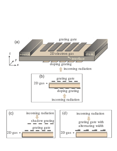
Figure 1: Design of asymmetrical grating gate structures. Optical modulation can be achieved by fabrication of doping grating from the substrate side (a) [see (b) for side view] or shadow grating from the gate side (c). Also one can use grating gate that has alternating width and alternating transparency (d).

The theory of the rachet effect neglecting plasmonic effects was developed in Refs. rachet1, ; rachet2, ; rachet4, . It predicts the Drude peak at zero frequency of the radiation and otherwise a monotonic smooth dependence of $\boldsymbol{j}$ on $\omega$ in agreement with numerical simulations Popov13 .

In this work, we demonstrate that excitation of plasmonic resonances can dramatically increase the rectified dc current. We describe the plasmonic-enhanced ratchet effect in the frame of the hydrodynamic model and obtain the analytical expression for the dc current. We demonstrate the existence of the sharp plasmonic resonances in the dependence $\boldsymbol{j}(\omega).$ The dependencies $j_{x}(\omega)$ and $j_{y}(\omega)$ turn out to be different. Remarkably, in the high-mobility structures the component $j_{y}(\omega)$ which is perpendicular to the modulation axis might be much larger than $j_{x}.$ The maximal value of the ratio $j_{y}/j_{x}$ is achieved in the vicinity of the plasmonic resonances and is proportional to the quality factor of the structure. Another intriguing property is the dependence of $j_{y}$ on the helicity of the polarization. For a single FET, the helicity-dependent response was measured Ganichev and explained theoretically Romanov by assuming a special type of the boundary conditions. The dependence of the $dc$ current on the helicity in the grating-gate periodic structures was also predicted in Refs. rachet4, ; Golub, within the approximation that ignores plasmonic effects. We will demonstrate that the helicity-dependent part of the response is also dramatically enhanced by the plasmonic effects.

We consider the electron liquid in 2D channel in the external field (2) of general polarization:

$${e_{x}}={E_{0x}}\cos{\omega}t,~{}~{}{e_{y}}={E_{0y}}\cos\left({{\omega}t+\theta}\right)$$ (3)

The case $|E_{0x}|=|E_{0y}|$, $\theta=\pm\pi/2$ corresponds to the circular polarization. For $E_{0y}=0$ the wave is linear polarized along the $x-$direction. In the absence of perturbations ($V=0,~{}\boldsymbol{E}=0$), the 2D electron concentration $N=N_{0}$ is controlled by the gate-to-channel voltage $U_{g}:$

$$N_{0}=\frac{{CU_{g}}}{e},$$ (4)

where $C=\varepsilon/4\pi d$ is the gate-to-channel capacitance per unit area, $\varepsilon$ is the dielectric constant, $d$ is the spacer distance, and $e>0$ is the absolute value of the electron charge. For smooth perturbations with $qd\ll 1$ equation (4) is also valid and relates local concentration in the channel $N=N(x,t)$ with the local gate-to-channel swing. The total electric field in the channel is given by the sum of external field of radiation, static built-in field, and electrostatic field arising due to the density perturbation: $\boldsymbol{E}_{tot}=\boldsymbol{E}-\nabla V+(e/C)\nabla N.$

The quasiclassical dynamics of electrons in the channel obeys kinetic equation:

$$\frac{\partial f}{\partial t}+\mathbf{v}{\nabla}f+\left[\boldsymbol{a}-\frac{e^{2}}{mC}{\nabla}N\right]\frac{\partial f}{\partial\mathbf{v}}={\rm St}f,$$ (5)

where $\boldsymbol{a}=-\frac{e}{m}\big{(}\boldsymbol{E}-{\nabla}V\big{)},$ and ${\rm St}f$ is the collision integral including scattering off impurities and phonons as well as electron-electron scattering. We will study electron liquid within the hydrodynamic approximation assuming the following hierarchy of the scattering times: $\tau_{ee}\ll\tau\ll\tau_{ph},$ where $\tau_{ee},\tau$ and $\tau_{ph}$ are the electron-electron, impurities and electron-phonon scattering times, respectively. These inequalities allows one to search a solution as a Fermi-Dirac function in the moving frame $f=1\left/\left[e^{m(\mathbf{v}-\boldsymbol{v})^{2}/2T-\mu/T}+1\right].\right.$ This function depends on the local hydrodynamic parameters: velocity $\boldsymbol{v}=\boldsymbol{v}(\mathbf{r},t),$ chemical potential $\mu=\mu(\mathbf{r},t),$ and temperature $T=T(\mathbf{r},t).$ In what follows we set $\mu\gg T.$ This yields $N\approx\nu\mu,$ where $\nu=m/\pi\hbar^{2}$ is the density of states. Having in mind that the electron-electron collisions conserve the particle number, momentum and energy, we multiply Eq. (5) by $1,$ $m\mathbf{v}$ and $m\mathbf{v}^{2}/2$ and integrate over momenta, thus obtaining the system of coupled equations for hydrodynamic parameters:

$$\frac{{\partial N}}{{\partial t}}+\frac{\partial}{{\partial x}}\left({N\boldsymbol{v}}\right)=0,$$ (6)

$$\frac{{\partial\boldsymbol{v}}}{{\partial t}}+(\boldsymbol{v}{\nabla})\boldsymbol{v}+\frac{\boldsymbol{v}}{\tau}=\boldsymbol{a}-\frac{{{e^{2}}}}{{mC}}{\nabla}N-\frac{{\nabla}W}{mN},$$ (7)

$${\cal C}\left[\frac{\partial T}{\partial t}+{\rm div}({T\boldsymbol{v}})\right]=N\left(\frac{T_{0}-T}{\tau_{ph}}+\frac{mv^{2}}{\tau}\right),$$ (8)

where $W=\int d\epsilon{\nu\epsilon}[e^{(\epsilon-\mu)/T}+1]^{-1}\approx{N^{2}}/{2\nu}+{\nu T^{2}\pi^{2}}/{6}$ is the system energy per unit area in the moving frame, $T_{0}$ is the lattice temperature and ${\cal C}=\nu T\pi^{2}/3$ is the heat capacity of the 2D degenerate electrons. In above, we implicitly assumed that $\tau$ is energy independent, which is the case for the impurity potential modeled by short-range disorder.

Equation (8) is coupled to Eqs. (7) and (6) by the thermoelectrical force $\pi^{2}\nu{\nabla}T^{2}/6mN=\pi^{2}T{\nabla}T/3m\mu,$ whose contribution is suppressed in the highly degenerate electron gas. Let us estimate this force in the lowest order in $T/\mu.$ To this end, we neglect l.h.s. of Eq. (8) (which is small compared to its r.h.s. due to the same parameter $T/\mu$), thus arriving to a balance equation between Joule heating and phonon cooling: $mv^{2}/\tau=(T-T_{0})/\tau_{ph}.$ Hence, the thermoelectrical force becomes $(\pi^{2}T\tau_{ph}/3\mu\tau)\nabla v^{2}.$ Comparing this force with the term $(\boldsymbol{v}\nabla)\boldsymbol{v},$ we conclude that the former is negligible provided that $\mu/T\gg\tau_{ph}/\tau.$ Assuming that this inequality is fulfilled, we are left with the system of the hydrodynamic equations for velocity and concentration:

$$\frac{{\partial n}}{{\partial t}}+\frac{\partial v_{x}}{\partial x}=-\frac{\partial(nv_{x})}{\partial x},$$ (9)

$$\frac{\partial v_{x}}{\partial t}+\frac{v_{x}}{\tau}+s^{2}\frac{\partial n}{\partial x}=a_{x}-v_{x}\frac{\partial v_{x}}{\partial x},$$ (10)

$$\frac{{\partial{v_{y}}}}{{\partial t}}+\frac{v_{y}}{\tau}=a_{y}-v_{x}\frac{\partial{v_{y}}}{\partial x},$$ (11)

where $n=(N-N_{0})/N_{0}$ and $s=\sqrt{\frac{N_{0}}{m}\left(\frac{e^{2}}{C}+\frac{1}{\nu}\right)}$ is the plasma wave velocity.

The r.h.s. of Eqs. (9), (10), and (11) includes perturbation $\boldsymbol{a}$ as well as nonlinear terms. Assuming that $\boldsymbol{a}$ is small, one can search a solution as a perturbation series over $\boldsymbol{a}:$ $n=n^{(0,1)}+n^{(1,0)}+\ldots,\hskip 8.53581pt\boldsymbol{v}=\boldsymbol{v}^{(0,1)}+\boldsymbol{v}^{(1,0)}+\ldots$ Here the two indices denote the order of smallness with regard to $\boldsymbol{e}$ and $V_{0},$ respectively. The nonzero dc current $\boldsymbol{j}=-eN_{0}{\big{\langle}{(1+n)\boldsymbol{v}}\big{\rangle}_{t,x}},$ appears in the third order with respect to $\boldsymbol{a}$ (second order in $\boldsymbol{e}$ and first order in $V_{0}$): $\boldsymbol{j}\approx\boldsymbol{j}^{(2,1)}$ (here $\langle\ldots\rangle_{t,x}$ stands for time and space averaging comment1 ). Importantly, Eqs. (9) and (10) can be solved independently from the decoupled Eq. (11) [the latter can be solved after the solution of Eqs. (9) and (10) is found]. The details of calculations are presented in the Supplementary material. Here we estimate one of the terms contributing to the $j_{x}^{(2,1)}$ in order to clarify the key points of derivation.

The static potential (1) leads to density modulation $n^{(0,1)}\propto V_{0}\cos(qx).$ The homogeneous part of the field (2) does not affect concentration but leads to the Drude peak in the velocity: $v_{x}^{(1,0)}\propto E_{0x}[e^{i\omega t}(i\omega+1/\tau)^{-1}+h.c.]$ (we omit here inhomogeneous contribution). Substituting these equations into nonlinear term $\partial\left[n^{(0,1)}v_{x}^{(1,0)}\right]/\partial x$ in the r.h.s. of Eq. (9), and solving Eqs. (9) and (10) we find that velocity in the order (1,1) exhibits plasmonic resonances as well as the Drude peak: $v_{x}^{(1,1)}\propto E_{0x}V_{0}\cos(qx)\times\left[e^{i\omega t}(i\omega+1/\tau)^{-1}(\omega^{2}-\omega_{q}^{2}-i\omega/\tau)^{-1}+h.c.\right].$ Here $\omega_{q}=sq$ is the plasma wave frequency. In turn, nonhomogeneous part of the field (2) also excites the plasmonic resonances, thus leading to density correction $n^{(1,0)}\propto E_{0x}h_{x}\sin(qx+\varphi)\left[e^{i\omega t}(\omega^{2}-\omega_{q}^{2}-i\omega/\tau)^{-1}+h.c.\right].$ Combining these equations, we find that there exists non-vanishing correction to the dc current in the order (2,1):

$$j_{x}^{(2,1)}\propto\left\langle n^{(10)}v_{x}^{(1,1)}\right\rangle_{t,x}\propto\frac{\tau}{1+\omega^{2}\tau^{2}}\frac{\sin\varphi}{(\omega^{2}-\omega_{q}^{2})^{2}+\omega^{2}/\tau^{2}}.$$

A more detailed calculations presented in Supplementary material yield:

$$j_{x}=j_{0x}\frac{2\omega_{q}^{5}\tau}{(1+\omega^{2}\tau^{2})[(\omega^{2}-\omega_{q}^{2})^{2}+\omega^{2}/\tau^{2}]},$$ (12)

$$j_{y}=j_{0y}\frac{\omega_{q}^{3}[(\omega^{2}-\omega_{q}^{2})\tau\cos\theta+\omega\sin\theta]}{(\omega^{2}-\omega_{q}^{2})^{2}+\omega^{2}/\tau^{2}}.$$ (13)

Here $j_{0x}=e^{4}V_{0}N_{0}E_{0x}^{2}h_{x}\sin\varphi/(4m^{3}s^{3}\omega_{q}^{2})$ and $j_{0y}=-e^{4}V_{0}N_{0}E_{0x}E_{0y}h_{y}\sin\varphi/(4m^{3}s^{3}\omega_{q}^{2})$ are frequency- and disorder-independent currents that are proportional to asymmetry factor $\sin\varphi$ and are sensitive to the polarization of the radiation. We note that the finite value of $j_{y}$ implies that electric circuit is closed in $y$ direction. For disconnected circuit, the voltage would develop instead, which is analogous to the Hall voltage and thus can depend on geometry of the system.

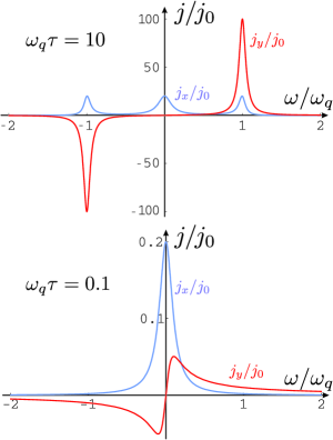
Figure 2: Frequency dependence of current components in the resonant (upper panel, $\omega_{q}\tau=10$) and non-resonant (lower panel, $\omega_{q}\tau=0.1$) cases for circular polarization ($\theta=\pi/2,~{}E_{0x}=-E_{0y},~{}h_{x}=h_{y},~{}j_{0x}=j_{0y}=j_{0}.$)

As seen from Eqs. (12) and (13), there are two different regimes depending on the plasmonic quality factor $\omega_{q}\tau.$ For $\omega_{q}\tau\gg 1,$ the response is peaked both at $\omega=0$ and at $\omega\simeq\omega_{q}$ within the frequency window $\sim 1/\tau.$ In the vicinity of the plasmonic resonance $\omega\simeq\omega_{q},$ one can simplify Eqs. (12) and (13):

$$j_{x}\approx j_{0x}\frac{2\omega_{q}\tau}{1+4(\omega-\omega_{q})^{2}\tau^{2}}$$ (14)

$$j_{y}\approx j_{0y}\frac{\omega_{q}^{2}\tau^{2}[\sin\theta+2(\omega-\omega_{q})\tau\cos\theta]}{1+4(\omega-\omega_{q})^{2}\tau^{2}}.$$ (15)

In the opposite non-resonant case, $\omega_{q}\tau\ll 1,$ we find

$$j_{x}\approx\frac{2\omega_{q}\tau j_{0x}}{1+\omega^{2}\tau_{M}^{2}},~{}j_{y}\approx\frac{\omega_{q}\tau(\omega\tau_{M}\sin\theta-\cos\theta)j_{0y}}{1+\omega^{2}\tau_{M}^{2}}$$

where the width of the response, ${1}/{\tau_{M}}=\omega_{q}^{2}\tau,$ is determined by the inverse time of the charge spreading at the distance $\sim q^{-1}$ (Maxwell relaxation time).

In the resonant regime $\boldsymbol{j}$ is much larger than in the non-resonant case (due to the largeness of $\omega_{q}\tau$) and shows sharp resonant dependence on $\omega$ (see Fig. 2). Hence, excitation of plasmons leads to a dramatic enhancement of the rachet effect. Note that for $\theta=\pm\pi/2,$ $j_{y}$ changes its sign with the sign of $\theta$, i.e. at switching between right and left circular polarizations. Thus, our results predict strong helicity effect - the circular polarization of the incident light determines the direction of $j_{y}.$ Remarkably, for clean systems transverse component of the current, $j_{y}^{max}/j_{0y}\sim(\omega_{q}\tau)j_{x}^{max}/j_{0x},$ might be much larger than the longitudinal one provided that $\omega_{q}\tau$ is sufficiently large. It worth also stressing that for $\theta=\pm\pi/2$ transverse current remain finite in the dissipationless limit $\tau\to\infty:$ $j_{y}\to\pm j_{0y}\omega_{q}^{3}\omega/(\omega^{2}-\omega_{q}^{2})^{2}.$

To conclude, we predicted a dramatic enhancement of the ratchet effect due to the excitation of plasmonic resonances. We identified a helicity-dependent contribution to the ratchet current and found that this contribution increases with decreasing the static disorder and saturates in the limit $\tau\to\infty.$ We also demonstrated that the non-resonant ratchet current is sharply peaked at zero frequency within the inverse Maxwell relaxation time.

We thank S. Ganichev, L. Golub, A. Muraviev, and V. Popov for stimulating discussions. The work has been supported by grant FP7-PEOPLE-2013-IRSES of the EU network Internom and by RFBR.

I Supplementary material

In this Supplementary material, we present a rigorous derivation of dc current in the channel based on iteration of Eqs. (9), (10), and (11) with respect to $\boldsymbol{a}$. Non zero response appears in the order (2,1) and can be written as a sum of terms arising at different steps of iterations:

$$\boldsymbol{j}^{(2,1)}=-eN_{0}\big{\langle}n^{(2,0)}\boldsymbol{v}^{(0,1)}+n^{(1,1)}\boldsymbol{v}^{(1,0)}$$ (16)

$$+n^{(1,0)}\boldsymbol{v}^{(1,1)}+n^{(0,1)}\boldsymbol{v}^{(2,0)}+\boldsymbol{v}^{(2,1)}\big{\rangle}_{t,x}.$$

Next, we calculate all terms entering Eq. (16) separately for $j_{x}$ and $j_{y}.$

I.1 Calculation of $j_{x}.$

We start with calculation of the $x-$component of the current. In the orders (0,1) and (1,0) the nonlinear terms in the r.h.s. of Eqs. (9) and (10) are absent, so that we are left with linear equations, whose solution yields $n^{(0,1)},n^{(1,0)},v_{x}^{(0,1)},v_{x}^{(0,1)}.$ Next, we substitute this solution into nonlinear terms and make the next iteration which yields the terms of the orders (2,0), (1,1), and (0,2) (all terms in the second order in $\boldsymbol{a}$). The solution in the order $(i,j)$ can be simply written in the matrix form in the $(Q,\Omega)$ domain

$$\left(\begin{array}[]{c}n\\ v_{x}\end{array}\right)_{Q,\Omega}^{(i,j)}=\frac{i}{\Omega^{2}-\omega_{Q}^{2}+i\Omega/\tau}\left[\begin{array}[]{cc}\Omega+i/\tau&Q\\ s^{2}Q&\Omega\\ \end{array}\right]\left(\begin{array}[]{c}J_{n}\\ J_{x}\end{array}\right)_{Q,\Omega}^{(i,j)}.$$ (17)

Here $\omega_{Q}=sQ$ is the plasma wave frequency and $J_{n}^{(i,j)}$ and $J_{x}^{(i,j)}$ are the r.h.s. of Eqs. (9) and (10), respectively, in the order $ij.$ Due to nonlinearity of the problem, frequency $\Omega$ and the wave vector $Q$ arising at each step of iterations are discrete and given by harmonics of the $\omega$ and $q,$ respectively: $\Omega=M\omega,~{}Q=Kq,$ where $M$ and $K$ are integer numbers. For $\Omega=\pm\omega,~{}Q=\pm q,$ and $\omega\approx\omega_{q}$ there appear a plasmonic resonances in the ratchet response.

In the order (0,1), we have: $J_{n}^{(0,1)}=0,~{}J_{x}^{(0,1)}=-(eqV_{0}/m)\sin(qx).$ Using Eq. (17) (with $\Omega=0$ and $Q=\pm q$), we find

$$v_{x}^{(0,1)}=0,$$ (18)

$$n^{(0,1)}=\frac{eV_{0}}{ms^{2}}\cos(qx).$$ (19)

Next, we find $J_{n}^{(1,0)}=0,~{}J_{x}^{(1,0)}=-(eE_{0x}/m)\cos(\omega t)[1+h_{x}\cos(qx)],$ so that there are two types of terms: with $\Omega=\pm\omega,~{}Q=0$ and with $\Omega=\pm\omega,~{}Q=\pm q.$ From Eq. (17) we get

$$n^{(1,0)}=\frac{eE_{0x}h_{x}q\sin(qx+\varphi)e^{i\omega t}}{2m(\omega^{2}-\omega_{q}^{2}-i\omega/\tau)}+h.c.,$$ (20)

$$v_{x}^{(1,0)}=-\frac{eE_{0x}h_{x}\omega\cos(qx+\varphi)e^{i\omega t}}{2im(\omega^{2}-\omega_{q}^{2}-i\omega/\tau)}$$ (21)

$$-\frac{eE_{0x}e^{i\omega t}}{2m(i\omega+1/\tau)}+~{}h.c..$$

Next, we substitute obtained solutions in the nonlinear terms and find

$$J^{(1,1)}_{x}=-\frac{\partial\big{[}v_{x}^{(1,0)}v_{x}^{(0,1)}\big{]}}{\partial x}=0,$$ (22)

$$J_{n}^{(1,1)}=-\frac{\partial\left[n^{(1,0)}v^{(0,1)}+n^{(0,1)}v^{(1,0)}\right]}{\partial x}$$ (23)

$$=\frac{e^{2}E_{0x}V_{0}q\sin(qx)e^{i\omega t}}{2m^{2}s^{2}(i\omega+1/\tau)}+h.c.+\ldots.$$

Here and in what follows $(\ldots)$ stands for terms oscillating in space with the wave vector $2q.$ We skip them since their contribution drops out from $j_{x}^{(2,1)}$ after space averaging. Substituting Eqs. (22) and (23) in Eq. (17), we find

$$n^{(1,1)}=-\frac{e^{2}E_{0x}V_{0}q\sin(qx)e^{i\omega t}}{2m^{2}s^{2}(\omega^{2}-\omega_{q}^{2}-i\omega/\tau)}+h.c.+\ldots,$$ (24)

$$v_{x}^{(1,1)}=\frac{e^{2}E_{0x}V_{0}q^{2}\cos(qx)e^{i\omega t}}{2m^{2}(i\omega+1/\tau)(\omega^{2}-\omega_{q}^{2}-i\omega/\tau)}$$ (25)

$$+h.c.+\ldots.$$

As seen from Eq. (16) what is left to be done is the calculation of $v_{x}^{(2,1)}$ and $v_{x}^{(2,0)}.$

Let us first demonstrate that

$$\left\langle v_{x}^{(2,1)}\right\rangle_{t,x}=0.$$ (26)

To this end, we notice that all terms entering Eq. (10) except $v_{x}/\tau$ can be written as derivatives over $t$ or $x.$ Hence, averaging this equation over time and distance we find that $\left\langle v_{x}\right\rangle_{t,x}=0,$ and, consequently, $\left\langle v_{x}^{(i,j)}\right\rangle_{t,x}=0$ for any $i$ and $j.$

In order to find $\left\langle v_{x}^{(2,0)}n^{(0,1)}\right\rangle_{t,x},$ we first write Eq. (9) in the order (2,0),

$$\frac{\partial n^{(2,0)}}{\partial t}+\frac{\partial v_{x}^{(2,0)}}{\partial x}=-\frac{\partial\left[n^{(1,0)}v_{x}^{(0,1)}+n^{(0,1)}v_{x}^{(1,0)}\right]}{\partial x}.$$ (27)

Then, we average this equation over time. Since $v_{x}^{(0,1)}=0,$ we get

$$\frac{\partial\left[v^{(2,0)}_{x}+n^{(1,0)}v_{x}^{(1,0)}\right]}{\partial x}=0.$$ (28)

Hence

$$\left\langle v_{x}^{(2,0)}\right\rangle_{t}=-\left\langle n^{(1,0)}v_{x}^{(1,0)}\right\rangle_{t}+\xi(t),$$ (29)

where $\xi(t)$ is function of $t$ only. Having in mind that $n^{(0,1)}$ depends on $x$ only and $\left\langle n^{(0,1)}\right\rangle_{x}=0,$ we get

$$\left\langle v_{x}^{(2,0)}n^{(0,1)}\right\rangle_{t,x}=-\left\langle n^{(0,1)}n^{(1,0)}v_{x}^{(1,0)}\right\rangle_{t,x}.$$ (30)

Now, we can calculate $j_{x}.$ Using Eqs. (21) and (24) we find $\left\langle v_{x}^{(1,0)}n^{(1,1)}\right\rangle_{t,x}=0.$ Since $v_{x}^{(1,0)}=0,$ we conclude that only two terms contribute to $j_{x}:$

$$j_{x}^{(2,1)}=-eN_{0}\left\langle n^{(1,0)}v^{(1,1)}_{x}-n^{(0,1)}n^{(1,0)}v^{(1,0)}_{x}\right\rangle_{t,x}.$$ (31)

Substituting Eqs. (19), (20), (21), and (25) into Eq. (31) and averaging over $t$ and $x,$ we find that both terms in Eq. (31) yield equal contributions. The total current $j_{x}\approx j^{(2,1)}_{x}$ is given by Eq. (12) of the main text.

I.2 Calculation of $j_{y}$

In this subsection, we find transversal component of current solving Eq. (11) by iterations with respect to small $\boldsymbol{a}.$ In the order $(i,j)$ solution in $(Q,\Omega)$ space reads

$$v_{y}^{(i,j)}(Q,\Omega)=\frac{J_{y}^{(i,j)}(Q,\Omega)}{1/\tau-i\Omega},$$ (32)

where $J_{y}^{(i,j)}(x,t)$ is the r.h.s. of Eq. (11).

In the first order with respect to $\boldsymbol{a}$ we find

$$J_{y}^{(0,1)}(x,t)=0,$$ (33)

$$J_{y}^{(1,0)}(x,t)=a_{y}=-\frac{eE_{0y}}{m}\cos(\omega t+\theta)$$ (34)

$$\times[1+h_{y}\cos(qx+\varphi)].$$

Using Eq. (32) we get

$$v^{(0,1)}_{y}=0,$$ (35)

$$v_{y}^{(1,0)}=\frac{eE_{0y}[1+h_{y}\cos(qx+\varphi)]e^{i(\omega t+\theta)}}{2m(i\omega+1/\tau)}$$ (36)

$$+~{}h.c.$$

Next, we consider terms of the second order with respect to $\boldsymbol{a}$. In the order (1,1) we get

$$J_{y}^{(1,1)}=-v_{x}^{(1,0)}\frac{\partial v_{y}^{(0,1)}}{\partial x}-v_{x}^{(0,1)}\frac{\partial v_{y}^{(1,0)}}{\partial x}=0,$$ (37)

so that

$$v_{y}^{(1,1)}=0$$ (38)

Having in mind Eqs. (35) and (38) we find from Eq. (16)

$${j}_{y}^{(2,1)}=-eN_{0}\big{\langle}n^{(1,1)}v^{(1,0)}_{y}+n^{(0,1)}{v}_{y}^{(2,0)}+{v}_{y}^{(2,1)}\big{\rangle}_{t,x}.$$ (39)

From Eqs. (24) and (36) we obtain

$$\big{\langle}n^{(1,1)}v^{(1,0)}_{y}\big{\rangle}_{t,x}=-\frac{e^{3}E_{0x}E_{0y}h_{y}V_{0}q\sin\varphi}{4m^{3}s^{2}(\omega^{2}+1/\tau^{2})}$$ (40)

$$\times\frac{[(\omega_{q}^{2}/\tau)\cos\theta+\omega(\omega_{q}^{2}-\omega^{2}-1/\tau^{2})\sin\theta]}{(\omega^{2}-\omega_{q}^{2})^{2}+\omega^{2}/\tau^{2}}.$$

As follows from Eq. (19), $n^{(0,1)}$ does not depend on $t.$ Thus, while calculating contribution of the second term in Eq. (39) we can first average in time ${v}_{y}^{(2,0)}.$ Averaging over time Eq. (11), we find in the order (2,0)

$$\big{\langle}v_{y}^{(2,0)}\big{\rangle}_{t}=\tau\left\langle v_{x}^{(1,0)}\frac{\partial v_{y}^{(1,0)}}{\partial x}\right\rangle_{t}.$$ (41)

Hence,

$$\left\langle n^{(0,1)}{v}_{y}^{(2,0)}\right\rangle_{t,x}=\tau\left\langle n^{(0,1)}v_{x}^{(1,0)}\frac{\partial v_{y}^{(1,0)}}{\partial x}\right\rangle_{t,x}$$ (42)

$$=\frac{e^{3}E_{0x}E_{0y}h_{y}V_{0}q\tau\sin\varphi\cos\theta}{4m^{3}s^{2}(\omega^{2}+1/\tau^{2})}.$$

Here we used Eqs. (19), (21), and (36).

Analogously, averaging over time and distance Eq. (11) in the order (2,1), and using Eqs. (25) and (36), we get

$$\left\langle v_{y}^{(2,1)}\right\rangle_{t,x}=\tau\left\langle v_{x}^{(1,1)}\frac{\partial v_{y}^{(1,0)}}{\partial x}\right\rangle_{t,x}$$ (43)

$$=-\frac{e^{3}E_{0x}E_{0y}h_{y}V_{0}q^{3}\tau\sin\varphi}{4m^{3}(\omega^{2}+1/\tau^{2})}$$

$$\times\frac{[(\omega^{2}-\omega_{q}^{2})\cos\theta+(\omega/\tau)\sin\theta]}{(\omega^{2}-\omega_{q}^{2})^{2}+\omega^{2}/\tau^{2}}.$$

Finally, substituting Eqs. (40), (42), and (43) into Eq. (39), we find that $j_{y}\approx j_{y}^{(2,1)}$ is given by Eq. (13) of the main text.

References

• (1) M. I. Dyakonov and M. S. Shur, Phys. Rev. Lett. 71, 2465 (1993).
• (2) M. I. Dyakonov and M. S. Shur, IEEE Trans. on Elec. Dev. 43, 380 (1996).
• (3) W. J. Stillman and M. S. Shur, J. of Nanoelectronics and Optoelectronics. 2, 209 (2007).
• (4) D. Veksler, F. Teppe, A. P. Dmitriev, V. Yu. Kachorovskii, W. Knap, M. S. Shur, Phys. Rev. B 73, 125328 (2006).
• (5) G. C. Dyer, G. R. Aizin, S. Preu, N. Q. Vinh, S. J. Allen, J. L. Reno, and E. A. Shaner, Phys. Rev. Lett. 109, 126803 (2012)
• (6) G. R. Aizin, G. C. Dyer, Phys. Rev. B 86 235316 (2012).
• (7) V. Yu. Kachorovskii and M. S. Shur, Appl. Phys. Lett. 100, 232108 (2012)
• (8) Gregory C. Dyer, Gregory R. Aizin, S. James Allen, Albert D. Grine, Don Bethke, John L. Reno, and Eric A. Shaner Nature Photonics 7, 925 (2013).
• (9) Lin Wang, Xiaoshuang Chen, Weida Hu1, Anqi Yu, and Wei Lu, Appl. Phys. Lett. 102, 243507 (2013).
• (10) X. G. Peralta, S. J. Allen, M. C. Wanke, N. E. Harff, J. A. Simmons, M. P. Lilly, J. L. Reno, P. J. Burke, and J. P. Eisenstein, Appl. Phys. Lett. 81, 1627 (2002).
• (11) E. A. Shaner, Mark Lee, M. C. Wanke, A. D. Grine, J. L. Reno, and S. J. Allen, Appl. Phys. Lett. 87, 193507 (2005).
• (12) E. A. Shaner, M. C. Wanke, A. D. Grine, S. K. Lyo, J. L. Reno, and S. J. Allen, Appl. Phys. Lett. 90, 181127 (2007).
• (13) A. V. Muravjov, D. B. Veksler, V. V. Popov, O. V. Polischuk, N. Pala, X. Hu, R. Gaska, H. Saxena, R. E. Peale, and M. S. Shur Appl. Phys. Lett. 96, 042105 (2010).
• (14) G. C. Dyer, S. Preu, G. R. Aizin, J. Mikalopas, A. D. Grine, J. L. Reno, J. M. Hensley, N. Q. Vinh, A. C. Gossard, M. S. Sherwin, S. J. Allen, and E. A. Shaner , Appl. Phys. Lett., 100, 083506 (2012).
• (15) G. R. Aizin, V. V. Popov, and O. V. Polischuk Appl. Phys. Lett. 89, 143512 (2006).
• (16) G. R. Aizin, D. V. Fateev, G. M. Tsymbalov, and V. V. Popov Appl. Phys. Lett. 91, 163507 (2007).
• (17) T. V. Teperik, F. J. Garci’a de Abajo, V. V. Popov, and M. S. Shur Appl. Phys. Lett. 90, 251910 (2007).
• (18) V. V. Popov, D. V. Fateev, T. Otsuji, Y. M. Meziani, D. Coquillat, and W. Knap, Appl. Phys. Lett. 99, 243504 (2011).
• (19) Y. M. Meziani, H. Handa, W. Knap, T. Otsuji, E. Sano, V. V. Popov, G. M. Tsymbalov, D. Coquillat, and F. Teppe Appl. Phys. Lett. 92, 201108 (2008).
• (20) T. Otsuji, Y. M. Meziani, T. Nishimura, T. Suemitsu, W. Knap, E. Sano, T. Asano, and V. V. Popov, J. Phys.: Condens. Matter bf 20, 384206 (2008).
• (21) M. Büttiker, Z. Phys. B 68, 161 (1987).
• (22) Ya. M. Blanter and M. Büttiker, Phys. Rev. Lett. 81, 4040 (1998).
• (23) A.M. Song, P. Omling, L. Samuelson, W. Seifert, I. Shorubalko, and H. Zirath, Appl. Phys. Lett. 79, 1357 (2001).
• (24) E.M. Höhberger, A. Lorke, W. Wegscheider, and M. Bichler, Appl. Phys. Lett. 78, 2905 (2001).
• (25) P. Reimann, Phys. Rep. 361, 57 (2002).
• (26) H. Linke (ed.), Ratchets and brownian motors: Basics, experiments and applications, special issue, Appl. Phys. A: Mater. Sci. Process. A 75, 167 (2002).
• (27) P. Olbrich, E. L. Ivchenko, R. Ravash, T. Feil, S. D. Danilov, J. Allerdings, D. Weiss, D. Schuh, W. Wegscheider, and S. D. Ganichev, Phys. Rev. Lett. 103, 090603 (2009).
• (28) Yu.Yu. Kiselev and L.E. Golub, Phys. Rev. B 84, 235440 (2011).
• (29) P. Olbrich, J. Karch, E. L. Ivchenko, J. Kamann, B. März, M. Fehrenbacher, D. Weiss, and S. D. Ganichev, Phys. Rev. B 83, 165320 (2011).
• (30) E.L. Ivchenko and S. D. Ganichev, Pisma v ZheTF 93, 752 (2011) [JETP Lett. 93, 673 (2011)].
• (31) V.V. Popov, D.V. Fateev, T. Otsuji, Y.M. Meziani, D. Coquillat, and W. Knap, Appl. Phys. Lett. 99, 243504 (2011).
• (32) B. Sothmann, R. Sánchez, A. N. Jordan, and M. Büttiker, Phys. Rev. B 85, 205301 (2012).
• (33) A. V. Nalitov, L. E. Golub, E. L. Ivchenko, Phys. Rev. B 86, 115301 (2012).
• (34) V. V. Popov, Appl. Phys. Lett. 102, 253504 (2013).
• (35) Note that for realistic systems the density and field perturabtions can not be described by simple harmonic fucnctions and involve infinite number of harmonics (see Ref. ivchenko ). Also, the field amplitude $\boldsymbol{e}$ is much smaller than the amplitude of the external field due to the screening by the gate electrodes. However, the simplified model based on Eq. (1) and (2) with phenomenological parameters $V_{0},$ $E_{0x},$ and $E_{0y}$ captures the key physics of the problem and is sufficient for clarifying the basic concept of the plasmon-enhanced ratchet.
• (36) E. L. Ivchenko, M. I. Petrov Physics of the Solid State September 2014, 56, 1833 (2014) [Fizika Tverdogo Tela, 2014, 56, 1772 (2014)].
• (37) C. Drexler, N. Dyakonova, P. Olbrich, J. Karch, M. Schafberger, K. Karpierz, Y. Mityagin, M. B. Lifshits, F. Teppe, O. Klimenko, Y. M. Meziani, W. Knap, and S. D. Ganichev, Journal of Applied Physics 111, 124504 (2012).
• (38) K. S. Romanov and M. I. Dyakonov, Appl. Phys. Lett. 102, 153502 (2013).
• (39) In fact, averaged in time $\boldsymbol{j}$ does not depend on $x,$ so that it is sufficient to make averaging over $t$ only. However, calculations are strongly simplified if we make also $x$-averaging in all contributing terms.