Evidence of Economic Regularities and Disparities of Italian Regions From Aggregated Tax Income Size Data

Abstract

This paper discusses the size distribution, - in economic terms - of the Italian municipalities over the period 2007-2011. Yearly data are rather well fitted by a modified Lavalette law, while Zipf-Mandelbrot-Pareto law seems to fail in this doing. The analysis is performed either at a national as well as at a local (regional and provincial) level. Deviations are discussed as originating in so called king and vice-roy effects. Results confirm that Italy is shared among very different regional realities. The case of Lazio is puzzling.

Keywords: City size distribution, Lavalette law, Zipf’s law, rank-size rule, Italian cities, aggregated tax income.

1 Introduction

The analysis of the ranking of elements belonging to a specific set under a predefined criterion leads to the identification of a best fit curve, through the rank-size theory (Jefferson 1939, Zipf 1949, Beckmann 1958, Gabaix 1999a, Gabaix 1999b) and its applications.
This paper deals with the rank-size rule for the entire set of municipalities in Italy (IT, hereafter) for each year of the quinquennium 2007-2011. The size is here given by the contribution (so called Aggregated Tax Income, thereby denoted hereafter as ATI) that each city has given to the Italian GDP (data are expressed in Euros); cities are yearly ranked according to the value of their related ATI. Data are official, and have been provided directly from the Research Center of the Italian Minister of Economic Affairs.
For our investigation, several different directions are followed:

• the possible law describing the relationship between ranking and ATI is explored. In particular, we show that Zipf, Zipf-Mandlebrot and power laws fail in this doing. A more convincing answer is provided by the Lavalette function (Popescu, 2003),

  $$y(rank)=K\;\Big{(}\frac{N\cdot rank}{N-rank+1}\Big{)}^{-\chi}\;\equiv\;\kappa\;\Big{(}\frac{rank}{N-rank+1}\Big{)}^{-\chi}$$ (1.1)

  which has been introduced in 1996 by the biophysicist Daniel Lavalette. Such an analysis is performed not only at the country, but also at the regional and at the provincial level;

• the distribution of the ATI at the regional level is lengthily explored. In doing so, several cities are shown to exhibit a prominent role in determining a relevant percentage of the national GDP (the so-called king and king plus vice-roy effects, see Section 4.2 for the details).

In particular, point 1. supports that sometimes data city sizes do not have pure Zipf-type (i.e. a pure power law) links with the corresponding ranks. However, evidence is here shown that some particular subsets of cities may be well described by a statistically appealing Zipf-Mandelbrot law (this is the paradigmatic case of Lazio, an IT region), - a set of considerations postponed for an Appendix (App. A) in order to let a relatively ordered line of thought guiding the reader in the following sections, - without being distracted by the main aims. For the contextualization of these results in the literature, see Section 2.
Also point 2. is in great agreement with an improvement of the best-fit results when some specific subsets of data are considered. In this case, king and king plus vice-roy effects can be appreciated by observing, on displayed plots, that removing the first and sometimes the first set of ranked cities, respectively, leads (not always, but remarkably often) to a more statistically convincing Lavalette curve.
It is important to point out that, to the best of our knowledge, this is the first contribution dealing with the application of the Lavalette curve to the field of urban economics; it was invented and usually applied for bibliometrics studies.
The paper is organized as follows: Section 2 briefly reviews the literature inspiring and connected to the present research. Section 3 contains the description of the data. Section 4 is devoted to the investigation of the whole IT, with the assessment of some rank-size rule fits on yearly basis. This section contains also the ATI ranking analysis at a regional level, with all the plots of the 2-parameter Lavalette functions and the detection of the outliers. Section 5 collects and discusses the findings. The last section (Sect. 6) concludes and offer suggestions for further research lines. Appendix A describes the Lazio case, while Figures and Tables pertaining to the regional data analysis are collected in Appendix B.

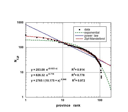
Figure 1: Log-log plot of the number $N_{c,p}$ of cities (8092) per provinces (110), ranked by decreasing order of ”importance”; showing fits by a power law, an exponential and a Zipf-Mandlebrot function with the corresponding correlation coefficient.

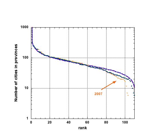
Figure 2: Semi-log- plot of the number, $N_{c,p}$, of cities in a province ranked by decreasing order of ”importance”, for the studied 5 years (2007-2011); the best mere 2-parameter Lavalette function fit, Eq. (1.1), is shown for year 2011 only for better visibility ($R^{2}$=0.985); the 2007 year, with 5 less provinces, is also emphasized; all best 2-parameter Lavalette function fits are found in Table 2.

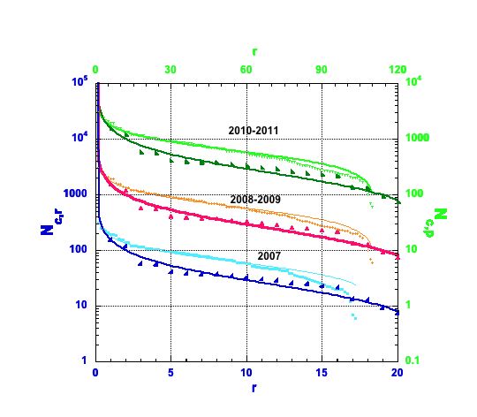
Figure 3: Semi-log- plot of the number of cities in a province, $N_{c,p}$, and in a region, $N_{c,r}$, ranked by decreasing order of ”importance”, for various years; the 2007, 2008-2009 and 2010-2011 data are displaced by an obvious factor for better readability; the best mere 2-parameter Lavalette function, Eq. (1.1), fit is shown for $N_{c,p}$, with $N_{p}$ =110; a forced 2-parameter Lavalette function with $N_{r}=24$ (instead of $N_{r}=20$) is used for $N_{c,r}$ to improve $R^{2}$; all best 2-parameter Lavalette function fits are found in Table 2.

2 Review of the literature

In the context of New Economic Geography (NEG), - introduced by Krugman (1991) and surveyed in Ottaviano and Puga (1998), Fujita et al. (1999), Neary (2001), Baldwin et al. (2003) and Fujita and Mori (2005), spatial patterns based on geographical agglomerations and dispersions of economic quantities play a fundamental role. In discussing the features of the geographical entities, city population size distribution represents one of the most debated themes, and there is a wide literature discussing on how the rank-size rule can be properly described.
In this respect, power law and Pareto distribution with coefficient one (the so-called Zipf’s law, introduced in Zipf (1935, 1949), stating that a hyperbolic relationship exists between rank and size), seems to provide a rather satisfactory answer. Several studies proved empirically the validity of Zipf’s law: Rosen and Resnick (1980) analyzed data from 44 Countries, and found a clear predominance of statistical significance of Zipf’s law, with $R^{2}$ greater than 0.9 (except in one case, Thailand); in Mills and Hamilton (1994), data from US cities in 1990 has been taken to show the evidence of Zipf’s law ($R^{2}\sim 0.99$); other papers which substantially support this type of rank-size rule are Guerin-Pace (1995), Dobkins and Ioannides (2001), Song and Zhang (2002), Ioannides and Overman (2003), Gabaix and Ioannides (2004), Reed (2002), Dimitrova and Ausloos (2013) just to cite a few. Nitsch (2005) provides an exhaustive literature review up to that time. It is also worth mentioning Simon (1955), Gabaix (1999a, 1999b) and Brakman et al. (1999), who have the merit to have tried to provide an explanation of Zipf’s law. However, Gabaix (1999b) criticized Simon (1955) reasoning in saying that it is grounded on assumptions on the Pareto parameter that seem to be not empirically supported.
Recently, Dimitrova and Ausloos (2013), through the notion of the global primacy index of Sheppard (1985) indicated that Gibrat (growth) law (Gibrat, 1931), supposedly at the origin of Zipf’s law, in fact, does not hold in the case of Bulgaria cities.
Thus, in general, why the rank-size rule can be described in many cases through the Zipf’s law remains still a puzzle. This lack of a theoretical basis for this statistical results has been acknowledged by influential scientists (see Fujita et al., 1999; Fujita and Thisse, 2000).
Moreover, Zipf’s law is not a universal law at all, in the sense that some data does not support such a way to link rank and size of the cities. As an example, the above-mentioned case of Thailand in Rosen and Resnick (1980) concerns a weak correlation between data plot and Pareto fit. Peng (2010) found a Pareto coefficient of $0.84$ -not so close to one!, - when implementing a best fit of data on Chinese city sizes in 1999-2004 through Pareto distribution. Ioannides and Skouras (2013), like others, argue that Pareto law seems to stand in force only in the tail of the data distribution. Matlaba et al. (2013) provided evidence that, at least for the analyzed case of Brazilian urban areas over a spectacularly wide period (1907-2008), Zipf’s law is clearly rejected.
The failure of Zipf’s law may depend often on the way data are grouped (Giesen and Südekun, 2011). In this respect, Soo (2007) proves empirically that the size of Malaysian cities cannot be plotted according to such rank-size rule, but a suitable collection of them can do it. A list of other contributions on the inconsistency of Zipf’s law in several countries, different periods and under specific economic conditions should include Cordoba (2008), Garmestani et al. (2007) and Bosker et al. (2008). Of particular interest is also Garmestani et al. (2008), who conduct an analysis for the US at a regional level.
From the present state of the art point of view, regional agglomerations, commonly ranked in terms of population, may be also sorted out in an order dealing with the economic variables. In fact, Zipf’s law is sometimes identified also in some ”economic” way to rank. As an example, Skipper (2011) used such a rank-size relationship to detect well developed countries order through their national GDP. This result has been also achieved by Cristelli et al. (2012), who exhibited evidence of the Zipf’s law for the top fifty richest countries in the period 1900-2008. One can then conclude as McCann (2013) does, in stating that [Zipf’s law holds] irrespective of whether the regional size is measured in terms of population or GDP. This is in contrast with Nobel laureate Krugman previous statement that the rank-size rule is ”a major embarrassment for economic theory: one of the strongest statistical relationships we know, lacking any clear basis in theory.” (Krugman, 1995, p.44).
No need to say that, therefore, more data analysis can bring some information on resolving the controversy. Moreover, the investigation seems new, since there is, to our knowledge, no statistical evidence of Zipf’s law studies for the economic variables characterizing Italian cities (in the period 2007-2011).
Note that investigations of the contributions (= sizes) that local entities bring to the national GDP have been often studied. Those investigations are the main themes of so many publications that references cannot be even short listed. However, much literature has been rather concerned with convergence effects (as in L ́opez-Bazo et al., 1999) which have not been the main themes of the present investigation. Rather than searching for effects, we have been aiming at observing and quantifying structural causes.

3 Data

Data collect the disaggregated contributions at a municipal level (in IT a municipality or city is denoted as comune, - plural $comuni$) to the Italian GDP.
The data source is the Research Center of the Italian Minister of Economic Affairs, and the covered period is the quinquennium 2007-2011.
Under an administrative point of view, Italy is composed of 20 regions, more than 100 provinces and more than 8000 municipalities. Each municipality is included in one specific province, which in turns belongs to one and only one region. Several administrative laws modified the number of provinces and municipalities during the quinquennium, and also of the number of cities in each entity, but the number of regions has been constantly equal to 20 (see below the time dependence of the precise values).
Therefore, the available yearly ATI data corresponds to a different number of cities. In particular, the number of cities has been yearly evolving respectively as follows : 8101, 8094, 8094, 8092, 8092, - from 2007 till 2011.
However, scientific consistency imposes to compare identical lists. In 2011, the number of provinces and municipalities is 110 and 8092, respectively. We have considered this latest 2011 ”count” as the basic one. Therefore, we have taken into account a virtual merging of cities, in the appropriate (previous to 2011) years, according to IT administrative law statements (see also $http://www.comuni-italiani.it/regioni.html$).
In brief, several cities have thus merged into new ones, other were phagocytized. Here below are the various cases ”of interest” explaining some ”data reorganization”:

• Campolongo al Torre (UD) and Tapogliano (UD) have merged after a public consultation, held on Novembre 27th, 2007, into Campolongo Tapogliano (UD); thus 2 $\rightarrow$ 1

• LEDRO (TN) was the result of the merging (after a public consultation, held on Novembre 30th, 2008) of Bezzecca (TN), Concei (TN), Molina di Ledro (TN), Pieve di Ledro (TN), Tiarno di Sopra (TN) and Tiarno di Sotto (TN) as far as it is explained e.g. in $http://www.tuttitalia.it/trentino-alto-adige/18-concei/$; thus 6 $\rightarrow$ 1

• Comano Terme (TN) results from the merging of Bleggio Inferiore (TN) and Lomaso (TN), in force of a regional law of November 13th, 2009; thus 2 $\rightarrow$ 1

• Consiglio di Rumo (CO) and Germasino (CO) were annexed by Gravedona (CO) on May 16th, 2011 and February 10th, 2011, to form the new municipality of Gravedona ed Uniti (CO); thus 3 $\rightarrow$ 1.

To sum up: 13 $\rightarrow$ 4.
Thus, 8092 municipalities is our reference number. In short, the ATI (studied in Sect. 4 and in Sect. 4.1) of the resulting cities have been linearly adapted, as if these were preexisting before the merging or phagocytosis. A summary of the statistical characteristics for the year-dependent ATI of all Italian cities over the period 2007-2011 can be found in Table 1. Table Appendix B. Tables and Figures contains the yearly ranked top and bottom cities in Italy in the sample period.

	2007	2008	2009	2010	2011
min. (x$10^{-5}$)	3.0455	2.9914	3.0909	3.6083	3.3479
Max. (x$10^{-10}$)	4.3590	4.4360	4.4777	4.5413	4.5490
Sum (x$10^{-11}$)	6.8947	7.0427	7.0600	7.1426	7.2184
mean ($\mu$) (x$10^{-7}$)	8.5204	8.7033	8.7248	8.8267	8.9204
median ($m$) (x$10^{-7}$)	2.2875	2.3553	2.3777	2.4055	2.4601
RMS (x$10^{-8}$)	6.5629	6.6598	6.6640	6.7531	6.7701
Std. Dev. ($\sigma$) (x$10^{-8}$)	6.5078	6.6031	6.6070	6.6956	6.7115
Var. (x$10^{-17}$)	4.2351	4.3601	4.3653	4.4831	4.5044
Std. Err. (x$10^{-6}$)	7.2344	7.3404	7.3448	7.4432	7.4609
Skewness	48.685	48.855	49.266	49.414	49.490
Kurtosis	2898.7	2920.42	2978.1	2991.0	2994.7
$\mu/\sigma$	0.1309	0.1318	0.1321	0.1319	0.1329
$3(\mu-m)/\sigma$	0.2873	0.2884	0.2883	0.2878	0.2889

Table 1: Summary of (rounded) statistical characteristics for ATI of IT cities ($N=8092$) in 2007-2011.

Note that, in this time window, the data claims a number of 103 provinces in 2007, with an increase by 7 units (BT, CI, FM, MB, OG, OT, VS) thereafter, leading to 110 provinces. In this respect, it is worth noting a discrepancy between what data say and the real legislative evolution of the provinces. In fact, 4 provinces have been instituted by a regional law of 12 July 2001 in Sardinia and became operative in 2005 (CI, MB, OG, OT), while BT, FM and VS have been created on June 11th, 2004 and became operative on June 2009. However, the official data provided by the Economics Minister are here taken as scientific basis, and the number of provinces is then 103, 110, 110, 110, 110 - from 2007 till 2011.
Some (mild) effect of this $provincial$ variation is discussed below, although the emphasis of the present discussion is about the $regional$ level.

4 Regional and provincial analysis

In order to stress the regional aspect, the number of cities per regions, and also per provinces, ranked in decreasing order of ”importance” is examined, i.e. the number of cities in a region or in a province is the ”size measure”, in this section; see Figs. 1-3:

• on Fig. 1 it is seen that a mere 2-parameter decaying power law (blue) or a 2-parameter decaying exponential (green) as well as a 3-parameter Zipf-Mandelbrot function (red) are neither visually nor statistically appealing (see the $R^{2}$ value) for describing the number of cities in the provinces as function of the rank, $N_{c,p}(rank)$. Therefore, further specific investigations are needed to assess the data. These are however beyond the scope of the present paper, limiting ourselves here to fits based on only a 2-parameter function;

• in contrast, Fig. 2, a double $x$ - double $y$ plot, reports a fit of the ranking of the 110 provinces, according to the number of cities, $N_{c,p}$ by a 2-parameter Lavalette function, Eq. (1.1). It seems to be a rather good fit, to say the least, with $R^{2}=0.985$. Some deviation occurs at high rank ($r\geq 60$), but there are not many cities (less than 50) in each of these few provinces. The 5 yearly cases are hardly distinguishable from each other. Observe some different data range for 2007: recall that there are 7 provinces less in 2007 than in other subsequent years. To better distinguish the various years, Fig. 3 shows the rank size variation for $N_{c,p}$, the number of cities in each province, fitted with the appropriate 2-parameter Lavalette function.

	2007	2008	2009	2010	2011
$N_{c}$	8101	8094	8094	8092	8092
$N_{p}$	103	110	110	110	110
provinces: $N_{c,p}$
$\kappa$	62.41	61.07	61.07	61.07	61.08
$\chi$	0.369	0.371	0.371	0.371	0.371
$R^{2}$	0.973	0.985	0.985	0.985	0.985
regions: $N_{c,r}$
$\kappa$	225.97	225.56	225.56	225.77	225.77
$\chi$	0.607	0.608	0.608	0.608	0.608
$R^{2}$	0.953	0.953	0.953	0.953	0.953

Table 2: Parameters of the Lavalette function, Eq. (1.1), for the fits (see data displayed in Fig. 3) of the number of cities in regions and in provinces, for various years; the number of regions $N_{r}$ is always equal to 20; the number of provinces $N_{p}$ has changed as indicated.

	$N_{c,p}$	$N_{c,r}$
Minimum	6	74
Maximum	315	1544
Mean ($\mu$)	73.564	404.6
Median ($m$)	60	319
RMS	91.902	536.998
Std Deviation ($\sigma$)	55.338	362.253
Variance	3 062.27	131 227.52
Std Error	5.2762	81.0023
Skewness	1.7294	2.1284
Kurtosis	3.6845	3.8693
$\mu/\sigma$	1.329	1.117
$3(\mu-m)/\sigma$	0.7353	0.7089

Table 3: Summary of (rounded) statistical characteristics for the number ($N_{c}=8092$) distribution of IT cities in the various ($N_{p}=110$) provinces and regions ($N_{r}=20$) in 2011. The maximum $N_{c,p}$ value is 315 for (TO), while the minimum one is 6 for (TS); $N_{c,r}=$ 1544 (Lombardia) and 74 (Valle d’Aosta) for the regions respectively, - see Table 4.

	$N_{c,r}$
Lombardia	1544
Piemonte	1206
Veneto	581
Campania	551
Calabria	409
Sicilia	390
Lazio	378
Sardegna	377
Emilia Romagna	348
Trentino Alto Adige	333
Abruzzo	305
Toscana	287
Puglia	258
Marche	239
Liguria	235
Friuli Venezia Giulia	218
Molise	136
Basilicata	131
Umbria	92
Valle d’Aosta	74

Table 4: Number $N$ of (8092) cities (in 2011) in the (20) IT regions; such a region ranking by city number corresponds to that illustrated in Figs. 1- 3.

The best Lavalette 2-parameter fits, with Eq. (4.1) form, are found in Table 2. Some illustrative statistical characteristics of the city distributions as function of region $r$ and province $p$, $N_{c,r}$ and $N_{c,p}$ respectively, - in 2011 as an example, are also given in Table 3.

2007			2008
Altidona	(AP)	29 235 733	Altidona	(FM)	30 329 015
Andria	(BA)	565 869 043	Andria	(BT)	581 635 172
Arcore	(MI)	293 056 037	Arcore	(MB)	300 146 626
Arzana	(NU)	17 002 253	Arzana	(OG)	18 200 141

Table 5: Examples of 4 cities, and their ATI, - observe quite different orders of magnitude, having a province change but remaining in the same region, at their years change. Data are expressed in Euros.

2007 (PU) - Marche		2008 (RN) - Emilia Romagna
Casteldelci	3 221 694	Casteldelci	3 171 730
Maiolo	7 395 158	Maiolo	7 596 247
Novafeltria	78 547 921	Novafeltria	80 178 021
Pennabilli	28 814 429	Pennabilli	29 100 286
San Leo	27 411 857	San Leo	28 792 554
St Agata Feltria	24 563 898	St Agata Feltria	24 046 727
Talamello	11 371 705	Talamello	11 808 818

Table 6: The 7 cities (see text) having had a province change and also a region change; their ATI is given at their years change. As written in the Table, PU (the province of Pesaro and Urbino) is in the Marche region, while RN (province of Rimini) is in the Emilia Romagna region. Data are expressed in Euros.

4.1 Regional disparities

In this section, in view of respecting ”scientific constraints” which impose to tie geography and economy along New Economy Geography ideas (Krugman 1995), we consider every IT region (made of provinces and cities). We search whether the ATI of the cities in each region obey simple hierarchical relationships, - like a 2-parameter free Lavalette function.
First of all, it is worth to point out that 228 municipalities have changed from a province to another one, but nevertheless remained in the same region (see Table 5 for a few examples), while 7 municipalities have changed from a province to another one, -in fact also changing from a region to another (these 7 cases are given in Table 6).
Therefore, one can summarize the number of cities belonging to a region as in Table 4. This corresponds to Figs. 2-3, in fact. The display of the distribution characteristics of these cities for the 110 provinces obviously requests 110 Tables (or Figures). They are not given here, but any province case can be available from the authors, - upon request.
The following points have to be taken into account before display and analysis:

• the plot illustrating the relationship between $N_{c,r}$ (and $N_{c,p}$) and their respective rank is year dependent;

• the same comment applies for ATI_c,r (and ATI_c,p), in obvious notations: they are year dependent;

• finally, it is worth noting that the plots of the relationship between the ATI_c, i.e. aggregated to the whole country, and their rank is year dependent, but not due to the change in the number of cities. This simplifies the analysis.

A technical point is needed here. In order to optimize the fit procedure, i.e., also in order to have a $\kappa$ value characterized by a few digits, the Lavalette function, Eq. (1.1) has been thereafter opportunely rescaled by a $10^{6}$ factor ($\sim y(N/2)$) also dropping the $N$ factor of the rank $r$:

$$y(rank)=\hat{\kappa}\;10^{6}\Big{(}\frac{rank}{N-rank+1}\Big{)}^{-\chi}.$$ (4.1)

4.2 ATI distributions in IT regions. Time, ”King”, and ”Vice-Roy Effects”

Before displaying and discussing the evolution of the various regions from the ATI of their member cities point of view, a practical remark is in order. It is often found, and has been found in the present study, that an upsurge occurs at low ranks. In other words, the best (simplest, like power law or exponential or Zipf, as those considered in Sect.4) fits are impaired because the low rank data can be much above (sometimes an order of magnitude) whatever function is used in the appropriate fit, resulting in an outlier for $r\rightarrow 1$. This, observed a long time ago by Jefferson (1989), has been called a king effect by Laherrere and Sornette (1998), when examining the population size of French cities (or rather agglomerations). For example, the number of inhabitants in Paris is much bigger than the (theoretical) value resulting from the best (estimated, stretched exponential) plot. In presence of only one outlier, the king (K) effect is identified. When an occurrence of several outliers is observed, then there is king plus vice-roy effect (KVR).
Such ATI (or city) outliers are observed in almost all regions and provinces, as shown below.
For convincing the reader, let two cases be shown, as examples:

• consider the 384 largest IT cities, in terms of population size, for the whole Italy, as ranked by decreasing order, and compare such a size-rank relationship to a power law; as indicated in Fig. 4, it is obvious that there are 6 ”outliers” (in order from the biggest: Roma, Milano, Napoli, Torino, Palermo, Genova);

• a similar situation occurs when examining ATI values, rather than population sizes: consider the 384 ”richest” IT cities, in terms of ATI size, for the whole Italy, as ranked by decreasing order, and compare such a size-rank relationship to a power law; see Fig. 5, it is obvious that there are 8 ”outliers” (in order from the biggest: Roma (RM), Milano (MI), Torino (TO), Genova (GE), Napoli (NA), Bologna (BO), Palermo (PA), Firenze (FI)). For completeness, let it be known that from the ATI ranking point of view, the top 12 IT cities have never changed their ranking, i.e. these 8 plus Venezia (VE), Verona (VR), Bari (BA), and Padova (PD).

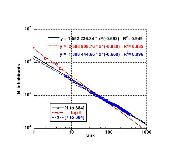
Figure 4: The 384 largest IT cities ranked by decreasing order according to their population size with corresponding power law fits as indicated, pointing to 6 outliers.

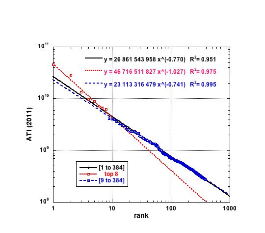
Figure 5: The 384 ”richest” IT cities ranked by decreasing order according to their ATI with corresponding power law fits as indicated, pointing to 8 outliers.

Observe that $6\neq 8$, see that cities are differently ranked, and what city is added to the ATI outliers with respect to the population size ones.
Although the demonstration in such figures is made through a log-log plot with power law fits, the same effects occur when using exponential or Lavalette function fits on semi-log plots. Similar situations occur for the regional and provincial level though not necessarily so well marked due to the smaller number of data points and their size value, - surely in the province cases. Nevertheless, in order to obtain some reasonable estimates of the empirical relations over a large range of data, it seems obviously necessary to take into account such a king effect, - in almost all the data, we have examined. Moreover, because such king effects, as seen in Figs. 4 - 5, in fact truly occur over a rank interval $\geq 1$, it has been necessary to consider king plus vice-roy effect, accounting for more than 1 outlier, - as made more precise in the figure captions.
When a flattening of the data occurs at low rank, a so called queen, or often a queen plus harem, effect appears (Ausloos 2013); the ”problem” is different from the KVR effect; a Zipf-Mandelbrot-Pareto law is of course a more appropriate description, in such cases. None has been found to occur in the present study.
Nevertheless, a special case has to be pointed out at once here. Although, it is shown that the Lavalette law usually well represent the ATI data, a 3-parameter Zipf-Mandlebrot-Pareto law fits unexpectedly well the Lazio region data, - as long as the rank is $2\leq r\leq 101$. The illustration, statistical analysis and some specific discussion are postponed to Appendix A, for this special region. This finding confirms a classical statement, i.e. the soundness of the Zipf’s law can hold for a subset of a collection of data, but does not necessarily hold for the entire set. This is in accord with the empirical evidence registered in previous studies (see Section 2, for references to the literature on this).
Results are displayed in Figs. 9-29, whose captions are rather detailed. The parameters of the best fits are reported in Tables 7-8. A discussion is presented in Section 5.

5 Results and discussion

This section fixes and discusses the results of the investigation.
First, a rank-size rule, on the basis of the number of cities per province, has been searched through Zipf-Mandelbrot-Pareto, power and exponential laws. It statistically failed. However, the rank-size rule for the cities in Lazio region can be well described by those curves. This fact confirms the finding of some researchers that a subset of a sample can be well represented by Zipf’s law while the whole sample may fail in this doing (we address the reader to the discussion in Section 2 and Appendix A). Should it be necessary to the reader to recall that the Lazio region contains Roma, the capital city of Italy? and can thus be expected to present a superking effect.
The 2-parameter Lavalette law seems to suitably fit, - with a high level of $R^{2}$ and/or visual soundness between curve and data, the rank-size rule for Italy cities under different perspective and size-detection criteria. Specifically: $(i)$ number of cities per region; $(ii)$ number of cities per province. The occurring deviations for low rank, more evident in case $(ii)$, are due to the (KVR-like) outliers and to the creation of 7 new provinces during the observed period.
In exploring the regional cases, several facts emerge.
As for what concerns the low-rank elements in the Zipf’s law case (see e.g. Gabaix, 2009), the role of the outliers at high rank is rather huge in the Lavalette case. For several regions, a strong king or king plus vice-roy effect may destroy the statistical consistence of the mere 2-parameter Lavalette curve in plotting the data. The $R^{2}$ is not necessarily small, the visual appeal of the fit is weak: this is due in such fits to the importance taken by the low rank (thus high ATI values) of a few cities. In such cases, removing the outliers can lead to a more convincing fit (paradigmatic cases are Aosta Valley, Basilicata, Campania, Friuli Venezia Giulia, Liguria, Lombardia, Molise, Puglia, Sicilia, and Trentino Alto Adige). Other cases provide a substantial indifference in removing the outliers, with neither an appreciable improvement of the visual appeal of the graphs nor of the $R^{2}$ (many cases are not displayed, for shortening the paper), like Abruzzo, Marche, Sardegna, Umbria and Veneto. A few cases give rise to questions, but with some answer: in fact, in several cases the removal of the outliers implies unexpected not much better results from a $R^{2}$, point of view, but in presence of a better visualization of the fit; this is the case of Friuli Venezia Giulia. A slightly less appealing visualization of the fit with a slightly smaller $R^{2}$ occurs also for Emilia Romagna. Valle d’Aosta is the region where the KVR-effect must be removed for a fine fit.
Sometimes, there is some surprise, thus no real ”answer”: Trentino Alto Adige, Molise and Sicilia are found to have a large number of vice-roys. Also, fits to the Marche data are rather insensitive to a KVR effect removal, although the $R^{2}$ is at first, for the raw data, not very high.
Finally, Lazio seems to be not properly described by a 2-parameter Lavalette function, but rather through exponential, ZMP, and power laws, as already mentioned (see the discussion above).
In view of the above, it seems that there is some evidence that the KVR effects are not due to scale factors, but are intrinsic to the regularities and discrepancies, since the KVR effect occurs in most cases, - found in quite different size systems.

6 Conclusions

This paper provides a statistical analysis of the Italian municipalities for the period 2007-2011, ranked by their ATI values. It is proven that while ZMP, exponential and power laws are not statistically appealing in describing the size-rank rule, a 2-parameter Lavalette function is. To the best of our knowledge, this is the first time that such typology of function is employed in urban studies.
Data also confirm that IT is a unique entity, but with different regional realities. Several cities play a prominent role in determining the Italian GDP; they are detected within the regions through the king and king plus vice-roy effects. We have observed that there is some evidence that the KVR effects are not due to scale factors, but are intrinsic to the economic regularities and discrepancies.
A few cases are puzzling, and suggest some further investigation of this theme. Thus, a refinement of the analysis through the introduction of a 3-parameter Lavalette function or a modified version of it is in order. In particular, the second aspect suggests to work in the direction of a theoretical improvement of the current literature on the laws describing rank-size rules.

Appendix A. The Lazio case

It has been indicated in the main text that a 3-parameter Zipf-Mandelbrot-Pareto law fits unexpectedly well the Lazio region ATI data, - as long as the rank is $3\leq r\leq 101$, much better than a Lavalette function; see Fig. 6 for the 2011 case, on a log-log plot (and Fig. 17 for all 5 years on a semi-log plot). Another mere exponential fit (not shown) to the whole data, except for the king (Roma) and vice-roy (Latina) data points also indicates a strong cut-off at $r\geq 100$.
For illustration and completeness, indicating that other possible fits were investigated, Figs. 7-8 show a fit to a power law with exponential cut-off at high rank, and a comparison of such a fit with a Zipf-Mandelbrot-Pareto law, respectively, on a log-log plot, for the ATI 2011 year, - as an example, when either the Roma point or the Roma and Latina data points are not considered.

Figure 6: Log-log plot of the ranked 2011 ATI Lazio cities -$r$ represents here the rank-, showing fits by a Lavalette function (red line) and a Zipf-Mandelbrot-Pareto function (blue line), for $3\leq r\leq 101$, i.e. when the king (Roma) and vice-roy (Latina) data points (large black square dots) are excluded from the fits.

Figure 7: Log-log plot of the ($r$) ranked 2011 ATI Lazio cities, showing fits by a power law with an exponential cut-off, when either (red line) the king (Roma) or (blue line) king plus vice-roy (Latina) data points (large black square dots) are excluded from the fits; the regression coefficients are given.

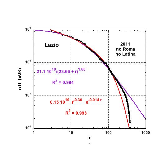
Figure 8: Log-log plot of the ranked 2011 ATI Lazio cities, showing fits by a power law with an exponential cut-off (red line) at high rank ($r$) compared to a ZMP law (violet line), with their corresponding regression coefficient, when either the king (Roma) and vice-roy (Latina) data points are excluded from the fits.

Appendix B. Tables and Figures

This Appendix contains

• the figures, Figs. 9-29, relative to the ranking of cities according to their ATI, and best fits by a Lavalette function, sometimes for the raw data, sometimes taking into account a K effect of a KVR effect. It is here mentioned, once and for all, that the data 2011 data is $not$ rescaled, but all ATI data scales for the other years are systematically reduced for the display by a factor 10^m, where $m$ is the difference between 2011 and the year of interest;

• the parameters of the best fits to a Lavalette function of the raw data, in Tables 7-8; a column indicates how many KVR cities can be considered (and removed) in order to optimize the fits reported in the corresponding figures;

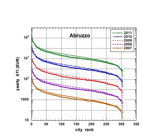
Figure 9: Abruzzo, a regional case of ATI distributions; $N$=305 cities are ranked accordingly; with 2-parameter Lavalette fits; neither king plus vice roy effect nor king effect is observed.

Figure 10: Ranked ATI yearly values for Aosta Valley, a regional case with (obviously) king plus vice-roy effect (Aosta and Sarre); $N$=74; with 2-parameter Lavalette fits.

Figure 11: Fit of a 2-parameter free Lavalette function to ranked ATI yearly values for the $N=131$ ranked cities, when removing Potenza and Matera, as king and vice-roy cities.

Figure 12: Calabria city yearly ATI ranking distribution 2-parameter Lavalette fits; $N$=409, but removing a remarkable king effect as Reggio Calabria for the fit. Nevertheless, note the departure from a ”good looking fit” at high rank in the most recent years.

Figure 13: Campania, city yearly ATI ranking distribution and 2-parameter Lavalette fits ($N$=451), but after removing a remarkable king plus vice-roy effect (Napoli and Salerno).

Figure 14: Ranked ATI yearly values for Emilia Romagna cities with 2-parameter Lavalette fits. N.B. $N=341$ in 2007, but $N=348$ otherwise. Moreover, there is no need for optimizing the fit in considering Bologna as inducing a king effect. Nevertheless, note the departure from a ”good looking fit” at high rank in the most recent years.

Figure 15: Friuli Venezia Giulia city ATI distribution: $N$=219 in 2007 $\rightarrow$ 218 thereafter and 2-parameter Lavalette fits, but admitting a king and vice-roy (Trieste and Udine) effect, - as observed when such a fit on the full data is attempted.

Figure 16: ATI yearly distribution for Lazio ($N$=378) cities; 2-parameter Lavalette fits, after removal of king plus vice-roy effect (Rome and Latina).

Figure 17: Lazio, $N$=378 cities; 2-parameter Lavalette fits. Comparison between raw data and removal of king plus vice-roy effect (Rome and Latina) is amazing, - in this worse encountered case.

Figure 18: Ranked ATI yearly values for Liguria ($N$=235) cities; 2-parameter Lavalette fits, after removal of king effect (Genova).

Figure 19: Ranked city ATI yearly values for Lombardia region: 2010 and 2011 for $N$=1546 cities; 2007, 2008, and 2009 for $N$=1544 cities; fits with the 2-parameter Lavalette function, after removing the Milano king effect data point.

Figure 20: Marche: $N$=246 cities in 2007 and $N$=239 thereafter; fits of ATI yearly raw data with the 2-parameter Lavalette function. No king or king plus vice-roy effect is observed in this region.

Figure 21: Molise $N$=136 cities ranked according to their yearly ATI, with the 2-parameter Lavalette function fits. Remarkably a king (Campobasso) with 3 vice-roys (Termoli, Isernia, Venafro), i.e. N-4 data points are used, effect here is very meaningful; the corresponding fits on the whole $N$=136 data are indicated by continuous lines.

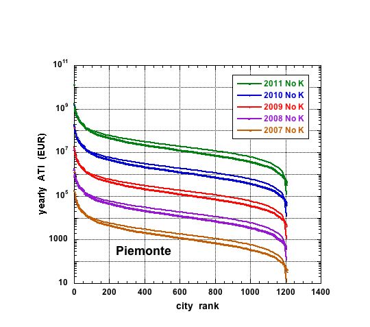
Figure 22: Piemonte $N$=1206 cities yearly ATI with 2-parameter Lavalette function fits. Remarkably a king (Torino) must be withdrawn for a realistic fit improvement

Figure 23: Yearly ATI ranked data of Puglia $N$=258 cities fitted with the 2-parameter Lavalette function, taking into account a king (Bari) and a vice-roy (Taranto) effect, - for very fine fits

Figure 24: Yearly ATI ranked data of Sardegna, $N$=377 cities, with 2-parameter Lavalette function for fitting. Considering any king or king plus vice-roy effect gives not much improvement of the fit.

Figure 25: Ranked ATI yearly value distributions for Sicilia cities: $N$=390 and subsequent 2-parameter Lavalette fits, but admitting a king and two vice-roys (Palermo, Catania and Messina) effect.

Figure 26: Toscana city yearly ranked ATI distribution: $N$=287 and subsequent 2-parameter Lavalette fits, but admitting a king (Firenze) effect.

Figure 27: Trentino-Alto Adige: a regional case comparing ATI values through 2-parameter Lavalette fits in 2008-2011 for $N$=333 cities, and in 2007 for $N$=339 cities, taking into account in both cases a king (Trento) and three vice-roys (Bolzano, Merano, and Rovereto), thus removing the corresponding data points before fits.

Figure 28: Distribution of Umbria $N$=287 cities ranked according to their yearly ATI, - data fitted with the 2-parameter Lavalette function. No need to search for king or king plus vice-roy effect, but note the remarkable hump at $r$=60 with departure from the fit at high $r$.

Figure 29: Distribution of Veneto $N$=581 cities ranked according to their yearly ATI, - data fitted with the 2-parameter Lavalette function. No need to search for king or king plus vice-roy effect.

Region		2007	2008	2009	2010	2011	KVR	Fig.
Abruzzo	$\hat{\kappa}$	15.43	15.725	15.89	16.19	16.81		9
Abruzzo	$\chi$	0.814	0.805	0.809	0.809	0.805
Abruzzo	$R^{2}$	0.986	0.981	0.986	0.986	0.986	0
Aosta Valley	$\hat{\kappa}$	0.589	0.624	0.635	0.665	0.698		10
Aosta Valley	$\chi$	1.574	1.566	1.566	1.558	1.546
Aosta Valley	$R^{2}$	0.911	0.909	0.909	0.910	0.908	2
Basilicata	$\hat{\kappa}$	7.223	7.782	7.888	7.866	7.782		11
Basilicata	$\chi$	0.978	0.966	0.966	0.969	0.966
Basilicata	$R^{2}$	0.923	0.920	0.920	0.917	0.920	2
Calabria	$\hat{\kappa}$	7.195	7.471	7.834	7.947	8.103		12
Calabria	$\chi$	0.915	0.913	0.909	0.907	0.902
Calabria	$R^{2}$	0.993	0.994	0.994	0.994	0.994	1
Campania	$\hat{\kappa}$	0.134	0.151	0.166	0.169	0.151		13
Campania	$\chi$	1.756	1.738	1.724	1.722	1.738
Campania	$R^{2}$	0.945	0.943	0.942	0.942	0.943	2
Em.Romagna(*)	$\hat{\kappa}$	60.77	61.60	61.32	62.49	63.81		14
Em.Romagna(*)	$\chi$	0.810	0.807	0.807	0.804	0.800
Em.Romagna(*)	$R^{2}$	0.977	0.977	0.977	0.976	0.976	1
FriuliVG(**)	$\hat{\kappa}$	8.662	8.61	0.8219	8.313	8.547		15
FriuliVG(**)	$\chi$	1.093	1.099	1.110	1.108	1.102
FriuliVG(**)	$R^{2}$	0.980	0.979	0.979	0.979	0.978	2
Lazio	$\hat{\kappa}$	!	!	!	!	!		16
Lazio	$\chi$	!	!	!	!	!
Lazio	$R^{2}$	!	!	!	!	!	2	(17)
Liguria	$\hat{\kappa}$	0.028	0.030	0.030	0.031	0.033		18
Liguria	$\chi$	2.327	2.321	2.321	2.317	2.307
Liguria	$R^{2}$	0.984	0.984	0.984	0.984	0.983	1
Lombardia(***)	$\hat{\kappa}$	0.002	0.002	0.002	0.002	0.002		19
Lombardia(***)	$\chi$	2.233	2.231	2.228	2.243	2.253
Lombardia(***)	$R^{2}$	0.956	0.955	0.954	0.954	0.954	1

Table 7: (I) Parameter values of the ATI data fits with the adapted 2-parameter Lavalette function, Eq. (4.1), every considered year: $\hat{\kappa}*10^{6}*[r/(N-r+1)]^{-\chi}$; with $\hat{\kappa}$= 1 and $\chi$ = 1 as initial iteration conditions; $N$ depends on the year and the region: it is usually given by the value in Table 4, except for (*) $N=341$ (2007) $\rightarrow$ 348 (2008-11); (**) $N=219$ (2007) $\rightarrow$ 218 (2008-11); (***) $N=1546$ (2007-09) $\rightarrow$ 1544 (2010-11). Lazio is so meaningless, see Fig. 16, that values are not shown (see the discussion in the text). KVR column stands for how many king effect and king plus vice-roys effect are taken into account in the mentioned figure to improve $R^{2}$$\rightarrow 0.99$.

Region		2007	2008	2009	2010	2011	KVR	Fig
Marche(#)	$\hat{\kappa}$	37.05	38.63	38.22	38.99	40.29		20
Marche(#)	$\chi$	0.696	0.695	0.697	0.695	0.689
Marche(#)	$R^{2}$	0.964	0.963	0.965	0.964	0.962	0
Molise	$\hat{\kappa}$	3.525	3.672	3.539	3.552	3.605		21
Molise	$\chi$	1.049	1.046	1.054	1.053	1.053
Molise	$R^{2}$	0.979	0.978	0.979	0.978	0.978	3
Piemonte	$\hat{\kappa}$	0.005	0.005	0.006	0.006	0.007		22
Piemonte	$\chi$	2.092	2.084	2.062	2.065	2.047
Piemonte	$R^{2}$	0.952	0.952	0.951	0.950	0.949	1
Puglia	$\hat{\kappa}$	34.33	36.34	37.30	37.87	39.29		23
Puglia	$\chi$	0.844	0.837	0.833	0.832	0.824
Puglia	$R^{2}$	0.985	0.985	0.985	0.985	0.985	2
Sardegna	$\hat{\kappa}$	8.141	8.741	9.048	9.032	9.155		24
Sardegna	$\chi$	0.953	0.945	0.940	0.942	0.939
Sardegna	$R^{2}$	0.986	0.987	0.987	0.987	0.988	0
Sicilia	$\hat{\kappa}$	10.26	10.73	11.20	11.18	11.71		25
Sicilia	$\chi$	1.077	1.072	1.067	1.068	1.058
Sicilia	$R^{2}$	0.983	0.982	0.982	0.982	0.982	3
Toscana	$\hat{\kappa}$	47.39	48.47	49.33	49.78	50.16		26
Toscana	$\chi$	0.844	0.842	0.839	0.839	0.839
Toscana	$R^{2}$	0.981	0.981	0.980	0.981	0.980	1
Tr.-A.Adige(##)	$\hat{\kappa}$	8.681	9.304	9.573	9.982	9.304		27
Tr.A.Adige(##)	$\chi$	0.936	0.930	0.929	0.924	0.930
Tr.-A.Adige(##)	$R^{2}$	0.922	0.923	0.924	0.924	0.923	4
Umbria	$\hat{\kappa}$	27.99	28.92	29.44	29.59	30.33		28
Umbria	$\chi$	0.975	0.973	0.970	0.971	0.964
Umbria	$R^{2}$	0.986	0.986	0.986	0.987	0.987	0
Veneto	$\hat{\kappa}$	35.88	36.79	36.50	37.35	38.45		29
Veneto	$\chi$	0.770	0.767	0.768	0.765	0.760
Veneto	$R^{2}$	0.895	0.895	0.896	0.895	0.897	0

Table 8: (II) Parameter values of the ATI data fits with the adapted 2-parameter Lavalette function, Eq. (4.1), every considered year: $\hat{\kappa}*10^{6}*[r/(N-r+1)]^{-\chi}$; with $\hat{\kappa}$= 1 and $\chi$ = 1 as initial iteration conditions; $N$ depends on the year and the region: it is usually given by the value in Table 4, except for : (^#) N= 246 in 2007 $\rightarrow$ 239 thereafter; (^##) $N=336$ (2007) $\rightarrow$ 333 (2008-11). KVR column stands for how many king and king plus vice-roys are taken into account in the mentioned figure to improve $R^{2}$$\rightarrow 0.99$.

Top and bottom modifications of ranked IT cities according to their ATI, during the 5 years of interest.
Recall that the top 12 cities do not change their rank; see text
rank	2007	2008	2009	2010	2011
13	Trieste	Trieste	Trieste	Trieste	Parma
14	Parma	Parma	Parma	Parma	Trieste
15	Brescia	Brescia	Brescia	Modena	Brescia
16	Modena	Modena	Modena	Brescia	Modena
17	Catania	Catania	Catania	Catania	Catania
18	Messina	Reggio Emilia	Messina	Messina	Reggio Emilia
19	Reggio Emilia	Messina	Reggio Emilia	Reggio Emilia	Messina
20	Prato	Prato	Prato	Prato	Prato
21	Monza	Monza	Cagliari	Perugia	Cagliari
22	Perugia	Perugia	Perugia	Cagliari	Perugia
23	Cagliari	Cagliari	Ravenna	Ravenna	Ravenna
24	Bergamo	Ravenna	Monza	Monza	Monza
8080	Baradili	Falmenta	Morterone	Falmenta	Ribordone
8081	Mnt.Leone Rocca Doria	Morterone	Torresina	Morterone	Ingria
8082	Castelmagno	Mnt.Lapiano	Canosio	Carapelle Calvisio	Torresina
8083	Torresina	Canosio	Cervatto	Cervatto	Cervatto
8084	Salza Di Pinerolo	Elva	Salza Di Pinerolo	Cavargna	Falmenta
8085	Moncenisio	Torresina	Cavargna	Ingria	Cavargna
8086	Elva	Carapelle Calvisio	Carapelle Calvisio	Torresina	Elva
8087	Cervatto	Moncenisio	Elva	Elva	Castelmagno
8088	Menarola	Cervatto	Cursolo-Orasso	Cursolo-Orasso	Menarola
8089	Canosio	Menarola	Menarola	Menarola	Cursolo-Orasso
8090	Pedesina	Pedesina	Moncenisio	Val Rezzo	Val Rezzo
8091	Cursolo-Orasso	Cursolo-Orasso	Pedesina	Moncenisio	Pedesina
8092	Val Rezzo	Val Rezzo	Val Rezzo	Pedesina	Moncenisio

References

- [1] Ausloos, M., 2013. A scientometrics law about co-authors and their ranking. The co-author core, Scientometrics 95, 895-909.
- [2] Baldwin, R., Forslid, R., Martin, P., Ottaviano, G., Nicoud, F., 2003. Economic geography and public policy. Princeton, NJ: Princeton University Press.
- [3] Beckmann, M., 1958. City Hierarchies and the Distribution of City Size, Economic Development and Cultural Change 6, 243-248.
- [4] Bosker, M., Brakman, S., Garretsen, H., Schramm, M., 2008. A century of shocks: the evolution of the German city size distribution 1925-1999, Regional Science and Urban Economics 38(4), 330-347.
- [5] Brakman, G., Garretsen, H., van Marrewijk, C., van den Berg, M., 1999. The Return of Zipf: Towards a Further Understanding of the Rank-Size Distribution, Journal of Regional Science 39(1), 182-213.
- [6] Cordoba, J.-C., 2008. On the distribution of city sizes, Journal of Urban Economics 63(1), 177-197.
- [7] Cristelli, M., Batty, M., Pietronero, L., 2012. There is more than a power law in Zipf, Scientific reports 2, 812.
- [8] Dimitrova, Z., Ausloos, M., 2013. Primacy analysis of the system of Bulgarian cities, arXiv preprint : .
- [9] Dobkins, L.H., Ioannides, Y.M., 2001. Spatial interactions among U.S. cities: 1900-1990, Regional Science and Urban Economics 31(6), 701-731.
- [10] Eurostat office at: .
- [11] Fujita, M., Krugman, P., Venables, A.J., 1999. The Spatial Economics: Cities, Regions, and International Trade, The MIT Press, Cambridge, MA.
- [12] Fujita, M., Mori. T., 2005. Frontiers of the New Economic Geography, Papers in Regional Science 84(3), 377-405.
- [13] Fujita, M., Thisse, J.-F., 2000. The formation of economic agglomerations: Old problems and new perspectives, in: Huriot, J.M., Thisse, J.-F. (Eds.), Economics of Cities: Theoretical Perspectives, Cambridge Univ. Press, Cambridge, UK.
- [14] Gabaix, X., 1999a. Zipf law for Cities: An Explanation, Quarterly Journal of Economics 114(3), 739-767.
- [15] Gabaix, X., 1999b. Zipf law and the Growth of Cities American Economic Review 89(2), 129-132.
- [16] Gabaix, X., Ioannides, Y.M., 2004. The Evolution of City Size Distributions, in: Henderson, J.V., Thisse, J.-F. (Eds.), Handbook of Regional and Urban Economics, Vol. 4, Amsterdam, Elsevier.
- [17] Garmestani, A.S., Allen, C.R., Gallagher, C.M., Mittelstaedt, J.D., 2007. Departures from Gibrat’s Law, Discontinuities and City Size Distributions, Urban Studies 44(10), 1997-2007.
- [18] Garmestani, A.S., Allen, C.R., Gallagher, C.M., 2008. Power laws, discontinuities and regional city size distributions, Journal of Economic Behavior and Organization 68, 209-216.
- [19] Gibrat, R., 1931. Les in égalités économiques: Applications aux inégalités des richesses, à la concentration des entreprises, aux populations des villes, aux statistiques des familles, etc., d’une loi nouvelle, la loi de l’effet proportionnel. Paris: Sirey.
- [20] Giesen, K., Südekum, J., 2011. Zipf law for cities in the regions and the country, Journal of Economic Geography 11(4), 667-686.
- [21] Guérin-Pace, F., 1995. Rank-size distribution and the process of urban growth, Urban Studies 32(3), 551-562.
- [22] Ioannides, Y.M., Overman, H.G., 2003. Zipf s law for cities: an empirical examination, Regional Science and Urban Economics 33(2), 127-137.
- [23] Ioannides, Y.M., Skouras, S., 2013. US city size distribution: robustly Pareto, but only in the tail, Journal of Urban Economics 73(1), 18-29.
- [24] Italian regions and municipalities at:
- [25] Jefferson, M., 1939. The Law of Primate City, Geographical Review 29(2), 226-232.
- [26] Krugman, P., 1991. Geography and Trade, Cambridge MA: The MIT Press.
- [27] Krugman, P., 1995. Development, Geography, and Economic Theory, Cambridge MA: The MIT Press.
- [28] Laherrere, J., Sornette, D., 1998. Stretched exponential distributions in nature and economy fat tails with characteristic scales, European Physics Journal B 2(4), 525-539.
- [29] Levenberg, K., 1944. A method for the solution of certain problems in least squares, Quarterly Applied Mathematics 2, 164-168.
- [30] López-Bazo, E., Vayá, E., Mora, A.J., Surinach, J., 1999. Regional economic dynamics and convergence in the European Union, The Annals of Regional Science 33(3), 343-370.
- [31] Lourakis, M.I.A., 2011. A Brief Description of the Levenberg-Marquardt Algorithm Implemented by levmar, Foundation of Research and Technology 4, 1-6.
- [32] Marquardt, D.W., 1963. An Algorithm for Least-Squares Estimation of Nonlinear Parameters, Journal of the Society for Industrial and Applied Mathematics 11(2), 431-441.
- [33] Matlaba, V. J., Holmes, M. J., McCann, P., Poot, J., 2013. A century of the evolution of the urban system in Brazil, Review of Urban and Regional Development Studies 25(3), 129-151.
- [34] McCann, P., 2013. Modern Urban and Regional Economics, 2nd Edition. Oxford University Press.
- [35] Mills, E. S., Hamilton, B.W., 1994. Urban Economics, Prentice Hall.
- [36] Neary, J.P., 2001. Of Hype and Hyperbolas: Introducing the New Economic Geography, Journal of Economic Literature 39(2), 536-561.
- [37] Nitsch, V., 2005. Zipf zipped, Journal of Urban Economics 57(11), 86-100.
- [38] Ottaviano, G., Puga, D., 1998. Agglomeration in the global economy: A survey of the new economic geography , The World Economy 21(6), 707-731.
- [39] Peng, G., 2010. Zipf’s law for Chinese cities: Rolling sample regressions, Physica A: Statistical Mechanics and its Applications 389(18), 3804-3813.
- [40] Popescu, I., 2003. On a Zipf’s law extension to impact factors. Glottometrics 6, 83-93.
- [41] Reed, W.J., 2002. On the Rank-Size Distribution for Human Settlements, Journal of Regional Science 42(1), 1-17.
- [42] Rosen, K.T., Resnick, M., 1980. The size distribution of cities: an examination of the Pareto law and primacy, Journal of Urban Economics 8(2), 165-186.
- [43] Sheppard, E., 1985. Urban System Population Dynamics: Incorporating Nonlinearities, Geographical Analysis 17(1), 47-73.
- [44] Simon, H., 1955. On a Class of Skew Distribution Functions, Biometrika 42(314), 425-440.
- [45] Skipper, R.K., 2011. Zipf’s Law and Its Correlation to the GDP of Nations, McNair Scholars Undergraduate Research Journal 3, 217-226.
- [46] Song, S., Zhang, K.H., 2002. Urbanisation and city size distribution in China, Urban Studies 39(12), 2317-2327.
- [47] Soo, K.T., 2007. Zipf law and urban growth in Malaysia, Urban Studies 44(1), 1-14.
- [48] Zipf, G.K., 1935. The Psychobiology of Language, Houghton-Mifflin.
- [49] Zipf, G., 1949. Human Behavior and the Principle of Least Effort, Cambridge, MA: Addison-Wesley Press.