Crossing the bottleneck of rain formation

Abstract

The demixing of a binary fluid mixture, under gravity, is a two stage process. Initially droplets, or in general aggregates, grow diffusively by collecting supersaturation from the bulk phase. Subsequently, when the droplets have grown to a size, where their Pèclet number is of order unity, buoyancy substantially enhances droplet growth. The dynamics approaches a finite-time singularity where the droplets are removed from the system by precipitation. The two growth regimes are separated by a bottleneck of minimal droplet growth. Here, we present a low-dimensional model addressing the time span required to cross the bottleneck, and we hence determine the time, $\Delta t$, from initial droplet growth to rainfall. Our prediction faithfully captures the dependence of $\Delta t$ on the ramp rate of the droplet volume fraction, $\xi$, the droplet number density, the interfacial tension, the mass diffusion coefficient, the mass density contrast of the coexisting phases, and the viscosity of the bulk phase. The agreement of observations and the prediction is demonstrated for methanol/hexane and isobutoxyethanol/water mixtures where we determined $\Delta t$ for a vast range of ramp rates, $\xi$, and temperatures. The very good quantitative agreement demonstrates that it is sufficient for binary mixtures to consider (i) droplet growth by diffusive accretion that relaxes supersaturation, and (ii) growth by collisions of sedimenting droplets. An analytical solution of the resulting model provides a quantitative description of the dependence of $\Delta t$ on the ramp rate and the material constants. Extensions of the model that will admit a quantitative prediction of $\Delta t$ in other settings are addressed.

1 Introduction

Precipitation emerges when aggregates, i.e. droplets, bubbles or solid particles that are immersed in a fluid, grow to a size where their motion is affected by buoyancy. At this point their motion changes from Brownian diffusion to Stokes settling, and the collision cross section increases dramatically. As a consequence aggregate growth is boosted (Houghton1959; GrawLiu2003; GrabowskiWang2013), collective effects emerge in their motion (CauLacelle1993; KalwarczykZiebaczFialkowskiHolyst2008; StevensFeingold2009; Woods2010), and virtually all volume condensed on the aggregates is precipitating out of the fluid in a finite time (CauLacelle1993; AartsDullensLekkerkerker2005; KostinskiShaw2005). Precipitation is prevalent in natural processes, such as clouds (Houghton1959; GrawLiu2003; StevensFeingold2009; Tokano2011), hot- (IngebritsenRojstaczer1993; ToramaruMaeda2013) and cold-water (HanLuMcPhersonKeatingMooreEtAl2013) geysers, as well as lake (Zhang1996; ZhangKling2006) and volcano (WylieVoightWhitehead1999; CashmanSparks2013) eruptions and the subsequent cooling of magma domes (MartinNokes1988; KoyaguchiHallworthHuppertSparks1990; SparksHuppertKozaguchiHallwood1993). Moreover, it is also essential to many technical processes, like synthesis of large colloidal particles (NozawaDelvilleUshikiPanizzaDelville2005), steel processing (YuanThomasVanka2004; RimbertClaudotteGardinLehmann2014), and food science (ScholtenLindenThis2008; ZhangXu2008).

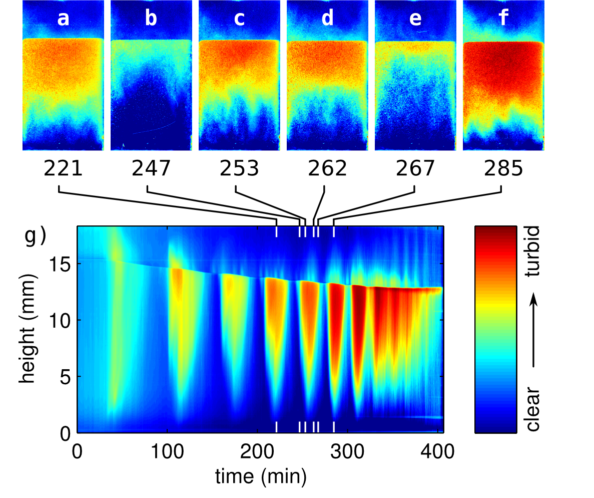
Figure 1: Episodic precipitation in binary mixtures. Panels a–f show false-colour plots of the turbidity distribution in snap shots of the phase separation of an isobutoxyethanol/water mixture subjected to a ramp rate, $\xi=2.5\times 10^{-5}\,$s^-1. Averaging in horizontal direction and arranging the resulting vertical turbidity profiles next to each other produces a space-time plot of the time evolution of the turbidity, panel g. The length scale is provided on its ordinate axis, and the scales in the pictures a)–f) can be inferred by noticing that panel g shows the full height of the samples. In section 2 we provide full details on the experimental setup and method, and in Movie 1 we supply the full evolution in the false colours presented here, together with an animation illustrating the construction of the space-time plot.

In spite of the abundance of applications, there are many unresolved issues in the quantitative description of precipitation. For instance, a better understanding of rain formation has been identified as one of the key ingredients of improved models for climate modeling (GrabowskiWang2013; BlythLowensteinHuangCuiDaviesCarslaw2013) and small-scale weather prediction (StevensSeifert2008). Here, we present a comprehensive set of experimental data that allows us to critically survey the parameter dependence of the time scale $\Delta t$ for rain formation. Data are provided for two binary fluid mixtures where demixing is driven by a continuous temperature ramp. When the ramp induces a constant generation of material, characterised by a constant value of the ramp rate, $\xi$, we observe repeated waves of aggregate nucleation, growth and precipitation (figure 1). We denote these waves of precipitation as episodic precipitation. The defining feature of episodic precipitation is an oscillatory evolution of the aggregate size distribution and of the precipitation rate in response to a slow continuous mass or heat flux into a fluid mixture. The flux leads to aggregate nucleation and growth, and episodic release of the accumulated material by precipitation events. The modulations of the precipitation rates has been observed in laboratory experiments where phase separation in a binary fluid was monitored during pressure release (SoltzbergBowersHofstetter1997) or a temperature ramp (MirzaevHeimburgKaatze2010; auernhammer05JCP; LappRohloffVollmerHof2012).

Constant driving, $\xi$, induces periodic waves of precipitation in both coexisting phases (figure 1). We identify the time scale $\Delta t$ for rain formation as the period of the episodic response in the observed demixing. Hence, we obtain comprehensive data sets for the dependence of the time scale $\Delta t$ on the viscosity, the diffusion coefficient, the mass density contrast, the number density of aggregates and the driving. The latter all vary over several orders of magnitude in our experiments (cf. appendix LABEL:sec:MatConst).

The data on $\Delta t$ is compared to a low-dimensional model that accounts for diffusive growth of small aggregates, and a crossover to collection-dominated growth for large aggregates. The model differs from classical models of rain formation by modeling the diffusive growth according to state-of-the-art models for nanoparticle synthesis (Sugimoto1992; TokuyamaEnomoto1993; Leubner2000; ClarkKumarOwenChan2011), rather than adapting classical Ostwald ripening (Houghton1959; Wilkinson2014). We will show that these assumptions are sufficient to quantitatively predict the values of $\Delta t$ for the demixing of binary fluid mixtures, and to faithfully capture the dependence of the period on their material constants, the number density of droplets and the ramp rate.

For the demixing of binary fluid mixtures the time scale, $\Delta t$, is selected by a bottleneck arising at the crossover from the diffusive growth of small aggregates to growth dominated by collection of other aggregates. The crossover emerges once the motion of the largest aggregates is affected by buoyancy. All applications mentioned above share conditions where the overall droplet volume is growing in time. Under these conditions the diffusive growth is typically dramatically faster than for classical Ostwald ripening, i.e. in circumstances where the overall droplet volume is preserved and the droplet number decays like one over time. Indeed, for all experimentally accessible ramp rates, $\xi>0$, droplet growth progresses at a constant aggregate number density (Sugimoto1992; Leubner2000; TokuyamaEnomoto1993; ClarkKumarOwenChan2011; VollmerPapkeRohloff2014). The focus of the present paper will therefore be the characterisation and modeling of aggregate growth and precipitation in settings with a sustained constant growth speed $\xi$ of the overall aggregate volume fraction, and the analysis of the dependence of $\Delta t$ on $\xi$, the aggregate concentration $n$, and appropriate material constants.

The paper is organised as follows: In section 2 we provide details on the considered mixtures, and the experimental procedure to determine $\Delta t$. It culminates in the presentation of a large data set that clearly establishes a strong dependence of $\Delta t$ on the ramp rate $\xi$. The robust features of episodic precipitation call for a universal description of the oscillation period. Such a theory is established in section 3. The resulting prediction is in very good quantitative agreement with the experimental data. (All material constants needed for the quantitative comparison are provided in appendix LABEL:sec:MatConst.) The model allows us to revisit problems encountered in quantitative descriptions of warm terrestrial rain (section LABEL:sec:discussion): diffusive droplet growth in a classical Ostwald-like scenario is too slow to account for the observed time scale, $\Delta t$. In contrast, our new model provides estimates for clouds that are too fast. We attribute this to simplifications of the droplet collision kernel that are well-justified for binary mixtures with relatively small settling rates, but that substantially overestimate the growth rate in systems, like terrestrial rain, with large density contrast of the coexisting phases. We conclude in section LABEL:sec:conclusion with a summary of our main results, and a discussion of extensions of the model that will allow us to address precipitation arising in other settings.

2 Experiment

We will discuss the parameter dependence of $\Delta t$ for repeated waves of precipitation in two well-controlled laboratory experiments: mixtures of isobutoxyethanol/water and of methanol/hexane that are subjected to a range of different temperature ramps. The system is contained in a light scattering cuvette and its temperature is controlled by immersion in a water bath so that we have full control over external perturbations. In our experiment, figure 1, two partially miscible liquids form two layers with a phase which is richer in the less dense fluid floating over a layer of the high-density phase. The temperature of the mixture is varied smoothly away from the phase coalescence point, $T_{\rm c}$, and the time-dependence of the temperature is engineered so that the ramp rate, $\xi$, of the droplet volume fraction remains constant in each run of the experiment. A movie illustrating the corresponding temperature evolution together with a video of the sample is provided in movie 2. In response to the ramp both layers show an alternating variation in turbidity, figure 1.a)–f) and figure 2.c). Representing this evolution in a space-time plot, figure 1.g), illustrates a variation of turbidity with a period $\Delta t_{i}$ between the $i^{\textrm{th}}$ and $(i+1)^{\textrm{st}}$ precipitation event. The accompanying periodic alternation in the turbidity and the particle size distribution are characteristics of episodic precipitation. The effect is robust. Episodic response has been observed in the particle size distribution (LappRohloffVollmerHof2012) and in calorimetric data (vollmer97JCP1; vollmer99; auernhammer05JCP; MirzaevHeimburgKaatze2010) in a vast range of binary mixtures (vollmer97JCP1; auernhammer05JCP; MirzaevHeimburgKaatze2010; LappRohloffVollmerHof2012), including olive oil and methylated spirit (vollmer07PRL). It arises in the upper as well as in the lower layer of the mixtures.

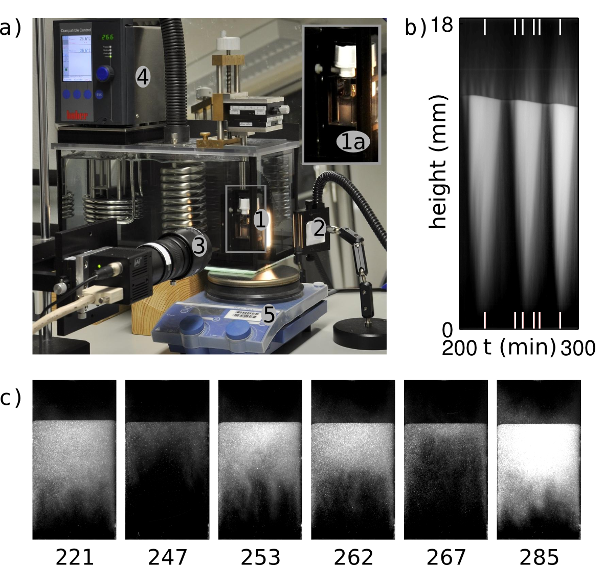
Figure 2: Setup and raw data obtained from the CCD camera. a) Photo of the experimental setup. Its components, (1)–(5) are described in the main text. b) Space-time plot based on the turbidity data provided by the camera. The sample contains a mass fraction of $0.2751$ isobutoxyethanol in water, and was subjected to a ramp rate $\xi=2.5\times 10^{-5}\,$s^-1. c) Representative snap shots of the times where the snap shots were taken are indicated below the respective photos, and by white bars in panel b). In Movie 2 we provide the full time evolution as captured by our camera.

2.1 Experimental Setup

Figure 2.a) shows the experimental setup. The sample cell (1), a $3\;$mL fluorescence cell 117.100F-QS made by Hellma GmbH, is illuminated by a KL 2500 LCD Schott cold light source (2) such that dark-field images can be taken with a BM-500CL monochrome progressive scan CCD camera (3). The camera takes $772\times 1420$ pixel images of the sample cell with a frame rate between $0.1$ and $3\;$Hz depending on the ramp rate $\xi$.

The sample temperature is controlled by immersion into a water bath that follows a temperature protocol imposed by a computer-controlled thermostat (4): an immersion cooler Haake EK20 is cooling with constant power, and a Huber CC-E immersion thermostat is heating the water bath to the preset temperature. Additionally, the temperature of the water near the sample is measured with a PT100 temperature sensor. The temperature is controlled with an accuracy of $15\,$mK. Homogenisation for repeated runs is provided by a magnetic stirring unit (5).

The inset (1a) in figure 2.a) shows a magnification of the sample cell. The camera captures the turbidity of the full cell, providing 8 bit turbidity data as shown in figure 2.c). Averaging this data in horizontal direction and plotting the resulting scans of the turbidity height profiles, provides the space-time plot figure 2.b). For visual inspection the contrast in these pictures is conveniently enhanced by a representation in false colours, figure 1. As supplementary online material we provide movies showing the black-and-white turbidity data taken by the camera together with a plot of the time evolution of the temperature, Movie 2, and an animation, Movie 1, illustrating the construction of the space-time plot of the turbidity shown in figure 1.g).

The space-time plots, figures 1.g) and 2.c), clearly visualise the period $\Delta t$ between subsequent waves of precipitation. Episodic precipitation goes along with marked oscillatory changes in the droplet size distribution (LappRohloffVollmerHof2012), and in the turbidity of the samples (auernhammer05JCP). The main panels of figure 3 show representative traces of the turbidity of the samples when heated with different, constant $\xi$. The data for $\Delta t$ are extracted from these traces as the distance between subsequent maxima of the turbidity.

In addition to capturing the turbidity we succeeded to follow the time evolution of the droplet size distribution of IBE droplets in water via an appropriately enhanced illumination and imaging (LappRohloffVollmerHof2012). Wherever available an analysis of the temporal evolution of the droplet size distributions along the same line as the one for the space-time plots of the turbidity, provides identical values for $\Delta t_{i}$ with a higher experimental accuracy. Further details on the experimental setup are provided in LappRohloffVollmerHof2012, and the data analysis used to extract the oscillation period from the space-time plots has been described in auernhammer05JCP.

2.2 Investigated Mixtures

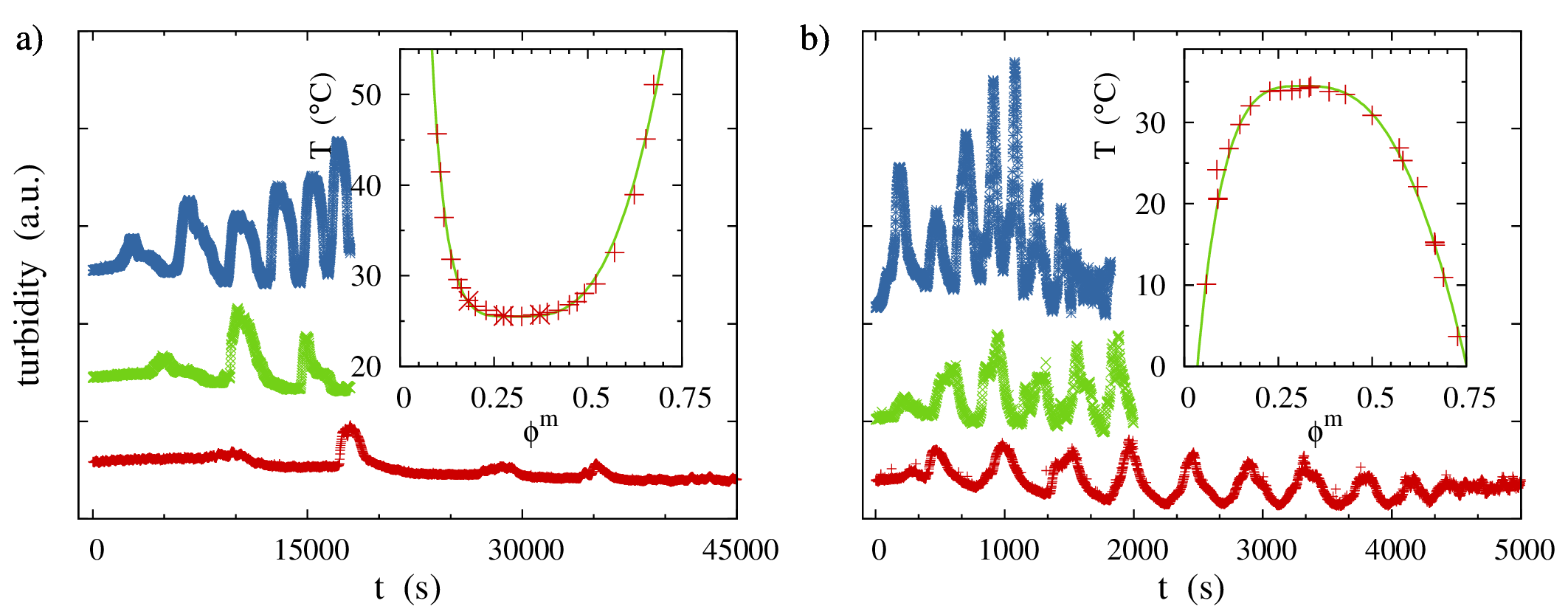
Figure 3: Phase diagrams and time traces of the turbidity. The insets show the phase diagrams of a) IBE+W, and b) M+H, and the respective main panels show oscillations of the turbidity in the lower layer for different ramp rates $\xi$: from top to bottom a) $2.5\times 10^{-5}$s^-1, $1.25\times 10^{-5}$s^-1, $5\times 10^{-6}$s^-1 for IBE+W, and b) $4\times 10^{-4}$s^-1, $2\times 10^{-4}$s^-1, $1\times 10^{-4}$s^-1 for M+H. The data points of the turbidity correspond to the average turbidity of a region of $140\,\mu$m height and the full sample width, that is located $650\,\mu$m below the meniscus. The different signals are shifted vertically for better visibility.

Two types of mixtures are considered:

Methanol/hexane (M+H)  

These mixtures are one of the classical model systems of binary phase separation (huang74; BeysensGuenounPerrot1988; AbbasSatherleyPenfold1997; IwanowskiSattarowBehrendsMirzaevKaatze2006; SamAuernhammerVollmer2011). The two liquids are fully miscible above the critical temperature $T_{\rm c}=34.45^{\circ}{\rm C}$. The concentrations of the coexisting phases that are formed for lower temperatures are shown in the phase diagram in figure 3.b). See AbbasSatherleyPenfold1997 for a detailed description.

Isobutoxyethanol/water (IBE+W)  

Mixtures of water and butoxyethanol have become popular as an experimentally-friendly system that phase separates upon heating (see e.g.  EmmanuelBerkowitz2006). For our present purposes IBE and water, figure 3.a), is even preferential since the critical point of the mixtures, $T_{\rm c}=25.61^{\circ}{\rm C}$, lies more than $10^{\circ}{\rm C}$ below the one of the butoxyethanol mixture. This further enhances the range of experimentally accessible temperatures (that must always lie well below the boiling point of water). See NakataDobashiKuwaharaKaneko1982 and LappRohloffVollmerHof2012 for more detailed descriptions.

For the fit of the coexistence curve we follow the procedure of AizpiriCorreaRubioPena1990. To first order they approximate the left and right branch of the coexistence curve by

$$\Phi_{r/l}=\Phi_{c}\pm B\>\theta^{\beta}+D\>\theta^{2\beta}$$ (1)

with the reduced temperature $\theta=|1-T/T_{c}|$, the critical point being at temperature $T_{c}$ with composition $\Phi_{c}$, and the universal scaling exponent $\beta=0.325$. For the M+H mixture this provides a good fit, the solid green line, shown in the inset of figure 3.b), with fit parameters listed in Table 1. On the other hand for IBE+W the exponent $\beta=0.325$ only applies for $\theta<10^{-3}$ (NakataDobashiKuwaharaKaneko1982), which is too small for our purposes. Even correction terms based on the Wegner expansion do not help (NakataDobashiKuwaharaKaneko1982). To have a simple set of parameters we therefore choose $\beta=0.25$, which admits a faithful description based on three free non trivial parameters (see figure 3.a) and Table 1).

	IBE	+	W	M	+	H
$\beta$	$0.25$			$0.325$
$T_{c}$ [K]	$298.76$	$\pm$	$0.12$	$307.88$	$\pm$	$0.15$
$\Phi_{c}$	$0.3093$	$\pm$	$0.0032$	$0.3143$	$\pm$	$0.0008$
$B$	$0.547$	$\pm$	$0.002$	$0.726$	$\pm$	$0.002$
$D$	$0.26$	$\pm$	$0.015$	$0.323$	$\pm$	$0.005$

Table 1: Fit parameters of the coexistence curve for IBE+W and M+H.

The temperature ramps in our experiments amount to increasing temperature for IBE+W, and decreasing temperature for M+H. For simplicity we denote this as heating, and understand that the temperature ramp rate is negative for the latter mixture. On the other hand, the ramp rate of the droplet volume fraction, $\xi$, is positive in either case, as elaborated in section 2.3.

The evolution can most conveniently be described by focusing on a region in one of the macroscopic phases. Its average concentration changes due to sedimentation of large droplets. However, immediately after a precipitation event, the bulk and the remaining small droplets are very close to an equilibrium composition at points on the coexistence curve with composition $\Phi_{b}$ for the bulk phase, and $\Phi_{d}$ for the remaining droplets in the fluid. The phases occupy the volumes $V_{b}$ and $V_{d}$, respectively.

As the mixture is further heated, the equilibrium concentrations of the coexisting phases change in response to the broadening of the miscibility gap, i.e. the region bounded by the coexistence curve. A temperature difference $\delta T$ causes a change in the equilibrium composition by $\delta\Phi_{b}<0$ and $\delta\Phi_{d}>0$. It gives rise to a concentration current across the interface of the droplets, which in turn leads to a growth of the droplets. In the following subsection we review how the temperature protocol of the experiments was chosen in order to fix the ramp rate, $\xi$, of the droplet volume fraction.

2.3 Calculating the ramp rate $\xi$

The derivation of the ramp rate, $\xi$, starts from the the average composition

$$\phi=v_{d}\Phi_{d}+(1-v_{d})\>\Phi_{b}$$ (2)

of a small volume of a mixture, where droplets of composition $\Phi_{d}$ occupy a volume fraction $v_{d}$ in a background phase of composition $\Phi_{b}$. By definition, the average composition, $\phi$, is preserved when the droplets start growing in response to a change of temperature. On the other hand droplet growth is accompanied by a change of the composition of the phases,

$$0=\dot{\phi}=v_{d}\,\dot{\Phi}_{d}+\Phi_{d}\,\dot{v}_{d}+(1-v_{d})\,\dot{\Phi}_{b}-\Phi_{b}\,\dot{v}_{d}\,.$$ (3)

We introduce the notations

$$\zeta = \Phi_{0}^{-1}\;\frac{\mathrm{d}\bar{\Phi}}{\mathrm{d}t}$$ (4a)

$$\xi = \Phi_{0}^{-1}\;\frac{\mathrm{d}\Phi_{0}}{\mathrm{d}t}$$ (4b)

$$\varphi = \frac{\phi-\bar{\Phi}}{\Phi_{0}}$$ (4c)

$$\textrm{where}\qquad\bar{\Phi} = \frac{1}{2}\;\left(\Phi_{b}+\Phi_{d}\right)\,,$$ (4d)

$$\Phi_{0} = \frac{1}{2}\;\left(\Phi_{b}-\Phi_{d}\right)\,,$$ (4e)

and substitute the resulting expressions for $\dot{\Phi}_{d}$ and $\dot{\Phi}_{b}$ into (3). Solving for $\dot{v}_{d}$ one obtains then after some straightforward algebra

$$\dot{v}_{d}=\frac{1}{2}\left(\zeta+\xi\varphi\right)\,.$$ (5)

Here, $\varphi$ is the reduced average concentration defined in (4c). It takes the value $\varphi=1$ when $\phi=\Phi_{b}$, and smaller values for compositions inside the miscibility gap.

Assuming local equilibrium one can characterise the local bulk concentration by the space dependent field $\varphi(x,t)$. Its time evolution obeys a diffusion equation with a source strength of $2\,\dot{v}_{d}$ (cates03PhilTrans). According to the above consideration this source term gives rise to a corresponding growth of the equilibrium droplet volume fraction. From the point of view of the transport equations, the magnitude of the source strength $\dot{v}_{d}$ appears therefore as the relevant parameter characterising how strongly the mixture is driven away from equilibrium. With this motivation we consider here temperature protocols that correspond to fixed values of $\dot{v}_{d}$.

In (4) it is understood that $\Phi_{0}$ and $\bar{\Phi}$ are functions of $T(t)$ due to their dependence of $\Phi_{d}$ and $\Phi_{b}$, i.e. on the borders of the two-phase region of the phase diagram. In general these functions have a different temperature dependence. Hence, it is not clear a priory that $\dot{v}_{d}$ can be fixed to a constant value by choosing an appropriate form of the temperature ramp $T(t)$. Indeed, we choose different temperature protocols for the two phases—i.e. for the M+H (and IBE+W) mixtures we adopt different temperature ramps for methanol (IBE) droplets in hexane (water) than for hexane (water) droplets in methanol (IBE). The optimal protocol is found by rearranging (5) to take the form

$$\dot{v}_{d}=\frac{1}{2\Phi_{0}(T)}\frac{\mathrm{d}\Phi_{b}}{\mathrm{d}t}-\frac{v_{d}}{\Phi_{0}}\;\frac{\mathrm{d}\Phi_{0}}{\mathrm{d}t}\approx\frac{1}{2\Phi_{0}(T)}\frac{\mathrm{d}\Phi_{b}}{\mathrm{d}T}\frac{\mathrm{d}T}{\mathrm{d}t}\,,$$ (6)

where the approximation in the final step is based on the fact that the volume fraction of droplets $v_{d}$ is always small in our experiments. According to (6) the ramp rate $\dot{v}_{d}$ for droplets in the upper and lower layer of our samples is found by appropriately assigning the indices $b$ and $d$ to the respective branches of the phase diagram. Subsequently, the temperature protocol of the ramp is obtained by integrating

$$\frac{\mathrm{d}T}{\mathrm{d}t}=2\,\dot{v}_{d}\;\Phi_{0}(T)\;\left(\frac{\mathrm{d}\Phi_{d}}{\mathrm{d}T}\right)^{-1}\,.$$ (7)

In practice there is only a small difference between $\dot{v}_{d}$ and $\xi$ since $\zeta\ll\xi$ for the phase diagrams under consideration, and since $\varphi$ is always very close to one. Hence, on the one hand, we distinguish between $\dot{v}_{d}$ and $\xi$ for the sake of calculating the temperature protocol. This avoids systematic errors in the numerical integration of (7). On the other hand, for the further presentation of the data, we specify the ramp rate in terms of $\xi$. This allows us to use terminology that is consistent with the pertinent literature (cates03PhilTrans; vollmer99; auernhammer05JCP; vollmer07PRL; LappRohloffVollmerHof2012).

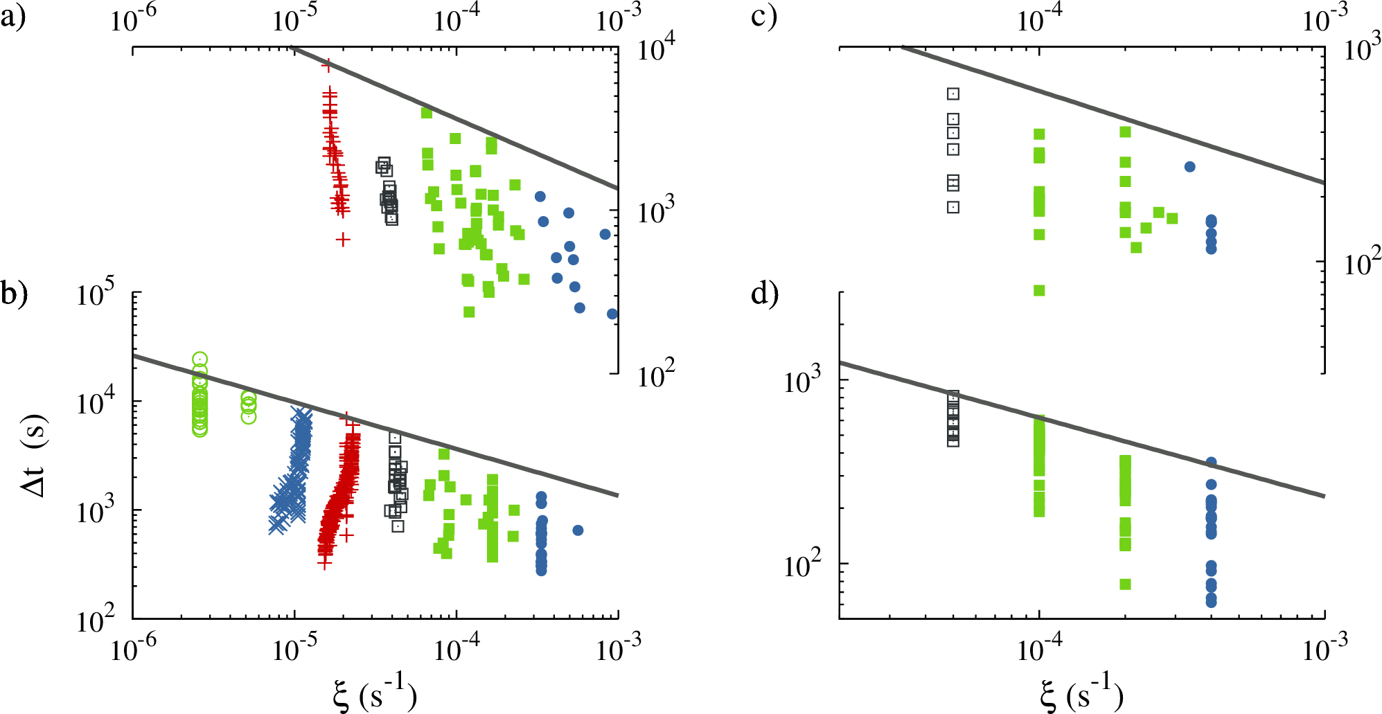
Figure 4: The oscillation period, $\Delta t$, plotted vs. the ramp rate $\xi$. The four panels show $\Delta t$ for a) water-rich droplets in an IBE-rich continuous phase, b) IBE-rich droplets in a water-rich continuous phase, c) methanol-rich droplets in a hexane-rich continuous phase, and d) hexane-rich droplets in a methanol-rich continuous phase, respectively. The different symbols denote measurements for different ranges of ramp rates, $\xi$. The colours and symbols encode different heating rates $\xi$: open green circle, $\xi<6\times 10^{-6}\,$s^-1; blue cross, $10^{-6}\,$s${}^{-1}<\xi<1.3\times 10^{-5}\,$s^-1; red plus, $1.3\times 10^{-5}\,$s${}^{-1}<\xi<3\times 10^{-5}\,$s^-1; open black square, $3\times 10^{-5}\,$s${}^{-1}<\xi<6\times 10^{-5}\,$s^-1; green square, $6\times 10^{-5}\,$s${}^{-1}<\xi<3\times 10^{-4}\,$s^-1; and blue circle, $3\times 10^{-4}\,$s${}^{-1}<\xi$. The grey lines are guides to the eye that indicate the slope of a power law, $\Delta t\sim\xi^{-3/7}$.

2.4 Experimental results for $\Delta t$

Figure 4 compiles data of $\Delta t$ for a vast range of heating rates $\xi$, and four different scenarios of phase separation in a binary mixture: a) the emergence and sedimentation of water-rich droplets in an isobutoxyethanol-rich phase; b) the emergence and rising of isobutoxyethanol-rich droplets in a water-rich phase; c) the emergence and sedimentation of methanol-rich droplets in a hexane-rich phase; and d) the emergence and rising of hexane-rich droplets in a methanol-rich phase.

Different data points for a given ramp rate are due to the drift of $\Delta t$ when pertinent material constants change upon moving further away from the critical point. In appendix LABEL:sec:MatConst we provide the temperature dependence of the material constants, which in turn translates to a time dependence when inverting the protocol $T(t)$ of the temperature ramp. For all data the height of the layer was $h\approx 1\,{\rm cm}$. Measurements for samples with varying heights between $h=0.25\,{\rm cm}$ and $5.5\,{\rm cm}$ for the lower layer showed that $\Delta t$ is hardly affected by $h$. The data points for the IBE+W mixture (left) are obtained by particle tracking (cf. LappRohloffVollmerHof2012 for experimental details), and those for M+H (right) refer to subsequent minima of turbidity measurements as shown in figure 3. We verified that both methods provide the same results. However, the data obtained from droplet tracking tend to be more accurate.

In the following section we establish a model for the droplet growth and sedimentation that provides a quantitative description of $\Delta t$ for all data presented in figure 4.

3 Theory

As a first step to model $\Delta t$ we consider the reasons why the turbidity — and hence the precipitation rate — in our experiment is not steady: the turbidity of a transparent fluid mixture increases when a considerable number of droplets have grown to a size comparable to (and eventually larger than) the wavelength of light. This manifests as a change of colour in the lower part of the cell when the system progresses from the snapshots shown in figure 1.b)–c). Conversely, the fluid becomes clearer again when vast amounts of small droplets are collected during the sedimentation of the largest droplets (transition from figure 1.d)–e)). Repetition of the cycle of nucleation, growth of droplets, and resetting the system by sedimentation gives rise to episodic precipitation, as shown in the space-time plot, figure 1.g). In the following the salient features of this dynamics are modelled.

3.1 Evolution of the radius of the largest droplets

We start with general considerations motivating the setup of the model.

1. Spatial degrees of freedom need not be considered to describe the evolution of the largest droplets. For the nonlinear reactions terms characterising phase separation the convective mixing efficiently eliminates spatial inhomogeneities of the droplet size distribution (BenczikVollmer2010; BenczikVollmer2012). Indeed, based on visual inspection of the accompanying movies, we estimate the mixing time scale to be of the order of seconds. It is about three orders of magnitude smaller than the period $\Delta t$.

2. It is sufficient to consider the characteristic size of the largest droplets rather than the full droplet size distribution. For diffusively growing droplets the size distribution is sharply bounded towards large droplets. Consequently, the largest droplets in the system have a well-defined size and there are only few of these droplets (Slezov2009; ClarkKumarOwenChan2011; VollmerPapkeRohloff2014). When buoyancy starts to effect their motion these large droplets collect smaller droplets, grow rapidly, and eventually clear the system from droplets by precipitation (KostinskiShaw2005).

3. While many different processes contribute to the droplet growth, it suffices to consider only droplet growth by diffusive accretion that relaxes supersaturation, and the collection of small droplets by sedimenting large ones in order to achieve a quantitative description of $\Delta t$. The processes are illustrated in figure 5, and we will now discuss them in turn.

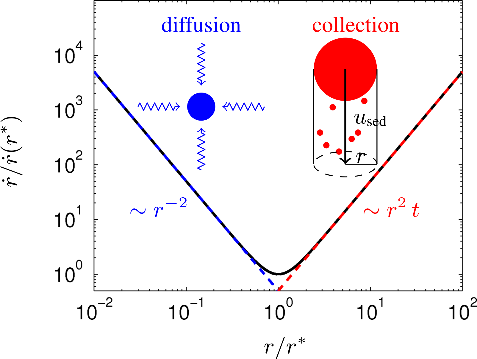
Figure 5: Bottleneck in droplet growth. As a function of droplet size $r$ the growth speed $\dot{r}$ of droplets shows a sharp minimum at a size $r^{\ast}$. Smaller droplets grow by diffusion — the growth of larger droplets is speeded up by sedimentation, that promotes the collection of small droplets (see insets).

3.1.1 Growth by diffusive accretion that relaxes supersaturation

The dynamics of large droplets crossing the meniscus (AartsDullensLekkerkerker2005) and droplet nucleation (BinderStauffer1976; FarjounNeu2011) provide microscopic droplets in the fluid. Subsequently, the supersaturation in the bulk relaxes by diffusion of the minority component onto the droplets. The diffusive accretion of material on the droplets relaxes supersaturation and induces droplet growth.

In the experiments the temperature ramp is adjusted in such a way that the volume fraction of droplets grows linearly in time with a speed $\xi$. For these growth conditions it was demonstrated in Sugimoto1992; TokuyamaEnomoto1993; ClarkKumarOwenChan2011; VollmerPapkeRohloff2014 that the number density of droplets is preserved. Droplets of a characteristic radius $r$ and number density $n$ occupy a volume fraction $n\,4\pi r^{3}/3$. When the droplet volume fraction increases with speed $\xi$ and the number density $n$ is conserved, diffusive growth provides a temporal change of the droplet radius

$$\frac{\mathrm{d}}{\mathrm{d}t}\frac{4\pi\,n\,r^{3}}{3}=\xi\quad\Rightarrow\quad\dot{r}=\frac{\xi}{4\pi n}\;\frac{1}{r^{2}}\;.$$ (8)

Alternatively, this growth law can be obtained as large $k$ approximation of the diffusive growth law (ClarkKumarOwenChan2011; VollmerPapkeRohloff2014)

$$\dot{a}=\frac{\sigma D}{a^{2}}\left(k\,\frac{a}{\langle a\rangle}-1\right)\,,\quad k=1+\frac{\xi}{4\pi\sigma Dn}$$ (9)

describing the growth of a droplet of radius $a$ in an assembly of droplets with distribution $P(a)$ and mean droplet radius $\langle a\rangle=\int\mathrm{d}a\,a\,P(a)$. In (9) $D$ is the diffusion coefficient for accretion of material on the droplets, and

$$\sigma=\frac{2\gamma V_{m}^{2}C_{\infty}}{RT}$$ (10)

is the Kelvin length (Lif+81; Bray1994), that depends on the interfacial tension $\gamma$, the molar volume $V_{m}$, and the equilibrium composition of the droplet phase $C_{\infty}$ in units of mol/m³. (Specific values of the material constants are provided in appendix LABEL:sec:MatConst.) It was shown in VollmerPapkeRohloff2014 that $k$ takes values of the order to $10^{6}$ under the conditions considered here, and that $a\simeq\langle a\rangle$ in the late stages of competitive droplet growth at large $k$. Hence, (9) reduces to (8).

3.1.2 Growth by collection of smaller droplets

When the droplets become sufficiently large, they drift under the influence of buoyancy forces. According to Stokes’ formula the velocity of a slowly settling droplet is (TaylorAcrivos1964; guyonBook)

$$u=\kappa r^{2}\qquad\textrm{with}\quad\kappa=\frac{2}{9}\;\frac{g\,\Delta\rho}{\mu_{b}}\;\frac{\mu_{d}+\mu_{b}}{\mu_{d}+\frac{2}{3}\mu_{b}}\>,$$ (11)

where $g$ is the gravitational acceleration, $\Delta\rho$ the density contrast, $\mu_{b}$ is the dynamic viscosity of the bulk phase, and $\mu_{d}$ is the viscosity of the material in the droplets. When the Stokes velocity of the the largest droplets in the system becomes noticeable they collect smaller droplets in their path. Hence, the volume of a large droplet grows like $4\pi r^{2}\,\dot{r}=\varepsilon\pi r^{2}u\xi t$, where $\varepsilon$ is the collection efficiency for large droplets coalescing with smaller ones, and $\xi t$ is the volume fraction of the smaller droplets. (Observe that $r$ refers to the radius of the largest droplets in the system—a minute minority of droplets that accounts for only a small part of the droplet volume fraction.) Accordingly, we find the collisional growth rate

$$\dot{r}=\frac{\varepsilon\kappa\xi t}{4}r^{2}\;.$$ (12)

3.1.3 The bottleneck of droplet growth

The diffusive growth mechanism, (8), works very well for small droplets due to the factor $r^{-2}$, and it becomes less and less efficient when $r$ grows. In contrast, growth by collecting small droplets, (12), does not contribute to the growth as long as all droplets are small, while it leads to runaway growth of the large droplets when their motion is affected by buoyancy. Hence, we assert that the sum of the diffusive growth, (8), and the contribution accounting for the collection of smaller droplets, (12),

$$\dot{r}=\frac{\xi}{4\pi n}\frac{1}{r^{2}}+\frac{\varepsilon\kappa\xi t}{4}r^{2}\,,$$ (13)

faithfully describes the growth of the largest droplets in the system. The growth law, (13), shows a bottleneck of growth at the bottleneck radius, $r^{\ast}$, where the droplet growth speed, $\dot{r}$, takes its smallest value, $\dot{r}(r^{\ast},t^{\ast})=(2/3)\left(r^{\ast}\right)^{-2}$ (see figure 5),